Estimation of a Structural Vector Autoregression Model
Using Non-Gaussianity
Aapo Hyv¨arinen [email protected]
Department of Mathematics and Statistics∗ University of Helsinki
Helsinki, Finland
Kun Zhang [email protected]
Department of Computer Science and HIIT University of Helsinki
Helsinki, Finland
Shohei Shimizu [email protected]
Institute of Scientific and Industrial Research Osaka University
Osaka, Japan
Patrik O. Hoyer [email protected]
Department of Computer Science and HIIT University of Helsinki
Helsinki, Finland
Editor: Peter Dayan
Abstract
Analysis of causal effects between continuous-valued variables typically uses either autoregressive models or structural equation models with instantaneous effects. Estimation of Gaussian, linear structural equation models poses serious identifiability problems, which is why it was recently pro-posed to use non-Gaussian models. Here, we show how to combine the non-Gaussian instantaneous model with autoregressive models. This is effectively what is called a structural vector autoregres-sion (SVAR) model, and thus our work contributes to the long-standing problem of how to estimate SVAR’s. We show that such a non-Gaussian model is identifiable without prior knowledge of net-work structure. We propose computationally efficient methods for estimating the model, as well as methods to assess the significance of the causal influences. The model is successfully applied on financial and brain imaging data.
Keywords: structural vector autoregression, structural equation models, independent component
analysis, non-Gaussianity, causality
1. Introduction
Analysis of causal influences or effects has become an important topic in statistics and machine learning, and has recently found applications in, for example, neuroinformatics (Roebroeck et al., 2005; Kim et al., 2007) and bioinformatics (Opgen-Rhein and Strimmer, 2007). While the deeper meaning of causality has been formalized in different ways (Pearl, 2000; Spirtes et al., 1993), we
consider the problem here from a practical viewpoint, where coefficients in conventional statistical models are interpreted as causal influences.
For continuous-valued variables, such an analysis is typically performed in two different ways. First, if the time-resolution of the measurements is higher than the time-scale of causal influences, one can estimate a classic autoregressive (AR) model with time-lagged variables and interpret the autoregressive coefficients as causal effects. Second, if the measurements have a lower time resolu-tion than the causal influences, or if the data has no temporal structure at all, one can use a model in which the influences are instantaneous, leading to Bayesian networks or structural equation models (SEM); see Bollen (1989).1
While estimation of autoregressive methods can be solved by classic regression methods, the case of instantaneous effects is much more difficult. Most methods suffer from lack of identifi-ability, because covariance information alone is not sufficient to uniquely characterize the model parameters. Prior knowledge of the structure (fixing some of the connections to zero) of the SEM is then necessary for most practical applications. However, a method was recently proposed which uses the non-Gaussian structure of the data to overcome the identifiability problem (Shimizu et al., 2006). If the disturbance variables (external influences) are non-Gaussian, no prior knowledge on the network structure is needed to estimate the linear SEM, except for the ubiquitous assumption of a directed acyclic graph (DAG) and the assumption of no latent variables. (The case of latent variables, that is, unobserved confounders, was later considered by Hoyer et al., 2008.)
Here, we consider the general case where causal influences can occur either instantaneously or with considerable time lags. Such models are one example of structural vector autoregressive (SVAR) models popular in econometric theory, in which numerous attempts have been made for its estimation, see, for example, Swanson and Granger (1997), Demiralp and Hoover (2003) and Moneta and Spirtes (2006). We propose to use non-Gaussianity to estimate the model. We show that this variant of the model is identifiable without other restrictions on the network structure than acyclicity and no latent variables. To our knowledge, no model proposed for this problem has been shown to be fully identifiable without prior knowledge of network structure. We further propose two computationally efficient methods for estimating the model based on the theory of independent component analysis or ICA (Hyv¨arinen et al., 2001).
The proposed non-Gaussian model not only allows estimation of both instantaneous and lagged effects; it also shows that taking instantaneous influences into account can change the values of the time-lagged coefficients quite drastically. Thus, we see that neglecting instantaneous influences can lead to misleading interpretations of causal effects. The framework further points towards general-izations of the well-known Granger causality measure (Granger, 1969).
The paper is structured as follows. We first define the model and discuss its relation to other models in Section 2. We motivate the key assumption of non-Gaussianity in Section 3. Next, we de-rive the likelihood and discuss some of its interpretations in Section 4. In Section 5 we propose two computationally efficient estimation methods and compare them with simulations. Assessement of the results using testing is considered in Section 6. Section 7 discusses some interesting phenomena concerning the interpretation of the estimated parameter values. Experiments on financial and neu-roscientific data are made in Section 8. Some extensions of the model are discussed in Section 9, and Section 10 concludes the paper. Preliminary results were published in Hyv¨arinen et al. (2008) and Zhang and Hyv¨arinen (2009).
2. A Non-Gaussian Structural Vector Autoregressive Model
In this section, we define our new model.
2.1 Background and Notation
Let us denote the observed time series by xi(t),i=1, . . . ,n,t=1, . . . ,T where i is the index of the
time series and t is the time index. All the time series (variables) are collected into a single column vector x(t). Without loss of generality, we can assume that the xi(t)have zero mean.
In autoregressive modelling, we would model the dynamics by a model of the form
x(t) =
k
∑
τ=1Bτx(t−τ) +e(t) (1)
where k is the number of time-delays used, that is, the order of the autoregressive model, Bτ,τ= 1, . . . ,k are n×n matrices, and e(t)is the innovation process.
In structural equation models (SEM), or continuous-valued Bayesian networks, there is no time structure in the data, and the variables are simply modelled as functions of the other variables:
x=Bx+e (2)
where the vector e is the vector of disturbances or external influences. The diagonal of B is defined to be zero. It is typically assumed that we have a sample of observations which are independent and identically distributed.
2.2 Definition of Our Model
In many applications, the influences between the xi(t)can be both instantaneous and lagged. Thus,
we combine the two models in (1) and (2) into a single model. Denote by Bτ the n×n matrix of the causal effects between the variables xi with time lagτ,τ=0, . . . ,k . Forτ>0, the effects
are ordinary autoregressive effects from the past to the present, while for τ=0, the effects are “instantaneous”.
We define our model by a straightforward combination of (1) and (2) as
x(t) =
k
∑
τ=0Bτx(t−τ) +e(t) (3)
where the ei(t)are random processes modelling the disturbances. We make the following
assump-tions on the ei(t):
1. The ei(t)are are mutually independent, both of each other and over time. This is a typical
assumption in autoregressive models.
2. The ei(t)are non-Gaussian, which is an important assumption which distinguishes our model
from classic models, whether autoregressive models, structural-equation models, or Bayesian networks.
in Section 9. The acyclicity is equivalent to the existence of a permutation matrix P, which corresponds to a “causal” ordering of the variables xi, such that the matrix PB0PT is lower-triangular (i.e., entries above the diagonal are zero). Acyclicity also implies that the entries on the diagonal are zero, even before such a permutation.
2.3 Relation to Other Models
Next, we discuss the relationships of our model with other models.
2.3.1 LINEARNON-GAUSSIANACYCLICMODEL
Our model is a generalization of the linear non-Gaussian acyclic model (LiNGAM) proposed in Shimizu et al. (2006). If the order of the autoregressive part is zero, that is, k=0, the model is nothing else than the LiNGAM model, modelling instantaneous effects only. As shown in Shimizu et al. (2006), the assumption of non-Gaussianity of the eienables estimation of the model. This is
because the non-Gaussian structure of the data provides information not contained in the covariance matrix which is the only source of information in most methods.
Non-Gaussianity enables model estimation using independent component analysis, which solves the non-identifiability of factor analytic models using the assumption of non-Gaussianity of the fac-tors (Comon, 1994; Hyv¨arinen et al., 2001). In fact, the estimation method in Shimizu et al. (2006) uses an ICA algorithm as an essential part. This is because we can transform (2) into the factor-analytic model of ICA:
x= (I−B)−1e (4)
where e is now a vector of latent variables. Under the assumptions of the model, in particular the independence and non-Gaussianity of the disturbances ei, the model can be essentially estimated
(Comon, 1994). The acyclicity assumption also ensures that I−B is invertible.
However, there is an important indeterminacy which ICA cannot solve: the order of the compo-nents. In a SEM, each disturbance corresponds to one of the observed variables. In contrast, ICA, like most factor-analytic models, gives the factors in no particular order. Thus, after ICA estimation (or as part of the ICA estimation) we have to establish the correspondence between the xiand the ei.
It was proven by Shimizu et al. (2006) that the correspondence can in fact be established based on the acyclicity of B. Basically, only one of the possible orderings of the rows of(I−B)is such that all the elements on the diagonal are non-zero, and can thus be scaled to equal one, which has to be the case by definition.
Thus, the LiNGAM model can be estimated by basically first performing ICA estimation and then finding the right ordering of the components based on acyclicity.
2.3.2 AUTOREGRESSIVEMODELS
On the other hand, if the matrix B0 has all zero entries, the model in Eq. (3) is a classic vector autoregressive model in which future observations are linearly predicted from preceding ones. If we knew in advance that B0is zero, the model could thus be estimated by classic regression techniques since we do not have the same variables on the left and right-hand sides of Eq. (3). However, our model would still be different from classic autoregressive models because the disturbances ei(t)are
It is important to note here that an autoregressive model can serve two different goals: prediction and analysis of causality. Our goal here is the latter: We estimate the parameter matrices Bτin order to interpret them as causal effects between the variables. This goal is distinct from simply predicting future outcomes when passively observing the time series, as has been extensively discussed in the literature on causality (Pearl, 2000; Spirtes et al., 1993). Thus, we emphasize that our model is not intended to reduce prediction errors if we want to predict xi(t)using (passively) observed values of
the past x(t−1),x(t−2), . . .; for such prediction, an ordinary autoregressive model is likely to be just as good.
2.3.3 STRUCTURAL VECTORAUTOREGRESSIVEMODELS
Combinations of SEM and vector autoregressive models have been proposed in the econometric literature, and called structural vector autoregressive models (SVAR). Although many of them are quite similar to our model in spirit (Swanson and Granger, 1997; Demiralp and Hoover, 2003; Moneta and Spirtes, 2006), we are not aware of any method in which non-Gaussianity would be an essential assumption. We will see below how the assumption of non-Gaussianity is essential for the identifiability of the model, which has been a serious problem in previous methods. In the next section, we thus consider the justification of this assumption.
3. Why Disturbances Could be Non-Gaussian
Non-Gaussianity is the new assumption in our model. In this section, we attempt to justify why, in many applications, we can consider the ei(t) to be non-Gaussian. The arguments are based on
heteroscedasticity. We do not by any means claim that we are the first to develop these arguments; some of them are well-known and we merely re-iterate them here.
The principle of heteroscedasticity means that the variance of ei(t)depends on t: in some parts
of the time series, it is larger, and in other parts it is smaller. The shape of the distribution conditional to the variance is the same always: often it is assumed to be Gaussian (normal).
We argue that heteroscedasticity is an important reason why, in many cases, the ei(t)should be
strongly non-Gaussian. Even if the Central Limit Theorem is applicable in the sense that ei(t)is a
sum of many different latent independent variables, the disturbances can be very non-Gaussian if, for some reason, the variance of the ei(t)is changing.
The connection between heteroscedasticity and non-Gaussianity can be developed in a few sim-ple equations. Denote by z(t)a standardized Gaussian random variable. Assume that a disturbance e(t)(dropping the index i for simplicity) is a product of z and a random “variance” variable v(t):
e(t) =z(t)v(t)
We can simply show the following well-known result: If z is Gaussian, e has always positive kurtosis,2regardless of the distribution of v (as long as v2has non-zero variance). This is because
kurt(e) =E{e4} −3(E{e2})2=E{v4z4} −3(E{v2z2})2=3[E{v4} −(E{v2})2] (5) which is always positive because it is the variance of v2multiplied by three (Beale and Mallows, 1959). It is easy to generalize this result to show that even if z is not Gaussian, the kurtosis is still positive if the variance of v2is large enough.
Heteroscedastity can be seen in some important application areas of causal modelling, in partic-ular:
1. In econometrics, heteroscedastic models have a long tradition (Engle, 1995). For example, in financial markets the volatility of a price is often assumed to be changing over time, and volatility is nothing but the variance in some scaling.
2. In brain imaging, the power of rhytmic activity as measured by electroencephalography or magnetoencephalography is non-constant (Hari and Salmelin, 1997). The power is essentially the same as the variance.
We emphasize that the assumption of non-Gaussianity is fundamentally an empirical assump-tion. It is fulfilled in some application areas and not in others. It can be validated by examining the distributions of the estimates of the ei(t), which are simply obtained by solving for e(t)in (3)
after estimation of the model. Those estimates are linear functions of the data, which implies that if the data were Gaussian, the ei(t)would necessarily be Gaussian. Thus, any non-Gaussianity in
the estimates is valid evidence for the Gaussianity of the underlying ei(t). In addition to visual
inspection, any formal tests for non-Gaussianity can be used, such as the Shapiro-Wilk test or the Kolmogorov-Smirnov test. (Independence of the ei(t)can be validated in the same way, although it
seems to be more difficult to investigate by visualization or testing.)
However, in practice the question is not whether the disturbances are non-Gaussian but whether they are sufficiently far from Gaussian to enable sufficiently accurate estimation. In the theory of ICA, it has been shown that the asymptotic variance of the estimators is a function of the non-Gaussianity of the components: When their distribution approaches non-Gaussianity, the asymptotic variance goes to infinity (Cardoso and Laheld, 1996; Hyv¨arinen et al., 2001). Thus, instead of testing non-Gaussianity it may be much more useful to simply measure the accuracy of the estimates by bootstrapping and similar methods. If the disturbances are Gaussian (or very close to Gaussian), our estimation method is likely to fail completely. Some other assumptions are then needed to obtain identifiability of the model.
It should be also noted that the assumptions of non-Gaussianity and independence cannot be easily disentangled from the assumption of linearity. If there are non-linearities in the system, these may, for example, lead to non-Gaussian residuals even if the original disturbances were Gaussian.
4. Likelihood of the Model
To estimate our model, we start by formulating its likelihood.
4.1 Likelihood of LiNGAM
First, we derive the likelihood of the LiNGAM model (Shimizu et al., 2006) which has not yet been given in the literature. The starting point is the likelihood of the ICA model which is well-known, see, for example, Pham and Garrat (1997) and Hyv¨arinen et al. (2001). Denote the ICA model by
x=As
for a square invertible matrix A, and independent non-Gaussian latent variables si. Denote the
observed sample by X= (x(1), . . . ,x(T))and W=A−1. The log-likelihood is then usually given in the form
log L0(X) =
∑
t
∑
ilog pi(wTix(t)) +T log det|W|
where the pi are the density functions of the independent components (here: disturbances). Since
the densities of the disturbances are not specified, we have in general a semi-parametric problem. Different methods have been developed for approximating log pi, for example, Pham and Garrat
(1997), Karvanen and Koivunen (2002) and Chen and Bickel (2006). Here, we have to take into account the fact that those methods usually assume that the independent components have been normalized to unit variance, which is not the case in LiNGAM. Thus, we prefer to modify the formula by normalizing the densities as follows:
log L1(X) =
∑
t
∑
ilog ˜pi(
wTi x(t)
σi
)−T
∑
i
logσi+T log det|W| (6)
where the ˜piare the densities of the disturbances standardized to unit variance, and theσ2i are their
variances before standardization.
In fact, in practice it has been realized that often one can just fix the ˜pi to a single function and
still obtain a satisfactory estimator. In particular, if we know that the disturbances are all super-Gaussian (i.e., have positive kurtosis), fixing
log ˜pi(s) =−
√
2|s|+const.
is enough to provide a consistent estimator under weak constraints (Cardoso and Laheld, 1996; Hyv¨arinen and Oja, 1998).
In LiNGAM, we have from (4) that in terms of the ICA model, A−1=W=I−B0 (we use the subindex 0 for B in LiNGAM to comply with the notation below). Now, we can simplify the likelihood because of the DAG structure. The DAG structure means that for the right permutation of its rows (corresponding to the causal ordering), W is lower-triangular. The determinant of a triangular matrix is equal to the product of its diagonal elements, and a permutation does not change the determinant, so the determinant of W is equal to the product of the diagonal elements when the variables are ordered in the causal order. But by definition of W in LiNGAM, those diagonal elements are all equal to one, so the last term in (6) is zero. So, the likelihood of the LiNGAM model is finally given by
log L(X) =
∑
t
∑
ilog ˜pi
wTi x(t)
σi
−T
∑
i
logσi
=
∑
t
∑
ilog ˜pi
xi(t)−bT0,ix(t) σi
!
−T
∑
i
where the variances of the components can be estimated by taking the empirical variances as
σ2
i =
1
T
∑
t (xi(t)−bT
0,ix(t))2.
(Alternatively, theσicould be obtained by a separate maximization of the likelihood, but this would
be more complicated computationally and conceptually.) Here, W is constrained to correspond to a DAG, with ones added in the diagonal.
4.2 Likelihood of Our Model
Now we can derive the likelihood of our model. First note that from (3) we can derive
x(t) =
k
∑
τ=0Bτx(t−τ) +e(t)⇔ (I−B0)[x(t)−
k
∑
τ=1(I−B0)−1Bτx(t−τ)] =e(t), which gives
x(t)−
k
∑
τ=1(I−B0)−1Bτx(t−τ) =B0[x(t)−
k
∑
τ=1(I−B0)−1Bτx(t−τ)] +e(t)
which shows that the our model in (3) is a LiNGAM model for the residuals x(t)−∑kτ=1(I− B0)−1Bτx(t−τ). Denoting
Mτ= (I−B0)−1Bτ and W=I−B0 (8)
and replacing x(t)in (7) by the residuals, we have
log L(X) =
∑
t
∑
ilog ˜pi
wTi [x(t)−∑k
τ=1Mτx(t−τ)]
σi
−logσi (9)
with
σ2
i =
1
T
∑
t wT i [x(t)−
k
∑
τ=1Mτx(t−τ)]
!2 .
4.3 Information-Theoretic Interpretation
An interesting point to note is that the likelihood is now a sum of the negative entropies of the residuals. The differential entropy of a random variable s can be written using the standardized version of s, denoted by ˜s, as follows:
H(s) =−
Z
ps(u)log ps(u)du=− Z
ps˜(u)log ps˜(u)du+logσs
whereσ2
sis the variance of s. Thus, we can interpret the terms in (9) as the (negative) entropies of the
5. Practical Estimation Methods
Next we propose two practical methods for estimating the model, and further show how to include a sparseness penalty which may be very useful in practice.
5.1 A Two-Stage Method with Least-Squares Estimation
Optimization of the likelihood is difficult because it contains a complicated combinatorial opti-mization part due to the constraint that B0is acyclic. A conceptually simple way of reinforcing this constraint would be to go through all possible orderings of the observed variables, and for each of them, maximize the likelihood as a function of the Bτso that B0is constrained to be lower triangu-lar. This is obviously computationally very expensive since the number of ordering is equal to n! where n is the number of variables. Only for a very small n can this be computationally feasible. (Another difficulty is that the likelihood contains a semiparametric part because we do not specify a parametric model of the non-Gaussian distributions, but this problem has already been extensively treated in the theory of ICA, and has been found not to be very serious in practice, see Hyv¨arinen et al., 2001.)
To avoid the computational problems with likelihood, we propose a computationally simpler two-stage method for estimating our model. The method combines classic least-squares estimation of an autoregressive (AR) model with LiNGAM estimation.
5.1.1 DEFINITION
The basic idea is that the Mτ in (8) can be consistently, and computationally efficiently, estimated by classic least-squares methods. Then, since the model is essentially a LiNGAM model for the residuals of the predictions by the Mτ, we simply use our previously developed estimation methods for LiNGAM to estimate the rest of the parameters. These methods (Shimizu et al., 2006) seem to tackle the combinatorial optimization problem in a satisfactory way. The ensuing method will be justified in more detail below; it is defined as follows:
1. Estimate a classic autoregressive model for the data
x(t) =
k
∑
τ=1Mτx(t−τ) +n(t) (10)
using any conventional implementation of a least-squares method. Note that hereτ>0, so it is really a classic AR model. Denote the least-squares estimates of the autoregressive matrices by ˆMτ.
2. Compute the residuals, that is, estimates of n(t)
ˆn(t) =x(t)−
k
∑
τ=1ˆ
Mτx(t−τ).
3. Perform the LiNGAM analysis (Shimizu et al., 2006) on the residuals. This gives the estimate of the matrix B0as the solution of the instantaneous causal model
4. Finally, compute the estimates of the causal effect matrices Bτforτ>0 as
ˆ
Bτ= (I−Bˆ0)Mˆτforτ>0. (11) 5.1.2 CONSISTENCYPROOF
We now prove that this provides a consistent estimator of Bτ. First, the basic model definition in (3) can be manipulated to yield
(I−B0)x(t) =
k
∑
τ=1Bτx(t−τ) +e(t)
and thus
x(t) =
k
∑
τ=1(I−B0)−1Bτx(t−τ) + (I−B0)−1e(t). (12) Now, a well-known result is that least-squares estimation of an AR model as in (10) is consistent even if the innovation vector n(t) does not have independent or even uncorrelated elements (for fixed t), and even if it is heteroscedastic and non-Gaussian. Thus, comparing (12) with (10), in the limit we can equate the autoregressive matrices, which gives(I−B0)−1Bτ=Mτforτ≥1, and thus (11) is justified. (In fact, we anticipated (11) in the notation used in the likelihood in (9).)
Second, comparison of (12) with (10) shows that the residuals ˆn(t)are, asymptotically, of the form(I−B0)−1e(t). This means
ˆn(t) = (I − B0)−1e(t) ⇔ (I − B0)ˆn(t) = e(t) ⇔ ˆn(t) = B0ˆn(t) + e(t) which is the LiNGAM model for ˆn(t). This shows that B0is obtained as the LiNGAM analysis of the residuals, and the consistency of our estimator of B0follows from the consistency of LiNGAM estimation (Shimizu et al., 2006). Thus, our method is consistent for all the Bτ. This obviously proves, by construction, the identifiability of the model as well.
5.1.3 INTERPRETATIONRELATED TO ICAOFRESIDUALS
An interesting viewpoint of the two-stage estimation method is analysis of the dependencies of the innovations after estimating a classic AR model. Suppose we just estimate an AR model as in (1), and interpret the coefficients as causal effects. Such an interpretation more or less presupposes that the innovations ei(t)are independent of each other, because otherwise there is some structure
in the model which has not been modelled by the AR model. If the innovations are not indepen-dent, the causal interpretation may not be justified. Thus, it seems necessary to further analyze the dependencies in the innovations in cases where they are strongly dependent.
5.2 Method Based on Multichannel Blind Deconvolution
While the two-stage method proposed above is computationally very efficient, it is far from being statistically optimal. The estimation of the autoregressive part takes in no way non-Gaussianity into account and is thus likely to be suboptimal. However, it is useful because it provides a good initial guess for any further iterative method.
Thus, to improve the results of the two-stage method, we further propose an estimation method based on the similarity of our model with convolutive versions of ICA which are also called multi-channel blind deconvolution (MBD). Estimation of the model Eq. (3) is, in fact, closely related to the multichannel blind deconvolution problem with causal finite impulse response (FIR) filters (Ci-chocki and Amari, 2002; Hyv¨arinen et al., 2001). MBD, as a direct extension of ICA, assumes that the observed signals are convolutive mixtures of some spatially and independently and identically distributed (i.i.d.) sources.
Using MBD methods is justified here due to the possibility or transforming an autoregressive model into a moving-average model: In Eq. (3), the observed variables xi(t)can be considered as
convolutive mixtures of the disturbances ei(t). Thus, we can find estimates of Bτ, as well as ei(t),
in Eq. (3), by using MBD methods to estimate the filter matrices Wτ
ˆe(t) =
k
∑
τ=0Wτx(t−τ). (13)
Comparing (13) with (3), we can see that the Bτ can then be recovered from the estimated Wτ; details are given below.
The basic statistical principle to estimate the MBD model is that the disturbances ei(t)should
be mutually independent for different i and different t. Under the assumption that at most one of the sources is Gaussian, by making the estimated sources spatially and temporally independent, MBD can recover the mixing system (here corresponding to ei(t) and Bτ) up to some scaling,
permutation, and time shift indeterminacies (Liu and Luo, 1998). This implies that our SVAR model is identifiable by MBD if at most one of the disturbances eiis Gaussian.
There exist several well-developed algorithms for MBD. For example, one may adopt the one based on natural gradient (Cichocki and Amari, 2002). By extending the LiNGAM analysis proce-dure (Shimizu et al., 2006), we can find the estimate of Bτin the following three steps, based on the MBD estimates of Wτ.
1. Find the permutation of rows of W0 which yields a matrixfW0 with only significantly non-zero entries on the main diagonal. The permutation can be found using similar methods (e.g., the Hungarian algorithm) as in LiNGAM (Shimizu et al., 2006). Note that here we also need to apply the same permutations to rows of Wτ(τ>0) to producefWτ.
2. Divide each row offW0andfWτ(τ>0) by the corresponding diagonal entry infW0. This gives
f
W′0andfW′τ, respectively. The final estimates of B0 and Bτ(τ>0) can then be computed as
b
B0=I−fW′0andBbτ=−fW′τ, respectively.
5.3 Sparsification of the Causal Connections
For the purposes of interpretability and generalizability, it is often useful to sparsify the causal connections, that is, to set insignificant entries of ˆBτ to zero. Analogously to the development of ICA with sparse connections (Zhang et al., 2009), we can incorporate an adaptive L1penalty into the likelihood of the MBD method to achieve fast model selection which performs such sparsification. We use a penalty-based approach because traditional model selection based on information criteria involves a combinatorial optimization problem whose complexity increases exponentially in the dimensionality of the parameter space. In the MBD problem, this is often not computationally feasible.
Thus, to make Wτ in Eq. (13) as sparse as possible, we maximize the penalized likelihood defined as
pl({Wτ}) =log L({Wτ})−λ
∑
i,j,τ
|wi,j,τ|/|wˆi,j,τ|, (14)
where L({Wτ}) is the likelihood, wi,j,τ the (i,j)th entry of Wτ, and ˆwi,j,τ a consistent estimate of wi,j,τ, such as the maximum likelihood estimate. The parameterλis the general weight of the penalty.
The idea here is that we first compute an initial estimate of the wi,j,τby a conventional method (such as maximum likelihood) and then use those estimates to compute a parameter-wise weighting in the L1penalty. The end result is that those wi,j,τ for which the initial estimates ˆwi,j,τwere small are heavily penalized, and likely to be zero in the final estimate obtained by maximization of pl.
This penalized likelihood is a special case of adaptive Lasso and therefore has the same consis-tency in variable selection (Zou, 2006). In fact, it can also be used for selecting the order k of the autoregressive model. In particular, to achieve model selection similar to the Bayesian Information Criterion (BIC), one can setλ=log T , where T is the sample size (Zhang et al., 2009).
It may be also useful to penalize groups of parameters. In particular, to see if the historical values of xi(t)causes xj(t)(i6=j), one needs to examine the combined effect of the group of
param-eters[Bˆτ]i,j,τ=1, ...,p, and therefore it makes sense to apply penalization on the parameter group.
Combining the above approach with group Lasso (Bach, 2008) leads to the following penalized likelihood:3
pl({Wτ}) =log L({Wτ})−λ
∑
i,j,τ
|wi,j,0|/|wˆi,j,0| −kλ
∑
i,j
k
∑
τ=1w2i,j,τ1/2.
k
∑
τ=1ˆ
w2i,j,τ1/2,
where the last term has the coefficient k because the parameter group wi,j,τ,τ=1, ...,k has k param-eters.
5.4 Simulations
To investigate the performance of the proposed estimation methods, we conducted a series of simu-lations. We set the number of lags k=1 and the dimensionality n=5. We randomly constructed the strictly lower-triangular matrix B0and matrix B1. To make the causal effects sparse, we set about 60% of the entries in the matrix B1and the lower-triangular part of B0to zero, while the magnitude of the others is uniformly distributed between 0.05 and 0.5 and the sign is random. Super-Gaussian
3. Here we treat the instantaneous effects separately. If one would like to see if the total influence from xi(t−τ),τ=
disturbances ei(t)were generated by passing standardized i.i.d. Gaussian variables through a power
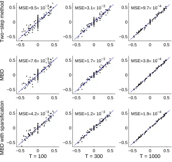
nonlinearity with exponent between 1.5 and 2.0 while keeping the original sign. The observations x(t)were then generated according to the model in Eq. (3). Various sample sizes (T = 100, 300, and 1000) were tested. We compared the performance of the two-stage method (Section 5.1), the method by MBD (Section 5.2) and the MBD-based method with the sparsity penalty (Section 5.3). In the last method, we set the penalization parameter in Eq. (14) asλ=log T to make its results con-sistent with those obtained by BIC. The densities of the independent components were adaptively estimated using the method in Pham and Garrat (1997). In each case, we repeated the experiments for 5 replications.
Fig. 1 shows the scatter plots of the estimated parameters (including the strictly lower triangular part of B0 and all entries of B1) versus the true ones. Different subplots correspond to different sample sizes or different methods. The mean square error (MSE) of the estimated parameters is also given in each subplot. One can see that as the sample sizes increases, all methods give better results. For each sample size, the method based on MBD is always better than the two-stage method, showing that the estimate by the MBD-based method is more efficient. Furthermore, due to the prior knowledge that many parameters are zero, the MBD-based method with the sparsity penalty performed best.
6. Assessment of the Significance of Causality
In practice, we also need to assess the significance of the estimated causal relations. While the spar-sification method in Section 5.3 is related to this goal, here we propose a more principled approach for testing the significance of the causal influences.
For the instantaneous effects xi(t)→xj(t) (i6= j), the significance of causality is obtained by
assessing if the entries of ˆB0are statistically significantly different from zero. For the lagged effects xi(t−τ)→xj(t) (i6=j,τ>0), however, one is often not interested in the significance of any single
coefficient in ˆBτ: More frequently one aims to find out if the total effect from xi(t−τ)to xj(t)is
significant.
We propose two simple statistics. One is a measure of instantaneous variance contributed by xi(t)to xj(t): S0(i← j) = [B0]2i j·var(xi(t))/var(xj(t)). If all time series have the same variance,
it is simplified to S0(i← j) = [B0]2i j. The other measures how strong the total lagged causal
in-fluence from xi(t)to xj(t)is; it is a measure of contributed variance from xi(t−τ),τ>0 to xj(t):
Slag(i← j) =var(∑τ>0[Bτ]i jxj(t−τ))/var(xj(t)). If all series xi(t) have the same variance and
are approximately temporally uncorrelated, the above statistic can be approximated by∑τ>0[Bτ]2
i j.
(Note that these quantities are not exactly proportions of variance explained because the explaining variables are not necessarily uncorrelated.)
The asymptotic distributions of these statistics under the null hypothesis (with no causal effects) are very difficult to derive, and they may also behave poorly in the finite sample case. Therefore, like in Diks and DeGoede (2001) and Theiler et al. (1992), we use bootstrapping with surrogate data to find the empirical distributions of each statistic under the null hypothesis. To generate the surrogate data under the null hypothesis, in each bootstrapping replication we “scramble” the original series xi(t), that is, each time series is randomly permuted in temporal order. We then calculate ˆS∗, the
−0.5 0 0.5 −0.5
0 0.5
Two−step method
MSE=9.5× 10⁻³
−0.5 0 0.5
−0.5 0
0.5 MSE=3.1× 10⁻³
−0.5 0 0.5
−0.5 0
0.5 MSE=9.7× 10⁻⁴
−0.5 0 0.5
−0.5 0 0.5
MBD
MSE=7.6× 10⁻³
−0.5 0 0.5
−0.5 0
0.5 MSE=1.7× 10⁻³
−0.5 0 0.5
−0.5 0
0.5 MSE=3.8× 10⁻⁴
−0.5 0 0.5
−0.5 0 0.5
T = 100
MBD with sparsification
MSE=4.2× 10⁻³
−0.5 0 0.5
−0.5 0 0.5
T = 300
MSE=1.2× 10⁻³
−0.5 0 0.5
−0.5 0 0.5
T = 1000
MSE=1.9× 10⁻⁴
Figure 1: Scatter plots of the estimated coefficients (y axis) versus the true ones (x axis) for different sample sizes and different methods.
of ˆS∗. Finally, we reject the null hypothesis if ˆS>c∗tα, where ˆS is the estimate of S for the original data.
7. Remarks on the Interpretation of the Parameters
In this section, we discuss how the autoregressive parameters are changed by taking into account the instantaneous effects, and how our model can be interpreted in the framework of Granger causality.
7.1 Interaction Between Instantaneous and Lagged Effects
While this phenomenon is, in principle, well-known in econometric literature (Swanson and Granger, 1997; Demiralp and Hoover, 2003; Moneta and Spirtes, 2006), Eq. (11) is seldom applied because estimation methods for B0have not been well developed. To our knowledge, no estimation method for B0 has been proposed which is consistent for the whole matrix without strong prior assumptions on B0.
Next we present some theoretical examples of how the instantaneous and lagged effects interact based on the formula in (11).
7.1.1 EXAMPLE1: ANINSTANTANEOUSEFFECTMAY SEEM TO BELAGGED
Consider first the case where the instantaneous and lagged matrices are as follows:
B0=
0 1 0 0
, B1=
0.9 0
0 0.9
.
That is, there is an instantaneous effect x2→x1, and no lagged effects (other than the purely autore-gressive xi(t−1)→xi(t)). Now, if an AR(1) model is estimated for data coming from this model,
without taking the instantaneous effects into account, we get the autoregressive matrix
M1= (I−B0)−1B1=
0.9 0.9
0 0.9
.
Thus, the effect x2→x1seems to be lagged although it is, actually, instantaneous. 7.1.2 EXAMPLE2: SPURIOUSEFFECTSAPPEAR
Consider three variables with the instantaneous effects x1→x2and x2→x3, and no lagged effects other than xi(t−1)→xi(t), as given by
B0=
0 0 0
1 0 0
0 1 0
, B1=
0.9 0 0
0 0.9 0
0 0 0.9
.
If we estimate an AR(1) model for the data coming from this model, we obtain
M1= (I−B0)−1B1=
0.9 0 0
0.9 0.9 0 0.9 0.9 0.9
.
This means that the estimation of the simple autoregressive model leads to the inference of a direct lagged effect x1→x3, although no such direct effect exists in the model generating the data, for any time lag.
A more reassuring result is the following: if the data follows the same causal ordering for all time lags, that ordering is not contradicted by the neglect of instantaneous effect. A rigorous definition of this property is the following.
Theorem 1 Assume that there is an ordering i(j),j=1. . .n of the variables such that no effect goes backward, that is,
(In the purely instantaneous case, existence of such an ordering is equivalent to acyclicity of the effects as noted in Section 2.2.) Then, the same property applies to the Mτ,τ≥1 as well. Conversely, if there is an ordering such that (15) applies to Mτ,τ≥1 and B0, then it applies to Bτ,τ≥1 as well.
Proof : When the variables are ordered in this way (assuming such an order exists), all the matrices Bτ are lower-triangular. The same applies to I−B0. Now, the product of two lower-triangular matrices is lower-triangular; in particular the Mτare also lower-triangular according to(11), which proves the first part of the theorem. The converse part follows from solving for Bτin (11) and the fact that the inverse of a lower-triangular matrix is lower-triangular.
What this theorem means is that if the variables really follow a single “causal ordering” for all time lags, that ordering is preserved even if instantaneous effects are neglected and a classic AR model is estimated for the data. Thus, there is some limit to how (11) can change the causal interpretation of the results.
7.2 Generalizations of Granger Causality
The classic interpretation of causality in instantaneous SEMs would be that xicauses xj if the(j,i)
-th coefficient in B0 is non-zero. On the other hand, in the time series context, the concept of Granger causality (Granger, 1969) formalizes causality as the ability to reduce prediction error. A simple operational definition of Granger causality can be based on the autoregressive coefficients Mτ: If at least one of the coefficients from xi(t−τ),τ≥1 to xj(t)is (significantly) non-zero, then
xi Granger-causes xj. This is because then the variable xi reduces the prediction error in xj in the
mean-square sense if it is included in the set of predictors, which is the very definition of Granger causality.
In light of the results in this paper, we can generalize the concept of Granger causality in two ways. First we can combine the two aspects of instantaneous and lagged effects. In fact, such a concept of instantaneous causality was already alluded to by Granger (1969), but presumably due to lack of proper estimation methods, that paper as well as most future developments considered mainly non-instantaneous causality. The second generalization is to measure prediction error by the information-theoretic definition of Section 4.3, essentially using entropy instead of mean squared error. These two generalization are independent of each other in the sense that we can use any one of them, omitting the other.
Both of these extensions are implicit in estimation of our model. Thus, we define that a variable xi causes xj if at least one of the coefficients Bτ(j,i), giving the effect from xi(t−τ) to xj(t), is
(significantly) non-zero for τ≥0. The condition for τ is different from Granger causality since
8. Real Data Experiments
We applied our model together with the estimation and testing method on both financial data and magnetoencephalography (MEG) data. In the former application, we used the sparsity penalty to select significant effects, while in the latter one, bootstrapping was used.
8.1 Application in Finance
First, we use the model in Eq. (3) to find the causal relations among several world stock indices. The chosen indices are Dow Jones Industrial Average (DJI) in USA, Nikkei 225 (N225) in Japan, Hang Seng Index (HSI) in Hong Kong, and the Shanghai Stock Exchange Composite Index (SSEC) in China. We used the daily dividend/split adjusted closing prices from 4th Dec 2001 to 11th Jul 2006, obtained from the Yahoo finance database. For the few days when the price is not available, we use simple linear interpolation to estimate the price. Denoting the closing price of the ith index on day t by Pi(t), the corresponding return is calculated by xi(t) =Pi(tP)i−(tP−i(1t)−1). The data for analysis
are x(t) = [x1(t), ...,x4(t)]T, with T =1200 observations.
We applied the MBD-based method with the sparsity penalty to x(t). The kurtoses of the es-timated disturbances ˆei are 3.9, 8.6, 4.1, and 7.6, respectively, implying that the disturbances are
non-Gaussian. We found that more than half of the coefficients in the estimated W0 and W1 are exactly zero due to sparsity penalty. Bb0 andBb1 were constructed based on W0 and W1, using the procedure given in Section 5.2. It was found thatBb0can be permuted to a strictly lower-triangular matrix, meaning that the instantaneous effects follow a linear acyclic causal model. Finally, based onBb0andBb1, one can plot the causal diagram, which is shown in Fig. 2.
Fig. 2 reveals some interesting findings. First, DJIt−1has significant impacts on N225tand HSIt,
which is a well-known fact in the stock market. Second, the causal relations DJIt−1→N225t→DJIt
and DJIt−1→HSIt →DJIt are consistent with the time difference between Asia and USA. That is,
the causal effects from N225tand HSIt to DJIt, although seeming to be instantaneous, may actually
be mainly caused by the time difference. Third, unlike SSEC, HSI is very sensitive to others; it is even strongly influenced by N225, another Asian index. Fourth, it may be surprising that there is a significant negative effect from DJIt−1 to DJIt; however, it is not necessary for DJIt to have
significant negative autocorrelations, due to the positive effect from DJIt−1to DJIt going through
N225t and HSIt.
8.2 Application on MEG Data
Second, we applied the proposed model on the magnitudes of brain sources obtained from magne-toencephalographic (MEG) signals to analyze their causal relationships. The raw recordings con-sisted of the 204 gradiometer channels measured by the Vectorview helmet-shaped neuromagne-tometer (Neuromag Ltd., Helsinki, Finland) in a magnetically shielded room at the Brain Research Unit of the Low Temperature Laboratory of the Aalto University School of Science and Technol-ogy. They were obtained from a healthy volunteer and lasted about 12 minutes. The data was downsampled to 75 Hz.
DJI
t-1N225
t-1HSI
t-1SSEC
t-1DJI
t0.12
N225
t0.42
HSI
t0.02
SSEC
t0.11
-0.15
0.35
0.21
-0.07
0.04
0.05
0.04
Figure 2: Results of application of our model to daily returns of the stock indices DJI, N225, HSI, and SSEC, with k=1 lag. Large coefficients (greater than 0.1) are shown in bold and red.
Next, we fitted an ordinary vector autoregressive model with 10 lags on the estimated sources, finding the corresponding innovation series which we denote by yi(t),i=1, ...,17. Our goal was
to analyze if there are some influences between the magnitudes of these innovations. We prefer to analyze the innovations because the innovations are approximately white both temporally and spatially, and thus we can analyze the magnitudes with no contamination by linear (auto)correlations of the source signals. The autoregressive model order 10 was chosen because it was the smallest order that gave approximately white innovations.
We then fitted the SVAR model on the logarithmically transformed magnitudes xi(t) =log(0.2+
|yi(t)|),i=1, ...,17. We determined the order k of our SVAR model by minimizing the AIC
crite-rion (Akaike, 1973), which is the negative log-likelihood of the MBD model plus a term measuring the complexity of the model. The log-likelihood involves the densities of the MBD outputs ˆei(t),
which were modelled by a mixture of three Gaussians. From the candidate orders between 0 and 20, we found that k=2 gave the minimum AIC.
After finding the estimate of the coefficients ˆBτ,τ=0,1,2 with the MBD-based approach, one can easily calculate the estimates of the statistics S0(i← j) and Slag(i← j). The bootstrapping
approach given in Section 6 was used to evaluate if these estimated statistics are significant. Here we need to test multiple hypotheses simultaneously; to reduce the type I error, we adopted the Bonferroni correction (Shaffer, 1995) for multiple testing correction. We used the significance level 5%. For both the instantaneous and lagged effects, one needs to perform 17×16=272 tests; therefore, the significance level for each individual test is then 0.05/272≈2×10−4. We used 104 replications for the bootstrapping.
For illustration, we give the empirical distribution of the statistics S0(7←14)and Slag(7←14),
as well as their estimated values for the original series xi(t), in Fig. 3. Clearly ˆS0(7←14) is
significant, while ˆSlag(7←14)is not.
0 0.2 0.4 0.6 0.8 1 1.2
x 10−4 0
1000 2000 3000 4000 5000 6000 7000 8000
Histogram of ˆS0(7←14) under null hypothesis
Critical value at 2× 10⁻⁴ level
ˆ S0(7←14)
0 0.2 0.4 0.6 0.8 1 1.2
x 10−4 0
1000 2000 3000 4000 5000 6000 7000 8000 9000
Histogram of ˆSlag(7←14) under null hypothesis
Critical value at 2× 10⁻⁴ level
ˆ Slag(7←14)
(a) (b)
Figure 3: Illustration of the empirical distribution of the statistics under the null hypothesis obtained by bootstrapping. (a) For the statistic S0(7←14). (b) For Slag(7←14).
9. Extensions of the Model
We have here assumed that B0is acyclic, as is typical in causal analysis. However, this assumption is only made because we do not know very well how to estimate a linear non-Gaussian Bayesian network (or SEM) in the cyclic case. If we have a method which can estimate cyclic models, we do not need the assumption of acyclicity in our combined model either; see Lacerda et al. (2008) for one proposal. We could just use such a new method in our two-stage method instead of LiNGAM, and nothing else would be changed. However, development of methods for estimating cyclic models is orthogonal to the main contribution of our paper in the sense that we can use any such new method to estimate the instantaneous model in our framework.
In formulating the likelihood we had to assume that the e(t)are independent and identically dis-tributed for different time points. However, in our two-stage estimation method, no such assumption was needed to guarantee consistency. In particular, the e(t)can be heteroscedastic, as long as e(t) and e(t′)are uncorrelated for t 6=t′ . In such a case, it might also be advantageous to change the LiNGAM estimation method so that the ICA part is replaced by methods estimating (4) explicitly based on temporal heteroscedasticity (Matsuoka et al., 1995; Hyv¨arinen, 2001; Pham and Cardoso, 2001); this is quite straightforward and necessitates no further changes in the method.
An interesting class of methods which is related to ours has been recently proposed by G´omez-Herrero et al. (2008). The idea is to combine blind source separation with a linear autoregressive model of the latent sources. The estimation of such a model can be accomplished by methods which are quite similar to our estimation methods, see also Haufe et al. (2009). However, the interpretation of the model is very different since, first, G´omez-Herrero et al. (2008) separate linear sources and analyze their (causal) connections whereas we analyze connections between the observed variables, and second, we estimate instantaneous causal influences whereas G´omez-Herrero et al. (2008) only estimate lagged ones.
10. Conclusion
We showed how non-Gaussianity enables estimation of a causal discovery model in which the linear effects can be either instantaneous or time-lagged. Like in the purely instantaneous case (Shimizu et al., 2006), non-Gaussianity makes the model identifiable without explicit prior assumptions on existence or non-existence of given causal effects. The theoretical developments are closely related to independent component analysis. The classic assumption of acyclicity was made, although it may not be necessary. From the practical viewpoint, an important implication is that considering instantaneous effects changes the coefficient of the time-lagged effects as well. We proposed meth-ods for computationally efficient estimation of the model, as well as for sparsification and testing of the model coefficients.
Acknowledgments
References
H. Akaike. Information theory and an extension of the maximum likelihood principle. Proc. 2nd International Symposium on Information Theory, pages 267–281, 1973.
F. Bach. Consistency of the group lasso and multiple kernel learning. Journal of Machine Learning Research, 9:1179–1225, 2008.
E. M. L. Beale and C. L. Mallows. Scale mixing of symmetric distributions with zero means. The Annals of Mathematical Statistics, 30(4):1145–1151, 1959.
K. A. Bollen. Structural Equations with Latent Variables. John Wiley & Sons, 1989.
J.-F. Cardoso and B. Hvam Laheld. Equivariant adaptive source separation. IEEE Trans. on Signal Processing, 44(12):3017–3030, 1996.
A. Chen and P. J. Bickel. Efficient independent component analysis. The Annals of Statistics, 34 (6):2824–2855, 2006.
A. Cichocki and S.-I. Amari. Adaptive Blind Signal and Image Processing: Learning Algorithms. Wiley, 2002.
P. Comon. Independent component analysis—a new concept? Signal Processing, 36:287–314, 1994.
S. Demiralp and K. D. Hoover. Searching for the causal structure of a vector autoregression. Oxford Bulletin of Economics and Statistics, 65 (supplement):745–767, 2003.
C. Diks and J. DeGoede. A general nonparametric bootstrap test for granger causality. In H. Broer and B. Krauskopf nd G. Vegter, editors, Global Analysis of Dynamical Systems, pages 391–403 (Chapter 16). Taylor & Francis, London, 2001.
R. F. Engle, editor. ARCH: Selected Readings. Oxford University Press, 1995.
K. J. Friston, L. Harrison, and W. Penny. Dynamic causal modelling. NeuroImage, 19(4):1273– 1302, 2003.
G. G´omez-Herrero, M. Atienza, K. Egiazarian, and J.L. Cantero. Measuring directional coupling between EEG sources. NeuroImage, 43:497–508, 2008.
C. W. J. Granger. Investigating causal relations by econometric models and cross-spectral methods. Econometrica, 37:424–438, 1969.
R. Hari and R. Salmelin. Human cortical oscillations: a neuromagnetic view through the skull. Trends in Neuroscience, 20:44–49, 1997.
S. Haufe, R. Tomioka, G. Nolte, K.-R. M¨uller, and M. Kawanabe. Modeling sparse connectivity between underlying brain sources for EEG/MEG. 2009. Arxiv preprint.
A. Hyv¨arinen. Blind source separation by nonstationarity of variance: A cumulant-based approach. IEEE Transactions on Neural Networks, 12(6):1471–1474, 2001.
A. Hyv¨arinen. Fast and robust fixed-point algorithms for independent component analysis. IEEE Transactions on Neural Networks, 10(3):626–634, 1999.
A. Hyv¨arinen and E. Oja. Independent component analysis by general nonlinear Hebbian-like learn-ing rules. Signal Processlearn-ing, 64(3):301–313, 1998.
A. Hyv¨arinen, J. Karhunen, and E. Oja. Independent Component Analysis. Wiley Interscience, 2001.
A. Hyv¨arinen, S. Shimizu, and P. O. Hoyer. Causal modelling combining instantaneous and lagged effects: an identifiable model based on non-Gaussianity. In Proc. Int. Conf. on Machine Learning (ICML2008), pages 424–431, Helsinki, Finland, 2008.
A. Hyv¨arinen, P. Ramkumar, L. Parkkonen, and R. Hari. Independent component analysis of short-time Fourier transforms for spontaneous EEG/MEG analysis. NeuroImage, 49(1):257–271, 2010.
J. Karvanen and V. Koivunen. Blind separation methods based on pearson system and its extensions. Signal Processing, 82(4):663–573, 2002.
J. Kim, W. Zhu, L. Chang, P. M. Bentler, and T. Ernst. Unified structural equation modeling ap-proach for the analysis of multisubject, multivariate functional MRI data. Human Brain Mapping, 28:85–93, 2007.
G. Lacerda, P. Spirtes, J. Ramsey, and P. O. Hoyer. Discovering cyclic causal models by independent components analysis. In Proc. 24th Conf. on Uncertainty in Artificial Intelligence (UAI2008), Helsinki, Finland, 2008.
R. W. Liu and H. Luo. Direct blind separation of independent non-Gaussian signals with dynamic channels. In Proc. Fifth IEEE Workshop on Cellular Neural Networks and their Applications, pages 34–38, London, England, April 1998.
K. Matsuoka, M. Ohya, and M. Kawamoto. A neural net for blind separation of nonstationary signals. Neural Networks, 8(3):411–419, 1995.
A. Moneta and P. Spirtes. Graphical models for the identification of causal structures in multivariate time series models. In Proc. Joint Conference on Information Sciences, Kaohsiung, Taiwan, 2006.
R. Opgen-Rhein and K. Strimmer. From correlation to causation networks: a simple approximate learning algorithm and its application to high-dimensional plant gene expression data. BMC Systems Biology, 1(37), 2007.
J. Pearl. Causality: Models, Reasoning, and Inference. Cambridge University Press, 2000.
D.-T. Pham and J.-F. Cardoso. Blind separation of instantaneous mixtures of non stationary sources. IEEE Trans. Signal Processing, 49(9):1837–1848, 2001.
A. Roebroeck, E. Formisano, and R. Goebel. Mapping directed influence over the brain using Granger causality and fMRI. NeuroImage, 25(1):230–242, 2005.
J. P. Shaffer. Multiple hypothesis testing. Annual Review of Psychology, 46:561–584, 1995.
S. Shimizu, P. O. Hoyer, A. Hyv¨arinen, and A. Kerminen. A linear non-Gaussian acyclic model for causal discovery. J. of Machine Learning Research, 7:2003–2030, 2006.
P. Spirtes, C. Glymour, and R. Scheines. Causation, Prediction, and Search. Springer-Verlag, 1993.
N. R. Swanson and C. W. J. Granger. Impulse response functions based on a causal approach to residual orthogonalization in vector autoregression. J. of the Americal Statistical Association, 92: 357–367, 1997.
J. Theiler, S. Eubank, A. Longtin, B. Galdrikian, and J. Farmer. Testing for nonlinearity in time series: the method of surrogate data. Physica D, 58:77–94, 1992.
K. Zhang and A. Hyv¨arinen. Causality discovery with additive disturbances: An information-theoretical perspective. In Proc. European Conference on Machine Learning (ECML2009), pages 570–585, 2009.
K. Zhang, H. Peng, L. Chan, and A. Hyv¨arinen. ICA with sparse connections: Revisited. In Proc. Int. Conference on Independent Component Analysis and Blind Signal Separation (ICA2009), pages 195–202, Paraty, Brazil, 2009.