Using Machine Learning to Guide Architecture Simulation
Greg Hamerly [email protected]
Department of Computer Science Baylor University
One Bear Place #97356 Waco, TX 76798-7356, USA
Erez Perelman [email protected]
Jeremy Lau [email protected]
Brad Calder [email protected]
Department of Computer Science and Engineering University of California, San Diego
9500 Gilman Drive
La Jolla, CA 92093-0404, USA
Timothy Sherwood [email protected]
Department of Computer Science University of California, Santa Barbara Santa Barbara, CA 93106, USA
Editor: Haym Hirsh
Abstract
An essential step in designing a new computer architecture is the careful examination of dif-ferent design options. It is critical that computer architects have efficient means by which they may estimate the impact of various design options on the overall machine. This task is compli-cated by the fact that different programs, and even different parts of the same program, may have distinct behaviors that interact with the hardware in different ways. Researchers use very detailed simulators to estimate processor performance, which models every cycle of an executing program. Unfortunately, simulating every cycle of a real program can take weeks or months.
To address this problem we have created a tool called SimPoint that uses data clustering algo-rithms from machine learning to automatically find repetitive patterns in a program’s execution. By simulating one representative of each repetitive behavior pattern, simulation time can be reduced to minutes instead of weeks for standard benchmark programs, with very little cost in terms of accu-racy. We describe this important problem, the data representation and preprocessing methods used by SimPoint, the clustering algorithm at the core of SimPoint, and we evaluate different options for tuning SimPoint.
Keywords: k-means, random projection, Bayesian information criterion, simulation, SimPoint
1. Introduction
the full execution of a single benchmark can take weeks or months to complete, and nearly all in-dustry standard benchmarks require the execution of a suite of programs. For example, the SPEC benchmark suite consists of 26 different programs, requiring the execution of a combined total of approximately 6 trillion instructions. Still worse, architecture researchers need to simulate each benchmark over a variety of different architectural configurations and design options, to find the set of features that provides an appropriate trade-off between performance, complexity, area, and power. The same program binary, with the exact same input, may be run hundreds or thousands of times to examine how, for example, the effectiveness of a given architecture changes with its cache size. Researchers need techniques which can reduce the number of machine-months required to estimate the impact of an architectural modification without introducing an unacceptable amount of error or excessive simulator complexity. We present a method, distributed as a software package called SimPoint, which can meet this need by exploiting the structured way in which individual programs change behavior over time.
As a program executes its behavior changes. These changes are not random, but rather are often structured as sequences of a small number of recurring behaviors, which we term phases. Identifying this repetitive and structured behavior can be of great benefit, since it means we only need to sample each unique behavior once to create a complete representation of the program’s execution. This is the underlying philosophy of SimPoint (Sherwood et al., 2001, 2002; Perelman et al., 2003; Biesbrouck et al., 2004; Lau et al., 2004, 2005b). SimPoint intelligently chooses a very small set of samples from an executed program called simulation points that, when simulated and weighted appropriately, provide an accurate picture of the complete execution of the program. Simulating in detail only these carefully chosen simulation points can save hours of simulation time over a random sampling of the program, while still providing the accuracy needed to make reliable decisions based on the outcome of the cycle level simulation.
Before we developed SimPoint, architecture researchers would simulate SPEC programs for 300 million instructions from the start of execution, or fast forward 1 billion instructions to try to get past the initialization part of the program. These techniques can result in error rates of up to 3736% in predicting the architecture metrics we wish to measure. SimPoint achieves very low error rates (2% average error, 8% maximum error for the results in this paper) and on average reduces simulation time by a factor of 1,500, compared to simply simulating the whole program. This approach is now used by researchers in the architecture community, and companies such as Intel (Patil et al., 2004). This paper shows how repetitive phase behavior can be found in programs through machine learning and describes how SimPoint automatically finds these phases and picks simulation points.
2. The Application - Simulation
In this section we explain the tools modern computer architects use to evaluate designs and the methods we use to evaluate our solutions.
2.1 Background
Processor architecture research quantifies the effectiveness of a design by executing a program on a software model of the architecture design called an architecture simulator. It is difficult to accu-rately compare studies that provide results for different sets of programs. To set a standard in the community, the Standard Performance Evaluation Corporation (SPEC) was established to provide a collection of benchmarks to evaluate processor performance. In the same manner, the architecture simulator needs to have a common baseline. SimpleScalar (Burger and Austin, 1997) is a cycle level processor simulator that has become a standard model for architecture research.
2.1.1 SPEC CPU BENCHMARKS
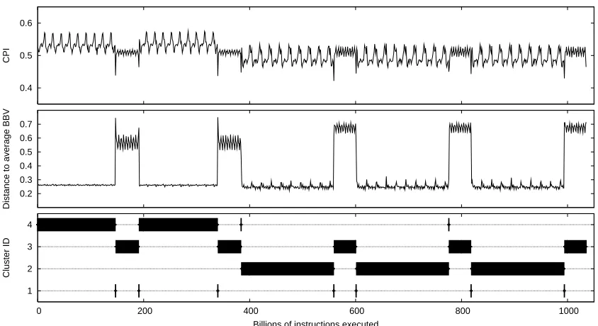
The SPEC CPU2000 benchmark suite has 26 programs, of which 12 are integer programs (primary execution is of integer instructions) and 14 are floating-point programs (primary execution is of floating-point instructions). The benchmark suite is chosen to stress a processor across its many components in a rigorous manner. Each program in the suite has 3 different inputs: test, train, and reference, which respectively correspond to a short test, a more representative training, and a full reference run. The test, train and reference inputs typically execute on the order of a few million, a few billion, and hundreds of billions of instructions respectively. Tables 1 and 2 show all the SPEC CPU2000 benchmarks, divided into integer and floating-point programs. The tables provide a high level description of each benchmark, its source language, and the number of instructions executed (in billions) with the reference and test inputs. These programs were compiled for the Alpha Instruction Set Architecture (ISA) with full optimizations. On average, the reference inputs
execute for 223 billion instructions. The programparserhas the maximum instruction count at
546 billion instructions.
SPEC periodically releases a benchmark suite to evaluate current and future processors. To keep up with the ever increasing rate of processor speeds, SPEC has significantly increased the duration of benchmark execution from the previous suite release in 1995 to the current release of 2000. This is because the reference input needs to run long enough to achieve a valid timing for the benchmark run. This means that with current and future speeds that future releases of the SPEC benchmark suite will need to execute on the order of trillions of instructions for the reference inputs.
2.1.2 SIMPLESCALAR
mod-Benchmark Ref Length Test Length Language Category
bzip2 143 8.82 C Compression
crafty 191 4.26 C Game Playing: Chess
eon 80 0.09 C++ Computer Visualization
gap 269 1.17 C Group Theory, Interpreter
gcc 46 2.02 C C Programming Language Compiler
gzip 84 3.37 C Compression
mcf 61 0.26 C Combinatorial Optimization
parser 546 4.20 C Word Processing
perlbmk 111 2.0 C PERL Programming Language
twolf 346 0.26 C Place and Route Simulator
vortex 118 9.81 C Object-oriented Database
vpr 84 0.69 C FPGA Circuit placement and routing
Table 1: SPEC CPU2000 Integer Benchmarks (lengths in billions of instructions)
Benchmark Ref Length Test Length Language Category
ammp 326 5.49 C Computational Chemistry
applu 223 0.18 Fortran 77 Parabolic / Elliptic Partial Differential Equations
apsi 347 5.28 Fortran 77 Meteorology: Pollutant Distribution
art 41 1.48 C Image Recognition / Neural Networks
equake 131 1.44 C Seismic Wave Propagation Simulation
facerec 211 4.12 Fortran 90 Image Processing: Face Recognition
fma3d 268 0.00 Fortran 90 Finite-element Crash Simulation
galgel 409 4.34 Fortran 90 Computational Fluid Dynamics
lucas 142 3.71 Fortran 90 Number Theory / Primality Testing
mesa 281 2.88 C 3-D Graphics Library
mgrid 419 16.77 Fortran 77 Multi-grid Solver: 3D Potential Field
sixtrack 470 8.59 Fortran 77 High Energy Nuclear Physics Accelerator Design
swim 225 0.43 Fortran 77 Shallow Water Modeling
wupwise 349 3.63 Fortran 77 Physics / Quantum Chromodynamics
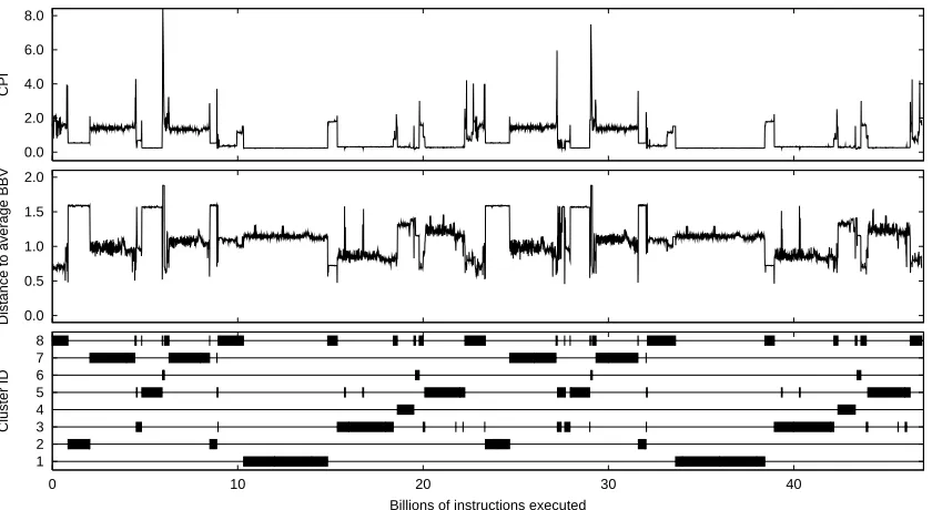
I Cache 16k 2-way set-associative, 32 byte blocks, 1 cycle latency D Cache 16k 4-way set-associative, 32 byte blocks, 2 cycle latency L2 Cache 1Meg 4-way set-associative, 32 byte blocks, 20 cycle latency Main Memory 150 cycle latency
Branch Pred hybrid - 8-bit gshare w/ 8k 2-bit predictors + a 8k bimodal predictor O-O-O Issue out-of-order issue of up to 8 operations per cycle, 128 entry re-order buffer Mem Disambig load/store queue, loads may execute when all prior store addresses are known Registers 32 integer, 32 floating point
Func Units 8-integer ALU, 4-load/store units, 2-FP adders, 2-integer MULT/DIV, 2-FP MULT/DIV
Virtual Mem 8K byte pages, 30 cycle fixed TLB miss latency after earlier-issued instructions complete
Table 3: Baseline Simulation Model.
els and provides the highest level of execution detail. The architecture research community uses SimpleScalar extensively, and today it is considered a standard architecture simulator.
The different models in SimpleScalar each have a stable execution rate. The fastest model, sim-fast, executes on the order of tens of billion instructions per hour on a 1 GHz machine. The slowest yet most accurate model, sim-outorder, executes on the order of hundreds of million instructions per hour, which is several orders of magnitude slower than the native hardware. It would take months of computation time to simulate the entire SPEC benchmark suite with sim-outorder. What makes matters worse is that researchers need to evaluate many different hardware configurations to measure the effectiveness of a design. This enormous turnaround time for a study makes simulating the full benchmark infeasible, and the majority of researchers only simulate a few hundred million instructions from each benchmark.
2.2 Methodology
For this study, we performed our analysis for the complete set of SPEC CPU2000 programs for mul-tiple inputs using the Alpha binaries from the SimpleScalar website. We collect all of the frequency vector profiles, described in Section 4, using SimpleScalar. To generate our baseline results, we executed all programs from start to completion using SimpleScalar, gathering the hardware metrics. The baseline microarchitecture model is detailed in Table 3.
To examine the accuracy of our approach we provide results in terms of CPI prediction error and k-means variance (since SimPoint uses k-means clustering). The CPI prediction error is the percent difference between CPI predicted using only simulation points chosen by SimPoint and the baseline (true) CPI of the complete execution of the program. The k-means variance is the sum-of-squared distances between every clustered point and its closest center, which is the criterion k-means optimizes.
3. Defining Phase Behavior
Since phases are a way of describing the recurring behavior of a program executing over time, we begin by describing phase analysis with a demonstration of the time-varying behavior (Sherwood
and Calder, 1999) of two programs from the SPEC 2000 benchmark suite, gcc and gzip. To
1 2 3 4
0 200 400 600 800 1000
Cluster ID
Billions of instructions executed 0.2
0.3 0.4 0.5 0.6 0.7
Distance to average BBV
0.4 0.5 0.6
CPI
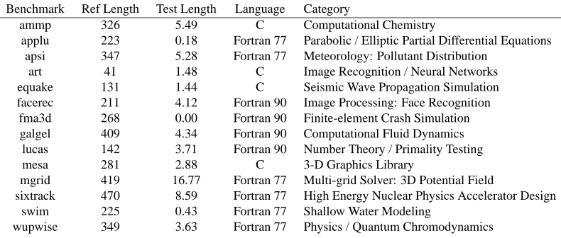
Figure 1: These plots show the relationship between measured performance (CPI) and code usage
for the programgzip-graphic, and SimPoint’s ability to capture phase information by
only looking at what code is being executed. For each of the three plots, the horizontal axis represents the execution of the program over time, and each point plotted represents one 10-million instruction interval. The top plot shows the CPI for the executing program. The middle plot shows the distance of each interval’s basic block vector (explained in Section 4) to the “target vector”, which is a basic block vector that represents the entire program’s execution. The target vector is a signature of the program’s overall average behavior, and this plot shows how similar the code of each part of the program is to the overall behavior of the program, lower meaning more similar. The bottom plot shows how SimPoint classifies each interval into one of four phases. The phase transitions correspond to changes in the CPI in the top graph, though SimPoint does not use metrics like CPI to classify intervals.
to finish. Each program executes many billions of instructions, and gathering these results took several machine-months of simulation time. The behavior of each program is shown in the top graphs of Figures 1 and 2. Each top graph shows how the CPI rate changes for these two programs over time. CPI is a commonly used metric in the processor architecture community for measuring processor performance. Each point on the graph represents the average CPI taken over a window (we call it an interval) of 10 million executed instructions. These graphs show that programs are fairly complex, changing behaviors frequently.
1 2 3 4 5 6 7 8
0 10 20 30 40
Cluster ID
Billions of instructions executed 0.0
0.5 1.0 1.5 2.0
Distance to average BBV
0.0 2.0 4.0 6.0 8.0
CPI
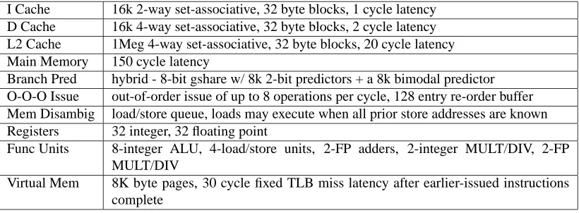
Figure 2: These plots show the relationship between measured performance (CPI) and code usage
for the programgcc-166, and SimPoint’s ability to capture phase information by only
looking at what code is being executed. For each of the three plots, the horizontal axis represents the execution of the program over time, and each point plotted represents one 10-million instruction interval. The top plot shows the CPI for the executing program. The middle plot shows the distance of each interval’s basic block vector to the “target vector”, which is a basic block vector (explained in Section 4) that represents the entire program’s execution. The target vector is a signature of the program’s overall average behavior, and this plot shows how similar the code of each part of the program is to the overall behavior of the program, lower meaning more similar. The bottom plot shows how SimPoint classifies each interval into one of eight phases. The phase transitions correspond to changes in the CPI in the top graph, though SimPoint does not use metrics like CPI to classify intervals.
direction (Sherwood and Calder, 1999; Sherwood et al., 2002). These corresponding changes are due to underlying changes in program execution.
The underlying methodology used in this work is the ability to automatically identify these underlying program changes without relying on architectural metrics. To ground our discussion in a common vocabulary, the following is a list of definitions to describe program behavior and its automated classification.
• Interval – To perform our analysis we break a program’s execution up into non-overlapping
in the program’s execution, the third interval represents instructions 200 to 300 million, etc. For the results in this work all intervals are chosen to be the same length, as measured in the number of instructions committed within an interval. This is usually 1, 10, or 100 million instructions, as used by Perelman et al. (2003).
• Similarity – A similarity metric measures the similarity in behavior between two intervals of
a program’s execution, and is specific to the representation of those intervals.
• Phase – A set of intervals within a program’s execution that all have similar behavior,
regard-less of temporal adjacency. A phase may be made up of intervals which are disjoint in time; we would call this a phase with a repeating behavior. A “well-formed” phase should have intervals with similar behavior across various architecture metrics (e.g. CPI, cache misses, branch misprediction). In this paper we consider the terms ‘cluster’ and ‘phase’ to be equiv-alent.
• Phase Classification – Using machine learning to group intervals from a program/input pair
into phases (clusters) with similar behavior.
4. The Strong Correlation Between Code and Performance
In this section we describe how we identify phase behavior in an architecture independent fashion.
4.1 Using an Architecture-Independent Metric for Phase Classification
To find program phases, we need a notion of how similar are two different parts of a program’s execution. In creating this metric it is advantageous to not rely on hardware-based statistics such as cache miss rates or performance (i.e. CPI), since using these would tie the phases to those statistics which change depending on the architecture configuration. If such statistics were used, the phases would need to be re-analyzed every time there was a change to some architectural parameter (either statically if the size of the cache changed, or dynamically if some policy changes adaptively). This is not acceptable, since our goal is to find a set of samples that can be used across an architecture design space exploration, where many of these parameters may change. To address this, we need a metric that is independent of any particular hardware-based statistic, but still relates to the fundamental changes in behavior like those shown in the top graphs of Figures 1 and 2.
An effective way to design such a metric is to base it on the behavior of a program in terms of the code that is executed over time. We have shown that there is a very strong correlation (Lau et al., 2005b) between the set of paths executed in a program and the time-varying architectural behavior observed. The intuition behind this is that the executed code determines the behavior of the program. With this idea it is possible to find the phases in programs using only a metric related to how the code is being exercised (i.e. both what code is touched and how often). The central idea behind SimPoint is that it can find the phase behavior shown in the top graphs of Figures 1 and 2 by examining only the frequency with which the code parts (e.g., basic blocks) are executed over time.
4.2 Basic Block Vector
code (e.g. a contiguous set of instructions) that is executed from start to finish with one entry and one exit. The metric we will use for comparing two time intervals in a program is based on the differences in the execution frequencies for each basic block executed during those two intervals. The intuition behind this is that the behavior of the program at a given time is directly related to the code it is executing during that interval, and basic block vectors provide us with this information.
A program, when run for any interval of time, will execute each basic block a certain number of times. Knowing this information provides a code signature for that interval of execution, and shows where the application is spending its time in the code. The basic idea is that knowing the basic block distribution for two different intervals gives two separate signatures which we can then compare to find out how similar the intervals are to one another. If the signatures are similar, then the two intervals spend about the same amount of time in the same code, and the performance of those two intervals should be similar.
We represent a basic block vector as a one-dimensional array, with one element in the array for each static basic block in the program. Each interval in an executed program is represented by one BBV, and at the beginning of each interval, its corresponding BBV has all zeros. During each interval, we count the number of times each basic block has been entered, and record that number into the corresponding element in the vector. This number is weighted by the number of instructions in the basic block, since we want every individual instruction to have the same influence. Therefore, each element in the array is the count of how many times its corresponding basic block has been entered during an interval of execution, multiplied by the number of instructions in that basic block. For example, if the 50th basic block has one instruction and is executed 15 times in an interval, then bbv[50] = 15 for that interval. At the end of an interval’s execution, we normalize the BBV to sum to 1.
We call the vectors used to guide phase analysis Frequency Vectors, of which basic block vec-tors are one type. Frequency vecvec-tors can represent basic blocks, branch edges, or any other type of program related structure which provides a representative summary of a program’s behavior for each interval of execution. We recently examined frequency vector structures other than basic block vectors for the purpose of phase classification. We have looked at frequency vectors for data, loops, procedures, register usage, instruction mix, and memory behavior (Lau et al., 2004). We found that using register usage vectors, which simply counts for a given interval the number of times each register is defined and used, provides similar accuracy to using basic block vectors. In addition, us-ing only loop and procedure branch execution frequencies performs almost as well as usus-ing the full basic block information. We also found, for SPEC 2000 programs, that creating frequency vectors by including both code and data access patterns into the vectors did not improve classification over just using code (Lau et al., 2004).
4.3 Basic Block Vector Difference
In order to find patterns in a program we must first have some way of comparing the similarity of two basic block vectors. The operation should take two basic block vectors and return a single number corresponding to how similar (or different) they are.
we examine in this paper uses Euclidean distance as the metric for comparing basic block vectors, since it is based on k-means. For on-the-fly phase analysis (e.g. predicting phases during computa-tion), the Manhattan distance is more efficiently implemented in hardware. It has been shown to be useful in previous work in online phase prediction (Sherwood et al., 2003; Lau et al., 2005c).
4.4 Showing the Correlation Between Code Signatures and Performance
For a detailed study showing that there is a strong correlation between executed code and real performance, please see Lau et al. (2005b). The top two graphs of Figure 2 give one illustration of this correlation by showing the time-varying CPI and BBV distance graphs next to each other for
gcc-166. The top graph plots the CPI for each interval executed (at 10M interval length) showing how the program’s CPI varies over time. Similarly, the BBV distance graph plots for each interval the Manhattan distance of the BBV (code signature) for that interval from the whole program’s target vector. The whole program’s target vector is a BBV that comes from viewing the whole
program as a single interval. The same information is also provided forgzipin the top two graphs
of Figure 1. These graphs show that changes in CPI have corresponding changes in code signatures, which is one indication of strong phase behavior for these applications.
These graphs show a strong correlation between code changes and CPI changes even for
com-plex programs likegcc. The graphs forgzip show that phase behavior can be found even if the
intervals’ CPIs have small variance. This brings up an important point about classifying intervals based on code similarity rather than based on similarity of CPI or some other hardware metric. As-sume we have two intervals with different code signatures but they have very similar CPIs because both of their working sets fit completely in the cache. During a design space exploration search, as the cache size changes, their CPIs may differ dramatically if one of them no longer fits into the cache. This is why it is important to perform the phase analysis by comparing the code signatures independent of the underlying architecture. We have found that the BBV code signatures correctly identify differences like these, which cannot be seen by looking at just the CPI.
4.5 Basic Block Similarity Matrix
Now that we have methods of comparing program execution intervals, we can use them for finding phase-based behavior. A phase of program behavior can be defined in several ways. Past definitions were built around the idea of a phase being a contiguous interval of execution during which a measured program metric is relatively stable. We extend this notion of a phase to include all similar sections of execution regardless of temporal adjacency. Thus, a phase may appear several times in the execution of a program.
A key observation from this paper is that the phase behavior seen in any program metric is a function of the code being executed. Because of this we can use the comparison between the basic block vectors to get an idea of how closely related any other metrics will be between those two intervals.
To find how all intervals of execution relate to one another we create a basic block similarity
matrix for a program/input pair. The similarity matrix is an upper-triangular n×n matrix, where
n is the number of intervals in the program’s execution. An entry at(x,y)in the matrix represents
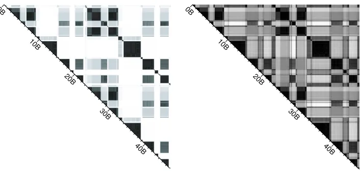
Figures 3 (left and right) and 4 (left) shows the similarity matrices forgzip,bzip, andgccusing the Manhattan distance. The diagonal of the matrix represents the program’s execution over time from start to completion. The darker the points, the more similar the intervals are (the Manhattan distance is closer to 0), and the lighter they are the more different they are (the Manhattan distance is closer to the maximum value — which is 2 since each vector is normalized to sum to 1).
Consider the points along the matrix diagonal. The top left corner of each matrix is the start
of program execution (0,0), and the bottom right is the point (n−1,n−1) (end of execution).
Each interval is perfectly similar to itself, so the points on the diagonal are all dark. Starting from a point on the diagonal, you can compare how its corresponding interval relates to its neighbors forward (backward) in execution by tracing horizontally (vertically) from that point. For example,
to compare a given interval x with the interval at x+m, start at the point(x,x)on the matrix and
trace to the right until you reach(x,x+m).
Let us first examinegzipbecause it has behaviors that are evident at such a large scale that they
are easy to see. An interval taken from 70 billion instructions into execution in Figure 3 (left) is directly in the middle of a large phase shown by the triangle of dark points that surround this point. This means that this interval is very similar to its neighbors both forward and backward in time. We can also see that the intervals at 50 billion and 90 billion instructions are also very similar to the program behavior at 70 billion instructions. While it may be hard to see in a printed version, the intervals around 70 billion instructions are similar to the intervals around 10 billion and 30 billion instructions, and even more similar to those around 50 and 90 billion instructions.
Overall, Figure 3 (left) shows that the phase behavior seen in the similarity matrix lines up quite closely with the behavior of the program seen in the top graph of Figure 1, with 5 large regions of self-similar behavior (the first 2 being different from the last 3) each divided by a small region of self-similar behavior. All of the small self-similar regions are also very similar to each other.
The similarity matrix forbzip (shown on the right of Figure 3) is very interesting. Bziphas
complicated behavior, with two large parts to its execution: compression and decompression. This can readily be seen in the figure as the large dark triangular and square patches. The interesting
thing aboutbzipis that even within each of these sections of execution there is complex behavior.
This, as will be shown later, makes the behavior ofbzipimpossible to capture using only one small
contiguous section of execution.
An even more complex case for finding phase behavior is gcc, which is shown on the left of
Figure 4 ( the matrix on the right of that figure will be explained in more detail in Section 5.1.1).
The left matrix shows thatgccdoes have regular behavior. Even for such a complex program, we
see that there is common code shared between sections of execution, such as the intervals around 13 billion instructions and 36 billion instructions. In fact the strong dark diagonal line cutting through the matrix indicates that there is large-scale repetition between the first half and second half of the program. By analyzing the graph we can see that code at each interval x is very similar to interval (x+23.6B instructions).
5. Automatically Finding Phase Behavior
0B
20B
40B
60B
80B
100B 0B
50B
100B
Figure 3: Basic block similarity matrix for the programs gzip-graphic (shown left) and
bzip-graphic(shown right). The diagonal of the matrix represents the program’s exe-cution from beginning to end, with units in billions of instructions. The darker the points, the more similar the intervals are (the Manhattan distance is closer to 0), and the lighter the points the more different they are (the Manhattan distance is closer to 2).
0B
10B
20B
30B
40B
0B
10B
20B
30B
40B
Figure 4: The original similarity matrix for the programgcc-166(left), and the similarity matrix
for the projection ofgcc-166(right). The figure on the left uses the original basic block
5.1 Using Clustering for Phase Classification
A primary goal of SimPoint is to have an automated way of extracting phase information from programs. Data clustering algorithms from unsupervised machine learning have been shown to be very effective at breaking the complete execution of a program into phases that have similar frequency vectors (Sherwood et al., 2002). Because the frequency vectors correlate to the overall performance of the program, grouping intervals based on their frequency vectors produces phases that are similar not only in the distribution of program structures used, but also in every other architecture metric measured, including overall performance.
The goal of clustering is to divide a set of points into clusters such that points within each cluster are similar to one another (by some metric), and points in different clusters are different from one another. We use the machine learning term ‘cluster’ and the architecture term ‘phase’ to express the same concept.
The k-means algorithm (MacQueen, 1967) is an efficient and well-known clustering algorithm, which we use to split program intervals into phases. Prior to clustering, we use random linear projection (Dasgupta, 2000) to reduce the dimension of the input vectors. One drawback of the k-means algorithm is that it requires the number of clusters k as an input to the algorithm, but we do not know beforehand what value is appropriate. To address this, we run the algorithm for several values of k, and then use a penalized likelihood score to guide our final choice for k. Taken to the extreme, if every interval of execution is given its very own cluster, then every cluster will have homogeneous behavior. Our goal is to choose a clustering with a minimum number of clusters which still models the program behavior well.
The following steps summarize the SimPoint phase clustering algorithm at a high level.
1. Profile the program by dividing the program’s execution into contiguous intervals of fixed length (e.g., 1 million, 10 million, or 100 million instructions). For each interval, collect a frequency vector tracking the program’s use of some program structure (basic blocks, branch edges, loops, register usage, etc.). Each frequency vector is normalized so that the sum of all the elements equals 1.
2. Reduce the dimensionality of the frequency vector data to a much smaller number of dimen-sions using random linear projection. Using projected data speeds up the k-means algorithm significantly and reduces the memory requirements by several orders of magnitude while pre-serving the essential similarity information.
3. Run the k-means clustering algorithm on the projected data with values of k in the range from 1 to K, where K is a user-prescribed maximum number of phases that can be detected. Each run of k-means produces a clustering, which is a partition of the data into k different phases/clusters. Each run of k-means begins with a random initialization step, which requires a random seed.
4. To compare and evaluate the different clusters formed for different k, we use the Bayesian Information Criterion (BIC) as a measure of the “goodness of fit” of a clustering to a data set. A high BIC score indicates the clustering is a good fit to the data. For each clustering (k∈ {1,2, . . . ,K}), the fitness of the clustering is scored using the BIC.
The above algorithm groups intervals into phases. This algorithm has several important param-eters: interval length, projected dimension, the maximum number of clusters K, how the BIC is to be used to select the best clustering, etc. Each must be tuned to create accurate and representative simulation points using SimPoint. We discuss these parameters in more detail later in this paper.
5.1.1 RANDOMPROJECTION
For this clustering problem, we have to address the problem of high dimensionality. Many clustering algorithms suffer from the so-called “curse of dimensionality,” which refers to the fact that finding an optimal clustering is intractable as the number of dimensions increases. One problem is that ge-ometric optimizations that give significant speedup in low-dimensional data often have the opposite effect in high dimensions (e.g. k-d trees for speeding up nearest neighbor queries). For basic block vectors, the number of dimensions is the number of executed basic blocks in the program, which ranges from 2,756 to 102,038 for the SPEC benchmark suite, and could grow into the millions for very large programs. For example, one Microsoft application we studied consisted of over 800,000 basic blocks, which is representative of desktop applications. Another practical problem is that the running time and memory requirements of k-means depend on the dimension of the data, making the algorithm slow if the dimension grows too large. Also, we observe that k-means tends to get stuck easily in sub-optimal solutions if the dimension is too high. This is evidenced by the small number of iterations k-means requires to converge on high-dimensional data, as we have observed on this data. The algorithm does not improve much over its initialization.
Two broad methods of reducing the dimension of data are dimension selection and dimension reduction. Dimension selection simply removes some of the dimensions, based on a measure of goodness of each dimension for describing the data. However, this can throw away a lot of infor-mation in the dimensions which are ignored. Also, in finding a measure to select useful dimensions is not as clear for unsupervised learning as for supervised learning. Dimension reduction reduces the number of dimensions by creating a new lower-dimensional space and then projecting each data point into the new space (where the new space’s dimensions are not necessarily related to the old space’s dimensions).
For this work we use random linear projection (Dasgupta, 2000) to create a new low-dimensional space into which we orthogonally project the data. This is a simple and fast technique that is very effective at reducing the number of dimensions while retaining the essential structure of the data. There are two steps to projecting a data set down to a lower-dimensional version. Consider a data
set X which is represented as a matrix of n×d real values, where n is the number of vectors, and
d is the original dimension. We want a low-dimension version X0 which is n×d0, where d0 is the
projected number of dimensions. To create X0, we do the following:
• Create a projection matrix P size d×d0. Fill each entry in the matrix with a random value
chosen uniformly in[−1,1].
• Use a matrix multiplication to obtain X0=X×P.
k Gaussian clusters can be projected into only O(log k)dimensions while retaining the approximate level of separation between clusters.
Principal components analysis (PCA) is a widely-used method for dimension reduction based on directions of high variance. However, performing PCA on a d-dimensional data set requires
O(d3)operations, which is too expensive for data sets of the size we are considering here that can
have hundreds of thousands of dimensions. Constructing the random projection matrix requires
only O(dd0) time, so it is linear in the original and the new dimension. Dasgupta further showed
that there are many simple examples where PCA is not able to reliably reduce k well-separated
Gaussian clusters to belowΩ(k)dimensions and keep them well-separated in the low-dimensional
projection. Examining the use of PCA for BBV dimension reduction is part of our future research. For our application, we found that 15 dimensions is low enough to be computationally tractable, but sufficiently high to discover the different phases of execution with clustering. We found this by running experiments which are reported in earlier work (Sherwood et al., 2002). These experiments projected all the data sets we are interested in to a varying number of dimensions and then recorded the number of clusters found by k-means and the BIC. We found that for fewer than 15 dimensions, the number of clusters found dropped off, but for more than 15 dimensions, the number of clusters found did not increase significantly. Similar results were also found using the G-means algorithm to incrementally learn k (without using the BIC) by Hamerly and Elkan (2003). Section 7 evaluates how the choice of dimension affects the accuracy of SimPoint.
Figure 4 shows the similarity matrix forgccon the left using original BBVs, whereas the
simi-larity matrix on the right shows the same matrix but on the data that has been projected down to 15 dimensions. For the reduced dimension data we use the Euclidean distance to measure differences, rather than the Manhattan distance used on the original data. Some information is lost because of the projection, but overall phase behavior we see in the original data is still easily discernible with
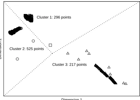
only 15 dimensions. A scatterplot of the programgzipprojected to 2 dimensions and clustered into
3 clusters using k-means is shown in Figure 5.
5.1.2 BAYESIANINFORMATIONCRITERION
To compare the different clusterings formed for different k, we use the Bayesian Information Crite-rion, or BIC (Schwarz, 1978), as a measure of the “goodness of fit” of a clustering to a data set. The BIC is an approximation of the probability of the clustering, given the data that has been clustered. Thus, the larger the BIC score, the higher the probability that the clustering being scored is a “good fit” to the data being clustered. The BIC formulation we use is appropriate for clustering with k-means, however other formulations of the BIC could also be used for other clustering models. The BIC is only one method of choosing a good model from a set of models; other methods such as the Akaike information criterion (AIC) (Akaike, 1974), minimum description length (MDL) (Rissanen, 1978), and Monte-carlo cross-validation (MCCV) (Smyth, 1996) may also be appropriate.
Dimension 2
Dimension 1 Cluster 1: 296 points
Cluster 2: 525 points
Cluster 3: 217 points
Figure 5: This plot shows a two-dimensional projection of the basic block vectors for the program
gzip, having 1038 total intervals, and clustered into three clusters with k-means. The
lines show divisions between the three clusters. Note that SimPoint normally operates in more than two dimensions, but this illustrates the fact that that program behavior does form natural groups that can be found through data clustering.
number of clusters). The BIC is formulated as
BIC(X,Ck) =
L
(X|Ck)−p
2log(n)
where
L
(X|Ck)is the log-likelihood of the clustered data X given the clustering Ckhaving k clusters,n=|X|is the number of points in the data, and p= (k−1) +dk+1=k(d+1)is the number of
parameters to estimate: (k−1)cluster probabilities, k cluster center estimates which each requires
d mean estimates, and one variance estimate (shared over all clusters). The log-likelihood of the k-means model given the data is
L
(X|Ck) = −nd2 log(2πσ
2)
−21σ2
k
∑
j=1i∑
∈Cj||Xi−cj||2+ k
∑
j=1njlog(nj/n)
where nj is the number of points in the jth cluster (so nj/n is the estimated prior probability of
cluster j), and σ2 is the average squared Euclidean distance from each point to its cluster center.
The term Cjrepresents the set of all indexes of X that are members of cluster j, Xiis the ith point in
data set X , and cj=nj1 ∑i∈CjXiis the location of the jth cluster center. The center cjis the maximum
likelihood solution for the cluster’s center. The maximum likelihood estimator forσ2is
ˆ
σ2 = 1
nd
k
∑
j=1i∑
∈CjFor the purposes of calculating the BIC, we can substitute this maximum likelihood estimate forσ2 into the log-likelihood formulation, to get a simpler version:
L
(X|Ck) = −nd2 log(2πσ
2)−nd
2 +
k
∑
j=1njlog(nj/n).
The BIC formulation we present basically follows that given by Pelleg and Moore (2000).
For a given program and inputs, the BIC score is calculated for each k-means clustering, for K in the range 1 to K. We then choose the clustering that achieves a BIC score that is close to the highest BIC score seen. This is explained more in Section 7.
5.2 Clusters and Phase Behavior
The bottom plots in Figures 1 and 2 show the results of running our phase-finding clustering
al-gorithm on gzipandgcc. These results use an interval length of 10 million instructions and the
maximum number of phases (K) is set to 10. The horizontal axis corresponds to the execution of the program (in billions of instructions), and each interval is classified to belong to one of the clusters (labeled on the vertical axis).
Forgzip, the program’s execution is partitioned into 4 clusters. Looking at the middle plot for
comparison, the cluster behavior captured by our algorithm lines up quite closely with the behavior of the program. Clusters 2 and 4 represent the large sections of execution which are similar to one another. Cluster 3 captures the smaller phase that lies in between these larger phases. Cluster 1 represents the phase transitions between the three dominant phases. The intervals in cluster 1 are grouped into the same phase because they execute a similar combination of code, which happens to be part of the code behavior in either cluster 2 or 4 and part of code executed in cluster 3. These transition points in cluster 1 also correspond to the same intervals that have large spikes in CPI seen in the top graph (these spikes are due to increased cache misses for those regions).
The bottom plot of Figure 2 shows how gccis partitioned into 8 clusters. Comparing this to
the middle and top plots in the same figure, we see that even the more complicated behavior ofgcc
is captured well by SimPoint. The dominant behaviors in the top two graphs can be seen grouped together in phases 1, 3, 5,and 7.
6. Choosing Simulation Points from the Phase Classification
After the phase classification algorithm has done its job, intervals with similar code usage will be grouped together into the same phases (clusters). Then from each phase, SimPoint chooses one representative interval that will be simulated in detail to represent the behavior of the whole phase. Therefore, by simulating only one representative interval per phase, we can extrapolate and capture the behavior of the entire program.
To choose a representative for a cluster, SimPoint picks the interval that is closest (Euclidean distance) to the cluster’s k-means center. The center can be viewed as a pseudo-interval which behaves most like the average behavior of the entire phase. Most likely there is no interval that exactly matches the center, so SimPoint chooses the closest interval. The selected interval is called a simulation point for that phase (Perelman et al., 2003; Sherwood et al., 2002). We can then perform detailed simulation on the set of simulation points.
the simulation point was taken divided by the number of instructions in the program. With the weights and the detailed simulation results of each simulation point, we can compute a weighted average for the architecture metric of interest (CPI, cache miss rate, etc.) for the entire program’s execution.
These simulation points are chosen once for a program/input combination because they are chosen based only on how the code is executed, and not based on architecture metrics. Therefore, they only need to be calculated once for a binary/input combination and can be used repeatedly across all of the runs for an architecture design space exploration.
The number of simulation points that SimPoint chooses has a direct effect on the simulation time that will be required for those points. The maximum number of clusters, K, along with the interval length, represents the maximum amount of simulation time that will be needed. When fixed
length intervals are used,(K∗interval length)is a limit on the number of simulated instructions.
SimPoint allows users to trade off simulation time with accuracy. Researchers in architecture tend to want to keep simulation time to below a fixed number of instructions (e.g., 300 million)
for a run. If this is a goal, we find that an interval length of 10 million instructions with K =30
provides very good accuracy (as we show in this paper) with reasonable simulation time (220 million instructions on average). If even more accuracy is desired, then decreasing the interval length to 1
million and setting K=300 performs well for the SPEC 2000 programs, as does setting K=√n
(where n is the number of clustered intervals). Empirically we discovered that as the granularity becomes finer, the number of phases discovered increases at a sub-linear rate. The upper bound defined by this square-root heuristic works well for the SPEC benchmarks.
The length of the interval chosen by users of SimPoint depends upon their simulation infras-tructure and how much they want to deal with warmup. Warmup is the process of initializing the simulator’s state (caches, branch predictor, etc.) at the start of a simulation point so that it is the same as if we simulated from the beginning of the program to that point. For many programs, using a long interval length (e.g., more than 100 million instructions) will make warmup unnecessary. This is the approach used by Intel’s PinPoint for simulation (Patil et al., 2004). They simulate intervals of length 300-500 million instructions so they do not have to worry about implementing warmup in their simulation infrastructure. With such long intervals the architecture structures are warmed up sufficiently during the beginning of the interval’s execution to provide accurate simulation results. In comparison, short interval lengths can be used, but this requires having an approach for warming up the architecture state. One way to do this is with an architecture checkpoint, which stores the po-tential contents of the major architecture components at the start of the simulation point (Biesbrouck et al., 2005). This can significantly reduce warmup time, since warmup consists of just reading the checkpoint from a file and using it to initialize the architecture structures.
6.1 Accuracy of SimPoint
We now show the accuracy of using SimPoint for the complete SPEC 2000 benchmark suite and their reference inputs. Figure 6 shows the simulation accuracy results using SimPoint (and other methods) for the SPEC 2000 programs when compared to the complete execution of the programs. For these results we use an interval length of 100 million instructions and limit the number of
simulation points to no more than 10. With the above parameters SimPoint finds 4 phases forgzip,
68% 51% 58% 13% 33% 23%
4% 8% 2% 8%
3736% 1986% 0% 10% 20% 30% 40% 50% 60% 70% 80% 90% 100%
gzip gcc Median Max
E rr o r in P e rf o rm a n c e E s ti m a ti o n ( IP C )
From Start Skip 1 Billion Sample Per Phase
Figure 6: Simulation accuracy for the SPEC 2000 benchmark suite when performing detailed simu-lation for several hundred million instructions compared to simulating the entire execution of the program. Results are shown for simulating from the start of the program’s execu-tion, for fast-forwarding 1 billion instructions before simulating, and for using SimPoint to choose at most ten 100-million-instruction intervals to simulate. The results are shown as percent error of predicted IPC, which is how much the estimated IPC using SimPoint is different from the complete execution of the program. IPC is the inverse of CPI. The median and maximum results are for the complete SPEC 2000 benchmarks.
that a total of 400 million instructions were simulated forgzip. The results show that this results in
only a 4% error in performance estimation forgzip.
For these results, we compare this estimated IPC using SimPoint to the baseline IPC. IPC (In-structions Per Cycle) is the inverse of CPI, and often used instead of CPI when describing perfor-mance. The baseline was gathered from spending months of simulation time to simulate the entire execution of each SPEC program. The results in Figure 6 compare SimPoint to how architecture re-searchers use to choose where to simulate before SimPoint. The first technique was to just simulate the first N million instructions of a benchmark’s execution. The second technique was to blindly skip the first billion instructions of execution to get past the initialization of the program’s execu-tion, and then simulate for N million instructions. The results show that simulating from the start of execution, for the exact same number of instructions as simulated with SimPoint, results in a median error of 58%. If instead, we fast forwarded for 1 billion instructions and then simulate for the same number of instructions as chosen by SimPoint, we see a median 23% IPC error. When using SimPoint to create multiple simulation points we have a median IPC error of 2%. Note that the maximum error seen for the prior techniques are significant for the SPEC programs, but it is very reasonable (only 8%) for SimPoint.
6.2 Relative Error During Design Space Exploration
gcc-166 0
0.5 1 1.5 2 2.5
1 2 3 4 5 6 7 8 9 10 11 12 13 14 15 16 17 18 19
C onfiguration
IP
C
0% 5% 10% 15% 20%
DL
1/
UL
2C
ac
he
MR
T rue IPC S P IPC
T rue DL1 S P DL1
T rue UL2 S P UL2
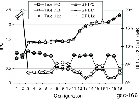
Figure 7: This plot shows the true and estimated IPC and cache miss rates for 19 different
architec-ture configurations for the programgcc. The left y-axis is for the IPC and the right y-axis
is for the cache miss rates for the L1 data cache and unified L2 cache. Results are shown for the complete execution of the configuration and when using SimPoint.
low error rate for a single configuration is not as important as achieving the same relative error rates across the design space search and having them all biased in the same direction.
We now examine how SimPoint tracks the relative change in hardware metrics across several different architecture configurations. To examine the independence of the simulation points from the underlying architecture, we used the simulation points for the SimPoint algorithm with an in-terval length of 1 million instructions and the maximum K set to 300. For the program/input runs examined, we performed full program simulations while varying the memory hierarchy, and for every run we used the same set of simulation points when calculating the SimPoint estimates. We varied the configurations and the latencies of the L1 and L2 caches as described by Perelman et al. (2003).
Figure 7 shows the results across 19 different architecture configurations forgcc-166. The left
y-axis represents the performance in Instructions Per Cycle (IPC) and the x-axis represents different memory configurations from the baseline architecture. The right y-axis shows the miss rates for the data cache and unified L2 cache, and the L2 miss rate is a local miss rate. For each metric, two lines are shown: “True” for the true metric from the complete detailed simulation, and the “SP” for the estimated metric using our simulation points. For the results, the configurations on the x-axis are sorted by the IPC of the full run.
program/input. This is true for both IPC and cache miss rates. We believe one reason for the bias is that SimPoint chooses the most representative interval from each phase, and intervals that represent phase change boundaries are less likely to be fully represented across the chosen simulation points.
7. Clustering Analysis
In this section we describe the primary parameters that have influence on how SimPoint and the k-means algorithm behave. We first focus on how we achieve a reasonable running time for k-k-means, and then examine how to search over k to find a good clustering. For the experiments in this section, we use basic block vectors with 100 million instruction intervals. Where it is not specified, we also
use k=30 clusters and 15 projected dimensions.
7.1 Methods for Reducing the Run-Time of k-Means
Even though SimPoint only needs to be run once per binary/input combination, we still want a fast clustering algorithm that produces accurate simulation points. To address the run-time of SimPoint, we first look at the three parts which affect most the running time of a single run of k-means. The three parts are the number of intervals to cluster, the dimension of the intervals being clustered, and the number of iterations it takes to perform a clustering.
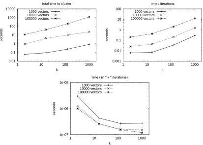
We first examine how the number of intervals affects the running time of the SimPoint algorithm. Figure 8 shows the time (in seconds) for running SimPoint on different numbers of intervals as we vary the number of clusters. For this experiment, the clustered vectors are randomly generated from uniformly random noise in 15 dimensions. We use random data in these experiments because it does not bias these results based on a particular benchmark and it gives comparable results across a wide range of parameter settings. But more importantly, prior theoretical work by Indyk et al. (1999) suggests that it is most difficult to accelerate (i.e. make more efficient using geometric reasoning) clustering algorithms on data without structure, such as uniformly random data. This is supported by experiments by Moore (2000) and Elkan (2003). So these experiments form a comparable set of challenging results for the per-iteration run-time of SimPoint. The number of iterations will vary depending on the structure of the data, however. For example, using k-means to cluster data from very well-separated clusters is likely to converge in a low number of iterations, while clusters which overlap are likely to require more iterations.
The first graph shows that for 100,000 vectors and k=128, it took about 3.5 minutes for
0.01 0.1 1 10 100 1000 10000
1 10 100 1000
seconds
k total time to cluster
1000 vectors 10000 vectors 100000 vectors
0.001 0.01 0.1 1 10 100
1 10 100 1000
seconds
k time / iterations
1000 vectors 10000 vectors 100000 vectors
1e-07 1e-06 1e-05
1 10 100 1000
seconds
k
time / (n * k * iterations)
1000 vectors 10000 vectors 100000 vectors
Figure 8: These plots show how varying the number of vectors and clusters affects the amount of time required to cluster with SimPoint 3.0. For this experiment we generated uniformly random data in 15 dimensions. The first plot shows total time, the second plot shows the time normalized by the number of iterations performed, and the third plot shows the time normalized by the number of basic operations performed. Both the number of vectors and the number of clusters have a linear influence on the run-time of k-means. The bottom plot shows a decreasing trend due to optimizations in k-means which are more beneficial for larger k.
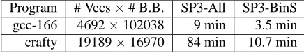
Program # Vecs×# B.B. SP3-All SP3-BinS gcc-166 4692×102038 9 min 3.5 min crafty 19189×16970 84 min 10.7 min
Table 4: This table shows the running times (in minutes) by SimPoint 3.0 without using binary search (SP3-All) and SimPoint 3.0 using binary search (SP3-BinS). SimPoint is run searching for the best clustering from k=1 to 100, uses 5 random seeds per k, and projects the vectors to 15 dimensions. The second column shows how many vectors and the size of the vector (static basic blocks) the programs have.
7.1.1 NUMBER OFINTERVALS ANDSUB-SAMPLING
Each iteration of the k-means algorithm has a run-time that is linear in the number of clusters, the number of intervals, and the dimensionality. However, since k-means is an iterative algorithm, many iterations may be required to reach convergence. We already found in prior work (Sherwood et al., 2002), and revisit in Section 7.1.2 that we can reduce the number of dimensions down to 15 and still maintain SimPoint’s accuracy. Therefore, the main influence on execution time for SimPoint is the number of intervals.
To show this effect, Table 4 shows the SimPoint running time for gcc-166 andcrafty-ref,
which shows the lower and upper limits for the number of intervals and basic block vectors seen in SPEC 2000 with an interval length of 10 million instructions. The second and third columns show the number of intervals and original number of dimensions for each basic block vector. The last two columns show the time it took to execute SimPoint 3.0 searching for the best clustering from k=1 to 100, with 5 random initializations (seeds) per k. The fourth column shows the time it took to run SimPoint when searching over all k, and the last column shows clustering time when using the new binary search described in Section 7.2.3. The results show that increasing the number of intervals by 4 times increased the running time of SimPoint around 10 times. The results also show that the number of intervals clustered has a large impact on the running time of SimPoint, since it
can take many iterations to converge, which is the case forcrafty. We used 15 dimensions during
clustering for these results.
The effect of the number of intervals on the running time of SimPoint becomes critical when using very small interval lengths like 1 million instructions or fewer, which can create millions of intervals to cluster. To speed the execution of SimPoint on these very large inputs, we sub-sample the set of intervals that will be clustered, and run k-means on only this sample. To sample with SimPoint, the user specifies the number of desired interval samples, and then SimPoint chooses that many intervals (without replacement). The probability of each interval being chosen is proportional to the weight of its interval (the number of dynamically executed instructions it represents). For vectors which all represent the same interval length (as we consider in this paper), this weight is uniform. If vectors represent non-uniform interval lengths (called variable-length intervals, or VLIs), then each vector’s weight is proportional to its interval length. We summarize our work with variable length intervals in Section 9.
intervals and assigns each interval to the cluster that has the nearest center (centroid) to that interval. This then represents the final clustering from which the simulation points are chosen. We originally examined using sub-sampling for variable length intervals (VLI) in Lau et al. (2005a). When us-ing VLIs we had millions of intervals, and had to sub-sample 10,000 to 100,000 intervals for the clustering to achieve a reasonable running time for SimPoint, while still providing very accurate simulation points.
The experiments shown in Figure 9 show the effects of sub-sampling across all the SPEC 2000 benchmarks using an interval length of 10 million instructions, 30 clusters, and 15 projected di-mensions. Results are shown for creating the initial clustering using sub-sampling with only 1/8, 1/4, 1/2, and all of the execution intervals in each program, as described above. The first two plots show the effects of sub-sampling on the CPI errors and k-means variance, both of which degrade gracefully when smaller samples are used. The average SPEC INT (integer) and SPEC FP (floating point) average results are shown. It is standard to break the results into these two groupings for architecture results. The CPI error is computed in the following manner:
CPI Error=|True CPI−SimPoint Estimated CPI|
True CPI .
The average k-means variance is the average squared distance between every frequency vector and its closest cluster center. Lower variances are better. When sub-sampling, we still report the variance based on every vector (not just the sub-sampled ones). The relative k-means variance reported in the experiments is measured on a per-input basis as the ratio of the k-means variance for clustering on a sample to that of clustering on the whole input.
As shown in the second graph of Figure 9, sub-sampling a program can cause k-means to find a slightly less representative clustering, which results in higher k-means variance on average. Note that the k-means variance for these experiments are reported on all the input vectors, not just the sampled ones. Even so, when sub-sampling, we found in some cases that it can reduce the k-means variance and/or CPI error (compared to using all the vectors), because sub-sampling can remove outliers in the data set that k-means may be trying to fit. This is a benefit noted in the work of Fayyad et al. (1998) when they use subsampling to initialize iterative clustering algorithms.
It is interesting to note the difference between floating point and integer programs, as shown in the first two plots. The results shown in the first plot show we can capture the behavior of the SPEC floating point programs more easily, that is, without using all the original data. In addition, the second plot suggests that SPEC floating point programs are also easier to cluster than the SPEC INT, as we can do quite well (in terms of k-means variance) even with only small samples. This suggests that they have more regular or uniform code usage patterns than integer programs. The third plot shows the effect of the number of vectors on the running time of SimPoint. This plot shows the time required to cluster all of the benchmark/input combinations and their 3 sub-sampled versions. In addition, we have fit a logarithmic curve with least-squares to the points to give a rough idea of the growth of the run-time. Note that two different data sets with the same number of vectors may require different amounts of time to cluster due to the number of k-means iterations required for the clustering to converge.
7.1.2 NUMBER OFDIMENSIONS ANDRANDOMPROJECTION
0.005 0.01 0.015 0.02 0.025 0.03 0.035
0.1 0.2 0.3 0.4 0.5 0.6 0.7 0.8 0.9 1
CPI error
sample fraction INT programs
FP programs
1 1.05 1.1 1.15 1.2 1.25 1.3 1.35
0.1 0.2 0.3 0.4 0.5 0.6 0.7 0.8 0.9 1
average relative k-means variance
sample fraction INT programs
FP programs
0 5 10 15 20 25 30 35 40
0 5 10 15 20 25 30 35 40 45
time (seconds)
number of vectors (sample size) x1000
Figure 9: These three plots show how sub-sampling before clustering affects the CPI errors, k-means variance, and the run-time of SimPoint. The first plot shows the average CPI error across the integer and floating-point SPEC benchmarks. The second plot shows the average k-means clustering variance relative to clustering with all the vectors. The last plot shows a scatter plot of the run-time to cluster the full benchmarks and sub-sampled versions, and a logarithmic curve fit with least squares.
jected dimensions on both the CPI error (left) and the run-time of SimPoint (right). For this exper-iment, we varied the number of projected dimensions from 1 to 100. As the number of dimensions increases, the time to cluster the vectors increases linearly, as expected. It is more interesting that the run-time also increases for very low dimensions. This is because the points are more “crowded” and the clusters are less well-separated, so k-means requires more iterations to converge.
0 0.01 0.02 0.03 0.04 0.05 0.06 0.07 0.08 0.09 0.1
0 10 20 30 40 50 60 70 80 90 100
CPI error
projected dimensions INT programs
FP programs
0.4 0.5 0.6 0.7 0.8 0.9 1
0 10 20 30 40 50 60 70 80 90 100
time (relative to 100 dimensions)
projected dimensions INT programs
FP programs
Figure 10: These two plots show the effects of changing the number of projected dimensions when using SimPoint. The default number of projected dimensions SimPoint uses is 15, but here we show results for 1 to 100 dimensions. The left plot shows the average CPI error, and the right plot shows the average time relative to 100 dimensions. Both plots are
averaged over all the SPEC 2000 benchmarks, for a fixed k=30 clusters.
to a poor solution, since the input space is not very densely filled. Therefore, it is wise to choose a dimension that is low enough to allow k-means to find a good clustering, but not so low that critical information is lost. We find that 15 dimensions works well in these regards.
7.1.3 NUMBER OFITERATIONSNEEDED
The final aspect we examine for affecting the running time of the k-means algorithm is the number of iterations it takes for a run to converge. We provide this analysis to illustrate typical requirements of running SimPoint on a set of benchmarks, and because finding a tight upper-bound on the number of iterations required by k-means is an open problem (Dasgupta, 2003), we must rely on evidence to show us what to expect.
The k-means algorithm iterates either until it hits a user-specified maximum number of itera-tions, or until it reaches convergence. In SimPoint, the default limit is 100 iteraitera-tions, but this can easily be changed. More iterations may be required, especially if the number of intervals is very large compared to the number of clusters. The interaction between the number of intervals and the
number of iterations required is the reason for the large SimPoint running time forcrafty-refin
Table 4.
For our results, we observed that only 1.1% of all runs on all SPEC 2000 benchmarks reach 100 iterations. This experiment was with 10-million instruction intervals, k=30, 15 dimensions, and with 10 random initializations of k-means. Figure 11 shows the number of iterations required for all runs in this experiment. Out of all of the SPEC program and input combinations run, only
0 20 40 60 80 100
Number of iterations
ammp-ref applu-ref apsi-ref art-110 art-470
bzip2-graphic
bzip2-program bzip2-source crafty-ref eon-cook eon-kajiya
eon-rushmeier
equake-ref facerec-ref fma3d-ref galgel-ref gap-ref gcc-166 gcc-200
gcc-expr
gcc-integrate
gcc-scilab
gzip-graphic
gzip-log
gzip-program gzip-random gzip-source lucas-ref mcf-ref mesa-ref mgrid-ref parser-ref
perlbmk-diffmail
perlbmk-makerand
perlbmk-perfect
perlbmk-splitmail
sixtrack-ref
swim-ref twolf-ref
vortex-one
vortex-three vortex-two
vpr-route
wupwise-ref
Figure 11: This plot shows the number of iterations required for 10 randomized initializations of each benchmark, with 10 million instruction length intervals, k = 30, and 15 dimensions. Note that only three program/inputs had a total of 5 runs that required more than the default limit of 100 iterations, and these all converge within 160 iterations or less.
7.2 Searching for a Small k with a Good Clustering
We suggest setting the maximum number of clusters K as appropriate for the maximum amount of simulation time a user will tolerate for a single simulation. SimPoint uses three techniques to search over the possible clusterings, which we describe here. The goal is to try to pick a small k so that the number of simulation points is also small, thereby reducing the simulation time required.
7.2.1 SETTING THEBIC PERCENTAGE
As we examine several clusterings and values of k, we need to have a method for choosing the best clustering. The Bayesian Information Criterion (BIC) (Pelleg and Moore, 2000) gives a score of the how well a clustering represents the data it clustered. However, we have observed that the BIC score often increases as the number of clusters increase. Thus choosing the clustering with the highest BIC score can lead to often selecting the clustering with the most clusters. Therefore, we look at the range of BIC scores, and select the score which attains some high percentage of this range. The SimPoint default BIC threshold is 90%. When the BIC rises and then levels off as k increases, this method chooses a clustering with the fewest clusters that is near the maximum BIC value. Choosing a lower BIC threshold would prefer fewer clusters, but at the risk of less accurate simulation.
Figure 12 shows the effect of changing the BIC threshold on both the CPI error (left) and the number of simulation points chosen (right). These experiments are for using binary search
(ex-plained in Section 7.2.3) with K=30, 15 dimensions, and 5 random seeds. BIC thresholds of 70%,
80%, 90% and 100% are examined. As the BIC threshold decreases, the average number of simu-lation points decreases, and similarly the average CPI error increases. At the 70% BIC threshold,