-PAL: An Active Learning Approach to the Multi-Objective
Optimization Problem
Marcela Zuluaga [email protected]
Department of Computer Science ETH Zurich
Zurich, Switzerland
Andreas Krause [email protected]
Department of Computer Science ETH Zurich
Zurich, Switzerland
Markus P¨uschel [email protected]
Department of Computer Science ETH Zurich
Zurich, Switzerland
Editor:Kevin Murphy
Abstract
In many fields one encounters the challenge of identifying out of a pool of possible designs those that simultaneously optimize multiple objectives. In many applications an exhaustive search for the Pareto-optimal set is infeasible. To address this challenge, we propose the
-Pareto Active Learning (-PAL) algorithm which adaptively samples the design space
to predict a set of Pareto-optimal solutions that cover the true Pareto front of the design space with some granularity regulated by a parameter. Key features of-PALinclude (1)
modeling the objectives as draws from a Gaussian process distribution to capture structure and accommodate noisy evaluation; (2) a method to carefully choose the next design to evaluate to maximize progress; and (3) the ability to control prediction accuracy and sam-pling cost. We provide theoretical bounds on-PAL’s sampling cost required to achieve a
desired accuracy. Further, we perform an experimental evaluation on three real-world data sets that demonstrate -PAL’s effectiveness; in comparison to the state-of-the-art active
learning algorithm PAL,-PAL reduces the amount of computations and the number of
samples from the design space required to meet the user’s desired level of accuracy. In addition, we show that-PALimproves significantly over a state-of-the-art multi-objective
optimization method, saving in most cases 30% to 70% evaluations to achieve the same accuracy.
Keywords: multi-objective optimization, active learning, pareto optimality, Bayesian optimization, design space exploration
1. Introduction
0 5 10 15 20 25 30 35 f1
0 5 10 15 20 25 30 35
f2
Pareto front
-accurate Pareto front
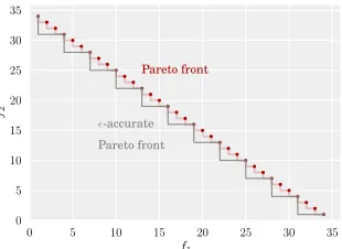
Figure 1: Assume that two objective functions are to be maximized simultaneously. This figure shows an example of the true Pareto front of a design space contrasted with an-accurate Pareto front, with = (3,3).
such as energy consumption, throughput, or chip area. Usually there is not a single design that excels in all objectives, and therefore one may be interested in identifying all (Pareto-)optimal designs. Furthermore, often in these domains, evaluating the objective functions is expensive and noisy. In hardware design, for example, synthesis of only one design can take hours or even days. The fundamental problem addressed in this paper is how to predict a Pareto-optimal set at low cost, i.e., by evaluating as few designs as possible.
In this paper we propose a solution for finite design spaces that we call the -Pareto Active Learning (-PAL) algorithm. The parameter allows users to control the accuracy
of the prediction produced by the algorithm. This accuracy is defined in terms of the density or granularity of the estimated Pareto front that is returned. Decreasing granularity means the algorithm can discard more points along its execution. Fewer Pareto points are returned, but spread to offer a wide range of trade-offs in the objective space.
More specifically, the granularity is controlled by a vector , containing one value per objective, which is given in the same units as the corresponding objective function. It specifies that for the user a difference ofin the objective space is negligible. Accordingly, an -accurate Pareto front might have fewer points than the true Pareto front. Fig. 1 visualizes this idea for two objective functions that are to be maximized simultaneously. The true Pareto-front is shown in red, and an-accurate Pareto front, which contains fewer points, is shown in grey. While the true Pareto front of a design space is unique, there can be many -accurate Pareto fronts; finding one of them efficiently is our goal.
-PAL has several key features. In the spirit of Bayesian optimization, it captures
domain knowledge about the regularity of the design space by using Gaussian process (GP) models to predict objective values for designs that have not been evaluated yet. Further, it uses the predictive uncertainty associated with these nonparametric models in order to guide the iterative sampling. Specifically, -PAL’s sampling strategy aims to maximize
progress on designs that are likely to be Pareto-optimal. -PAL iteratively discards points
that are either redundant or suboptimal, and it terminates when no more points can be removed in order to guarantee that, with high probability, the remaining points define an
A main contribution of this paper is the theoretical performance analysis of -PAL,
that provides bounds on the sampling cost required to achieve a desired accuracy. These bounds depend on the parameter and on the characteristics of the covariance function used for the GP models. Finally, we carry out an extensive empirical evaluation, where we demonstrate -PAL’s effectiveness on several real-world multi-objective optimization
problems. Two cases are from different applications in the domain of hardware design, in which it is very expensive to run low level synthesis to obtain the exact cost and performance of a single design (Zuluaga et al., 2012b; Almer et al., 2011). The third application is from software optimization, where different compilation settings are evaluated for performance and memory footprint size (Siegmund et al., 2012).
We compare the performance of -PAL against PAL, a predecessor of-PAL proposed
by Zuluaga et al. (2013), and with another state-of-the-art multi-objective optimization method called ParEGO, proposed by Knowles (2006). Across all data sets and almost all desired accuracies, -PAL outperforms ParEGO, requiring in most cases 30% to 70% less
function evaluations. In comparison to PAL, our experiments show that-PALreduces the
runtime by one to two orders of magnitude, while also reducing the number of evaluations and offering more flexibility in the desired error.
1.1 Main Contributions
Our main contributions are summarized as follows.
• We propose -PAL, an active learning approach towards identifying a set of optimal
solutions in a given multi-objective optimization problem in which function evalua-tions are expensive. This includes sampling strategy and stopping criteria. -PAL
allows users to specify the desired level of granularity through the parameter , and guarantees that with high probability an-accurate Pareto front is returned.
• We theoretically analyze-PALwhen the design space is a finite set, and the objective
functions satisfy regularity assumptions as specified via a positive definite kernel. We provide bounds on the number of iterations required by the algorithm to achieve a desired target accuracy.
• In comparison to the state-of-the-art algorithm PAL, -PAL reduces the asymptotic
complexity of the number of computations performed in each iteration, making it more suitable for larger design spaces.
• We perform an extensive experimental evaluation to demonstrate -PAL’s
effective-ness and superiority over PAL and ParEGO on three real-world multi-objective opti-mization problems.
1.2 Organization
In Section 2, we introduce background concepts such as multi-objective optimization, Pareto optimality,-accurate Pareto optimality, and Gaussian processes. In addition, we formally define the problem tackled in this paper. Section 3 presents the proposed algorithm
Section 4, we present the theoretical analysis of the algorithm and provide upper bounds for the number of samples needed before -PAL terminates, when the target functions
have bounded RKHS norm. Section 5 discusses some implementation issues that might arise in practice when using our algorithm. Section 6 reviews related work in the areas of multi-objective optimization, Bayesian optimization and evolutionary algorithms. Section 7 shows the effectiveness of-PALin comparison with state-of-the-art alternative algorithms,
using three data sets obtained from real applications. In the Appendix, we prove our main Theorem, which is stated in Section 4.
2. Background and Problem Statement
In this section, we review multi-objective optimization and Pareto optimality, and introduce the terminology and notation used in the rest of the paper. At the end of the section, we formally define the problem addresses by -PAL.
2.1 Multi-Objective Optimization
We consider a multi-objective optimization problem over a finite set E (called the de-sign space). This means that we wish to simultaneously optimize m objective functions
f1, . . . , fm : E → R. In our analysis, we assume that f1(x), . . . , fm(x) are to be
maxi-mized, however our results straightforwardly generalize to a minimization or a combined minimization/maximization problem. We use the notation f(x) = (f1(x), . . . , fm(x)) to
refer to the vector of all objectives evaluated on the input x. The objective space is the imagef(E)⊂Rm.1
2.2 Pareto Optimality
The goal in multi-objective optimization is to identify2 the Pareto set of E. Formally, we consider the canonical partial order in Rm: y y0 iff yi ≥ yi0, 1 ≤i ≤m, and define the
induced relation on E: xx0 iff f(x)f(x0). We say that xdominates x0 in this case.
Note that on E is not a partial order, but only a preorder, since it lacks antisymmetry (i.e., two different designs can have the same objectives).
Definition 1 (Pareto set) The Pareto set Π(f(E))) in the objective space f(E) ⊂ Rm
is, as usual, the set of maximal points. Further, we call any set Π(E)⊆E a Pareto set of
E if it satisfies
f(Π(E)) = Π(f(E))).
In words, Π(E) is any set of designs that yields all optimal objectives. It is not unique since
on E is not antisymmetric.
1. Scalars and functions that return scalars are written unbolded; tuples and vectors are boldfaced. 2. Note that one may also approach multi-objective optimization via scalarization, see, e.g., Roijers et al.
(c)
(a) (b)
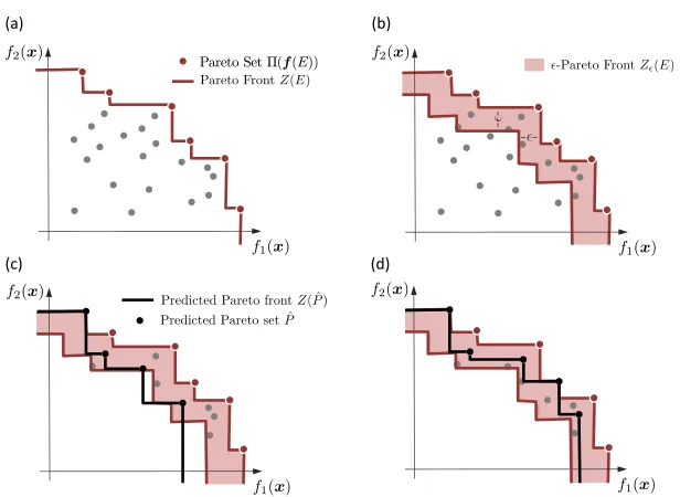
(d) Pareto Set ¦(f(E))
Figure 2: (a) Example of Pareto set and Pareto front form= 2. (b) Example of an-Pareto front form= 2. (c) Example of a predicted Pareto set that is not-accurate. (d) Example of a predicted Pareto set that is-accurate.
Definition 2 (Pareto front) We define the Pareto frontZ(E) as the set of points inRm
that constitutes the surface of the space dominated by the Pareto setΠ(f(E)). Formally,
Z(E) = ∂{y∈Rm : there is an x∈E with f(x)y)}. (1)
Hereby, the operator∂ applied to a set Y denotes the boundary of Y.
Fig. 2(a) visualizes the concepts of Pareto set and Pareto front for m= 2.
2.3 -Pareto Optimality
We now relax the relation in Rm and E for the purpose of our algorithm by adding a
small tolerance. Consider a vector = (1, . . . , d), with i ≥ 0, 1 ≤ i≤ m. We say that
a point y∈ Rm -dominates y0, written as y y0, if y+ y0. As before, we pull the
relation to E: x x0 iff f(x) f(x0). Note that this relation is neither a partial order
nor a preorder: antiysmmetry and transitivity do not hold.
We use this relation next to define an appropriate notion of -accurate Pareto set. To do so we first need two auxiliary definitions.
Definition 3 (-Pareto front) We define the -Pareto front Z(E) of E as the set of
points between Z(E) and Z(E)−, including the boundaries. Formally,
Z(E) ={y∈Rm :y0 y for some y0∈Z(E) and y y00 for some y00∈Z(E)}
Definition 4 (-Pareto front covering) We say that a nonempty setC ⊆Z(E) covers Z(E), if for every pointy∈Z(E) there is at least one point y0 ∈C s.t. y0 y.
In words, Definition 4 requires that the Pareto front spanned by Π(C) is contained inZ(E).
Definition 5 (-Accurate Pareto set) We call a set of points Π(E)⊆E an-accurate
Pareto set ofE, if f(Π(E)) coversZ(E).
In words, for an -accurate Pareto set, the associated front is contained in the -Pareto frontZ(E) and it contains no suboptimal designs. As examples, the set with objectives ˆP
in Fig. 2(c) does not satisfy this property, but in Fig. 2(d) it does. Note that the-accurate Pareto set may have fewer points than the actual Pareto set.
An -accurate Pareto set Π(E) is a natural approximate substitute of the original set E. Having access to it, one can rest assured that for any point on the Pareto front Z(E) associated with E, there is some element x ∈ Π(E) which is at most worse according
to all of the objectives. The high level goal of our algorithm -PAL is to find, with few
evaluationsf(x), a small -accurate Pareto set of E.
2.4 Gaussian Processes (GP)
-PAL models f as a draw from anm-variate Gaussian process (GP) distribution. A GP
distribution over a real function f(x) is fully specified by its mean function µ(x) and its covariance function k(x,x0) (Rasmussen and Williams, 2006). The kernel or covariance
function k captures regularity in the form of the correlation of the marginal distributions
f(x) and f(x0).
In our multi-objective setting, we model each objective function fi(x) as a draw from
an independent3 GP distribution.
On every iterationt in our algorithm we choose a design xt to evaluate, which yields a
noisy sample4 y
t,i =fi(xt) +νt,i; afterT iterations we have a vector yT ,i = (y1,i, . . . , yT,i).
Assumingνt,i∼N(0, σ2) (i.i.d. Gaussian noise), the posterior distribution offiis a Gaussian
process with meanµT ,i(x), covariance kT ,i(x,x0), and variance σT ,i2 (x):
µT ,i(x) =kT ,i(x)T(KT ,i+σ2I)−1yT ,i, (2)
kT ,i(x,x0) =ki(x,x0)−kT ,i(x)T(KT ,i+σ2I)−1kT ,i(x0), (3)
σT ,i2 (x) =kT ,i(x,x), (4)
wherex,x0 ∈E,kT ,i(x) = (ki(x,xt))1≤t≤T and KT ,i = (ki(xj,x`))1≤j,`≤T. Note that this
posterior distribution captures our uncertainty aboutf(x) for all pointsx∈E.
2.5 Reproducing Kernel Hilbert Spaces (RKHS)
Using Gaussian processes to model the target functionsfi assumes that we know the prior
from which they have been generated. This is rarely the case in practice. Therefore, for
our theoretical analysis we take a more agnostic approach in which we assume that fi are
arbitrary functions from the RKHS associated with kernelk.
The RKHSHk(E) is a Hilbert space consisting of functionsf on the domainE, endowed
with an inner producth·,·ikthat satisfies the following properties with respect to a positive
definite functionk:
• For every x∈E,k(x,x0) as a function ofx0 belongs to Hk(E).
• The reproducing property holds fork, i.e., hf, k(x,·)ik=f(x).
The smoothness of the functions f ∈ Hk(E) with respect to k is encoded by the norm
||f||k =
p
hf, fik. Functions with low norm are usually relatively smooth. In our case, as E is a finite set, anyf is guaranteed to have bounded norm, i.e.,||f||k<∞, as long as the
kernel is universal (such as the Gaussian kernel).
2.6 Problem Statement
LetE be a finite set with a positive definite kernel. We wish to simultaneously optimize m
objective functions f1, . . . , fm :E →R, considering that evaluating f(x) for anyx∈E is
expensive. We wish to identify an -accurate Pareto set Π(E) ⊆E while minimizing the
number of evaluationsf(x).
In the following, we develop an active learning algorithm that iteratively and adaptively selects a sequence of designs x1,x2, . . . to be evaluated, and that uses these evaluations along with the model’s predictive uncertainty to predict an-accurate Pareto set ofE. This iterative algorithm terminates when, with high probability, an -accurate Pareto set of E
has been found, and therefore no more evaluations are needed. In addition, we theoretically analyze our algorithm and provide a bound on the number of evaluations required by the algorithm to generate an -accurate prediction.
3. -PAL Algorithm
In this section we describe our algorithm: -Pareto Active Learning (-PAL).
3.1 Overview
Our approach to predicting an -accurate Pareto set of E trains GP models on a small subset of E. The models predict the objective functions fi, 1 ≤ i ≤ m, allowing us to
make statistical inferences about the Pareto-optimality of every point inE. The true value of f(x) is approximated by the models as ˆf(x) = µ(x) = (µi(x))16i6m. Additionally σ(x) = (σi(x))16i6m is interpreted as the uncertainty of this prediction. We capture this
uncertainty through the hyper-rectangle5
Qµ,σ,β(x)={y:µ(x)−β1/2σ(x)yµ(x)+β1/2σ(x)}, (5)
whereβ is a scaling parameter to be chosen later.
The goal of the algorithm is to return a set ˆP ⊆ E such that, with high probability, ˆ
P is an -accurate Pareto set of E. ˆP may contain points that are not sampled yet, but
probabilistically, it is guaranteed to coverZ(E), i.e., with high probability, all points inE
are-dominated by a point in ˆP.
-PAL iterates over four stages: modeling, discarding, -Pareto front covering, and
sampling. It stops when all remaining points have been either sampled, discarded or de-termined to belong to Z(E) with high probability. The following sections explain each of
these stages, and Alg. 1 presents the corresponding pseudocode.
The algorithm maintains two working sets, indexed by the iteration number t, starting at 0:
• Ut: undecided points, U0 =E,
• Pt: points predicted to be members of an-accurate Pareto set of E,P0=∅.
On the first iteration (t= 0), all points inE are copied to a set U0. Subsequently, on any iteration t, a point to be sampled is chosen from Ut or Pt. Points in Ut that with high
probability are -dominated by another point are discarded, i.e., removed from Ut, and
points that are determined to belong toZ(E) are moved fromUtto setPt. The algorithm
terminates at some iteration T when UT is empty. Then ˆP = PT is returned. -PAL
guarantees that with high probability ˆP is an-accurate Pareto set ofE.
3.2 Modeling
-PAL uses Gaussian process inference to predict the mean vectorµt(x) and the standard
deviation vectorσt(x) of any pointx∈E that has not been discarded yet. This prediction
is generated based on the noisy samples obtained. Each pointx∈Pt∪Ut is then assigned
its uncertainty region, which is the hyperrectangle
Rt(x) =Rt−1(x)∩Qµt,σt,βt+1(x), (6)
where βt+1 is a positive value that defines how large this region is in proportion to σt. In Section 4 we will suggest a value for this parameter. The iterative intersection ensures that all uncertainty regions are non-increasing witht. Intuitively, for a pointx∈E that has not been evaluated yet, we can say that with high probability f(x)∈Rt(x).
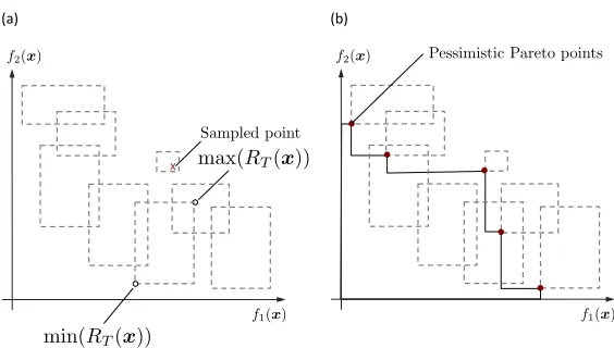
WithinRt(x), the pessimistic and optimistic outcomes are min(Rt(x)) and max(Rt(x)),
respectively, both taken in the partial order and unique. Fig. 3(a) shows this with an example. Notice that points that have been evaluated also have an uncertainty region, since we only have access to noisy samples on those points.
3.3 Discarding
The goal of this stage is to discard points inUt that with high probability are-dominated
by another point inE, while making sure that at least one of such dominating points ends up in PT.
Under uncertainty, a point xis-dominated by another pointx0, with high probability,
if the pessimistic outcome of x0 (min(Rt(x0))) -dominates the optimistic outcome of x
(max(Rt(x))):
max(Rt(x))min(Rt(x0)).
f1(x) f2(x)
d max(RT(x))
min(RT(x))
d max(RT(x))
min(RT(x))
Sampled point
f1(x)
f2(x) Pessimistic Pareto points
(a)$ (b)$
x$
Figure 3: (a) Example of min(Rt(x)) and max(Rt(x)) for m= 2. (b) Example of a set of
pessimistic Pareto points form= 2.
If this relationship does not hold, either the uncertainty regions are still too large to draw any conclusions, or xand x0 are not comparable.
To check if a point is-dominated by another one inE,-PALcompares its relationship
with allpessimistic Pareto points.
Definition 6 (Pessimistic Pareto set) For a subset D⊆E, we define ppess(D), or the
pessimistic Pareto set of D, as the set of points x ∈ D for which there is no other point
x0 ∈D such that
min(Rt(x))min(Rt(x0)).
Fig. 3(b) illustrates this situation.
We discard any pointx∈Ut\ppess(Pt∪Ut) ifxx0 for somex0 ∈ppess(Pt∪Ut). This
ensures that no element inppess(St∪Pt∪Ut) is discarded and therefore, for every point that
is discarded there will always be a point in the working sets that -dominates it.
A point in ppess(Pt∪Ut) is only discarded if it is-dominated by any point in Pt, since
all points in Pt are already guaranteed to belong to the returned set ˆP. Points in Pt are
never discarded.
3.4 -Pareto Front Covering
The goal of -PAL is to empty Ut as fast as possible, i.e., with the least amount of points
sampled and with the least amount of points in Pt needed to cover the -Pareto front of E. As previously stated, a point is moved to Pt if it can be determined that with high
probability it belongs to Z(E).
Therefore, care must be taken not to sample when all points inUtcan be either discarded
Definition 7 (x belongs to Z(E) with high probability) We can determine that with
high probability x∈E belongs toZ(E) if there is no other pointx0 ∈Pt∪Ut such that
max(Rt(x0))min(Rt(x)).
In this stage we attempt to update the set Pt, to make progress in covering the -Pareto
front of E, until we find a point inUt that cannot be moved toPt. After a point is moved
to Pt, we check what points in Ut are -dominated by it, and therefore can be discarded.
Details on this procedure can be found in Alg. 1.
3.5 Sampling
As long as Ut 6= ∅, on each iteration, a new point xt is selected for sampling with the
following selection rule. Each pointx∈Ut∪Pt is assigned a value
wt(x) = max
y,y0∈R
t(x)||
y−y0||2,
which is the diameter of its uncertainty regionRt(x). Amongst these points, the one with
the largestwt(x) (i.e., most uncertain) is chosen as the next samplextto be evaluated. We
refer towt(xt) aswt. Note that our approach does not simply pick the most uncertain point
over the whole spaceE, but only over the setUt∪Pt, i.e., the points that (in a statistically
plausible manner) might be useful in constructing an -accurate Pareto set. This is similar to exploration–exploitation tradeoffs commonly encountered in Bayesian optimization.
3.6 Stopping Criteria
The iterations terminate att=T when UT =∅, i.e., all points have been either moved to PT or have been discarded. The predicted set ˆP =PT is guaranteed to be an -accurate
Pareto set of E. Termination occurs at the latest when wt ≤ . In this case, dominated
points can be discarded in one pass.
3.7 Analysis of Execution Time
In this section, we review the most time consuming subroutines of -PAL and analyze
their computational cost, which depends on the number of points in the working sets:
nt =|Ut|+|Pt|. While n0 =|E| in the first iteration, discarded points are removed from the working sets and thus the number of computations is reduced as t increases. As it is not possible to make conclusions in how nt decreases with t, we assume the upper bound n=|E|. In practice, the number of computations is much lower for most iterations of the algorithm. On the other hand, we assume that the number m of objective functions is a small constant.
In the modeling stage, -PAL updates Gaussian process models and evaluates the
pre-diction µ and the uncertaintyσ for every point. Let s be the number of points that have been sampled, the complexity of this step isO(s3+ns2) (Rasmussen and Williams, 2006). Note that typically sn.
In the discarding stage, -PAL first finds the Pareto pessimistic points of a set. The
Algorithm 1 The-PALalgorithm
Input: design spaceE (|E|=n); GP priorµ0,i, σ0, kifor all 1≤i≤n;;βtfort∈N
Output: predicted Pareto set ˆP
1: P0=∅ {predicted set},U0=E{undecided set}
2: R0(x) =Rnfor allx∈E,t= 1
3: repeat
4: Pt=Pt−1, Ut=Ut−1
5: Modeling
6: Obtainµt(x) andσt(x) for allx∈Pt∪Ut
7: Rt(x) =Rt−1(x)∩Qµt,σt,βt+1(x) for allx∈Pt∪Ut
8: Discard
9: ppess(Pt) = Pareto pessimistic set ofPt
10: discard pointsxinUtthat are-dominated by some pointx0 inppess(Pt), i.e., where max(Rt(x))
min(Rt(x0)) (See Alg. 2 form= 2)
11: ppess(Pt∪Ut) = Pareto pessimistic set ofPt andUt
12: discard pointsxinUt\ppess(Pt∪Ut) that are-dominated by some pointx0 inppess(Pt∪Ut), i.e., where max(Rt(x))min(Rt(x0)). (See Alg. 2 form= 2)
13: -Pareto Front Covering
14: repeat
15: Choosex0= arg maxx∈Ut{wt(x)}
16: if for allx∈Pt∪Ut\ {x0}it holds that max(Rt(x))min(Rt(x0)) then 17: Pt=Pt∪ {x0},Ut=Ut\ {x0}
18: else
19: break
20: end if
21: untilUt=∅
22: Sampling
23: Choosext= arg maxx∈Ut∪Pt{wt(x)} 24: Sampleyt(xt) =f(xt) +νt
25: t=t+ 1
26: untilUt=∅
27: return Pˆ=Pt
Algorithm 2 Discard points inU that are -dominated byppess form= 2.
Input: setU; Pareto pessimistic setppess;
Output: updated setU
1: U0 ={(x,min(Rt(x)) +) :x∈ppess} ∪ {(x,max(Rt(x))) :x∈U\ppess} {U0 is a set of (x,( ˆf1,fˆ2))
pairs}
2: sortU = sortU0with respect to ˆf
1 in ascending order
3: currentM ax=−∞ 4: for(x,( ˆf1,fˆ2)) insortU do
5: if x∈ppess then
6: currentM ax= ˆf2
7: else
8: if fˆ2≤currentM axthen
9: U=U\ {x} {discardx}
10: end if
11: end if
12: end for
off2 seen so far. This procedure exhibits computational complexity ofO(nlogn) form= 2. The same computational complexity is achieved by a similar implementation for m = 3.
For m > 3, Kung et al. (1975) presents a divide and conquer algorithm with worst case
asymptotic complexity ofO(n(logn)m−2) +O(nlogn).
In the discarding stage, -PAL also discards points in a set U that are -dominated
by a set ppess. This means that, if done naively, every point max(x) with x ∈U must be compared with every min(x0) + with x0 ∈p
pess. However, this can be done by adapting the above mentioned implementations to compute the Pareto points of a set of vectors to substantially reduce the runtime of the algorithm. Alg. 2 shows the pseudocode for this adaptation. A joined setU0 is created from points max(x) withx∈U and min(x0) +with x0 ∈ppess. This joint list is ordered with respect to the first dimension f1. Then, the list is traversed in ascending order, but the maximum value of f2 is only updated by a point that belongs to ppess, and only points that belong to U can be discarded. For m ≥ 3 the adaptation of the algorithm by Kung et al. (1975) is analogous.
In the -Pareto front covering stage, -PAL checks if a point x can be guaranteed to
belong toZ(E) according to Definition 7. This is done by comparingxwith the rest of the
pointsx0 in the working sets, until a case in which min(Rt(x0)) +max(Rt(x)) is found.
The number of computations for this step isO(n); in practice, however, it is much smaller thann for most iterations. This operation might be done several times per iteration, until no more points inUt can be moved toPt orUt=∅. The number of times is assumed to be
much smaller thann.
The computational complexity of an iteration is therefore dependent on m and s. For
m= 2 andm= 3 it isO(ns2+s3+nlogn), and for m >3 it isO(n(logn)m−2) +O(ns2+
s3+nlogn).
4. Correctness and Sample Complexity
So far we have left the parameter βt undefined. In this section, we will choose a βt that
guarantees the correctness of the algorithm, and the number of iterations required to meet our bounds.
Of key importance in the convergence analysis is the effect of the regularity imposed by the kernel functionk. In our analysis, this effect is quantified by themaximum information gain associated with the GP prior. Formally, we consider the information gain
I(y1. . .yT;f) =H(f)−H(f |y1. . .yT),
i.e, the reduction of uncertainty on f caused by (noisy) observations of f on the T first sampled points. The crucial quantity governing the convergence rate is
γT = max y1...yT
I(y1. . .yT;f),
i.e., the maximal reduction of uncertainty achievable by sampling T points. Intuitively, if the kernel k imposes strong regularity (smoothness) on f, few samples suffice to gather much information about f, and as a consequence γT grows sub-linearly (exhibits a strong
key quantity in bounding the regret in single-objective GP optimization. Here, we show that this quantity more broadly governs convergence in the much more general problem of predicting the Pareto-optimal set in multi-criterion optimization.
We obtain bounds on the number of iterations required when assuming that the target functions fi, 0 ≤ i ≤ m, lie in the RKHS Hk(E) corresponding to kernel k(x,x0), and
that the noise νt is an arbitrary martingale difference sequence which has zero mean and
is uniformly bounded byσ. Furthermore, in order to obtain the bounds, it is necessary to specify an upper bound6 B on all||f
i||k.
The following theorem constitutes our main theoretical result.
Theorem 1 Assume that the true functions fi lie in the RKHS Hk(E) corresponding to
kernel k(x,x0), and that the noise νt has zero mean conditioned on the history and is
bounded by σ almost surely. Let δ ∈ (0,1) and ||fi||2k ≤ B. Running -PAL with βt =
2B2 + 300γ
tlog3(m|E|t/δ), prior GP(0, k(x,x0)) and noise N(0, σ2), the following holds
with probability1−δ.
An -accurate Pareto set can be obtained after at most T iterations, where T is the smallest number satisfying
r
C1βTγT
T ≥. (7)
Here, C1= 8/log(1 +σ−2), =||||∞, andγT depends on the type of kernel used.
This means that, with high probability,wtis bounded byO∗((B√γT+γT)/
√
T). Note that in practice one might want to, in addition to identifying an -accurate Pareto front, seek to be sufficiently confident such that for all predicted Pareto points (i.e., points x in PT
in Algorithm 1) it holds that wT(x) ≤ . This requirement can be added to the stopping
condition in Line 26 of Algorithm 1, and the same sample complexity of Theorem 1 holds.
4.1 Proof Outline
The above theorem implies that by specifyingδ and a target accuracy,-PAL
automati-cally stops when the target error is achieved with confidence 1−δ. Additionally, the theorem bounds the number of iterationsT required to obtain this result.
Our strategy for the proof consists of four parts. First, Lemma 1 shows that |fi(x)− µt−1,i(x)| ≤βt1/2σt−1,i(x) for 1 ≤i≤m,t ≥1, and for all x∈E. Then, we analyze how wt decreases with t. Subsequently, we relate and wt to ensure the termination of the
algorithm. The last two parts are analyzed in Section 4.2. Finally, Lemma 8 supports the accuracy of the -PAL, given that the proper βt value is used on every iterationt.
4.2 Reduction in Uncertainty
The first step of the proof is to show that with probability at least 1−δ,f(x) lies for all
x∈E within the uncertainty region (see (5) and (6)):
Rt(x) =Qµ0,σ0,β1(x)∩ · · · ∩Qµt,σt,βt+1(x),
which is achieved by choosingβt= 2B2+ 300γtlog3(m|E|t/δ).
Srinivas et al. (2010) showed that information gain can be expressed in terms of the pre-dicted variances. Similarly, we show how the cumulative Pt
k=1wk can also be expressed in
terms of maximum information gainγt. Since the sampling rules used by -PALguarantee
thatwtdecreases with t, we get the following bound forwt. With probability ≥1−δ,
wt≤
r
C1βtγt
t for all t≥1, (8)
whereC1 = 8/log(1 +σ−2) andβtis as before.
The proof is supported by Lemmas 1 to 5 found in the appendix of this paper. Key challenges and differences in comparison to Srinivas et al. (2010) include (1) dealing with multiple objectives; (2) the use of a different sampling criterion; and (3) incorporating the monotonic classification scheme.
We also show that, with probability 1−δ, the algorithm terminates with no further sampling at iteration T if
wT ≤, (9)
where=||||∞= max(i)1≤i≤m. This is proved in Lemma 7.
4.3 Explicit Bounds for the Squared Exponential Kernel
Theorem 1 holds for general covariance functions k(x,x0). Srinivas et al. (2010) derived
bounds forγT depending on the choice of kernel. These can be used to specialize Theorem 1.
We illustrate this using the squared exponential kernel as example, i.e., k(x,x0) = exp l−2kx−x0k2
2
for somel >0.
Let E ⊂ Rd be compact and convex, d ∈ N. According to Srinivas et al. (2010), for m= 1, there exists a constantK such that
γt≤Klogd+1tfor all t >1.
Form >1, since we assume i.i.d. GPs, we thus get
γt≤Kmlogd+1t
and hence the following corollary to Theorem 1.
Corollary 1 Let ki be the squared exponential kernel used by -PAL, and assume fi lies
in the RKHS with its norm bounded by ||fi||2k ≤ B, for all 1 ≤ i ≤ m. When choosing δ∈(0,1), a target accuracy specified by, the following holds with probability 1−δ. -PAL
terminates after at most T iterations, where T is the smallest number satisfying
q
16B2K2mlogd+1T + 2400K2m2log2(d+1)Tlog3(m|E|T /δ)
p
Tlog(1 +σ−2) ≥.
These results suggests that, under both scenarios,increases asT decreases in the following manner: Asymptotically, for any ρ >0, as well as fixedm,nand d, we have T =O( 1
5. Discussion and Implementation Details
We now discuss some of the limitations, choices made, and other aspects that arose when implementing and using our-PAL algorithm.
5.1 Sampling Strategy
After clearly non-competitive designs are removed in the discarding phase, our sampling strategy (Section 3.5) chooses the one with the highest uncertainty. Other choices would be possible, e.g, chosing the one that maximizes the expected gain in hypervolume. Our choice aims at reducing time to termination, which is achieved by reducing uncertainty in the model as fast as possible.
5.2 Parameterization
For practical usage, two parameters, namelyandδ, need to be specified. These parameters relate to the desired level of accuracy of the prediction. Our theoretical bounds are likely to be loose in practice; thus, it may be useful to choose more “aggressive” values than recommended by the theory. The choice of δ impacts the value of βt and therefore the
convergence rate of the algorithm, since the latter scales the uncertainty regions Rt(x).
Since the analysis is conservative, scaling down βt, possibly to be constant, is a viable
option.
In contrast, the choice of should pose no problem. One only may consider scaling the objective functions so that alli components of have comparable values.
5.3 Kernel Hyper-Parameters
So far, we have assumed that the kernel function is given. Usually, its parameters need to be chosen. Therefore, prior to running -PAL, it may be practical to randomly sample
a small fraction of the design space and to optimize the parameters (e.g., by maximizing the marginal likelihood). One may also consider maintaining uncertainty in the hyper-parameters by placing and updating priors on them. These can then be marginalized to obtain suitable hyper-rectangles to capture the uncertainty about the designs. This extension poses new challenges in computational efficiency (i.e., using approximate Bayesian inference), and we defer it to future work.
5.4 Scalability
5.5 Continuous vs. discrete domains
In our approach, we have focused on finite, discrete domainsE, which often naturally arise in design-space exploration problems as those considered in our experiments. For Lipschitz-continuous objectives (which are commonly assumed in Bayesian optimization), it is be possible to handle continuous compact domainsE via standard covering arguments. Given the allowed tolerancesand Lipschitz constants, one can construct a discretization ˆE such that for any point x∈E in the domain, there is one in the discretizationx0∈Eˆ such that f(x0) f(x). It can be seen that any-accurate Pareto set of ˆE is a 2-accurate Pareto
set of E. This discretization-based approach becomes impractical with higher dimensions. Developing a variant of our approach that does not require an explicit discretization is an interesting direction for future work.
5.6 Current Implementation
For our experimental evaluation, we implemented a prototype that is restricted to m = 2 objectives. The code is available at Zuluaga et al. (2015).
6. Related Work
We now discuss different lines of related work.
6.1 Evolutionary Algorithms
One class of approaches uses evolutionary algorithms to approximate the Pareto frontier via a population of evaluated designs that is iteratively evolved (K¨unzli et al., 2005; Coello et al., 2006; Zitzler et al., 2002). Most of these approaches do not use models for the objectives, and consequently cannot make predictions about unevaluated designs. As a consequence, a large number of evaluations are typically needed for convergence with reasonable accuracy. To overcome this challenge, model-based (or “response surface”) approaches approximate the objectives by models, which are fast to evaluate. A concrete example is the algorithm presented by Emmerich et al. (2006), which uses Gaussian random fields metamodels to predict the objective functions. These models are used to screen each generation of the population and to extract promising individuals. On the other hand, Laumanns and Oce-nasek (2002) and Buche et al. (2005) investigate the use of Gaussian models to maintain and improve the diversity of the population during the offspring-generation phase.
We will compare against ParEGO (Knowles, 2006) (explained in Section 6.6 below), which improves on the above work by combining the evolutionary approach with optimiza-tion to reduce the number of evaluaoptimiza-tions needed.
6.2 Scalarization to the Single-Objective Setting
optimizes simultaneously several single-objective subproblems that are created using differ-ent scalarization criteria. The diversity amongst the subproblems will lead to diversity in the approximated Pareto front.
A number of global optimization algorithms are also conditioned to the multi-objective setting by using scalarization. As a concrete example, Zhang et al. (2010) and Knowles (2006) extend the single-objective efficient global optimization (EGO) approach of Jones et al. (1998) by decomposing the optimization problem into several single-objective sub-problems. A GP model is built for every subproblem, and sample candidates are selected based on their expected improvement.
A major disadvantage of the scalarization approach is that without further assumptions (e.g., convexity) on the objectives, not all Pareto-optimal solutions can be recovered (Boyd and Vandenberghe, 2004). Therefore, we avoid scalarization in our approach.
6.3 Heuristics-based Methods
Instead of weighted combinations, numerous domain-specific heuristics have been proposed that aim at identifying Pareto-optimal solutions. These approaches typically combine search algorithms to suit the nature of the problem (Deng et al., 2008; Palermo et al., 2009; Zuluaga et al., 2012a) and defy theoretical analysis to provide bounds on the sampling cost. With this work we aim at creating a method that generalizes across a large range of applications and target scenarios and that is analyzable, i.e., comes with theoretical guarantees.
6.4 Single-Objective Bayesian Optimization and Active Learning
In the single-objective setting, there has been much work on active learning, in particular for classification (see, e.g., Settles (2010) for an overview). For optimization, model-based approaches are used to address settings where the objective is noisy and expensive to eval-uate. In particular in Bayesian optimization (see the survey by Brochu et al. (2010)), the objective is modeled as a draw from a stochastic process (often a Gaussian process), as orig-inally proposed by Mockus et al. (1978). The advantage of this approach is the flexibility in encoding prior assumptions (e.g., via choice of the kernel and likelihood functions), as well as the ability to guide sampling: several different (usually greedy) heuristic criteria have been proposed to pick the next sample based on the predictive uncertainty of the Bayesian model. A common example is the EGO approach of Jones et al. (1998), which uses the ex-pected improvement. In recent years, there have been considerable theoretical advances in Bayesian optimization. Several analyses focus on the case of deterministic (i.e., noise-free) observations. Vazquez and Bect (2010) prove that under some conditions the EGO approach produces a dense sequence of samples in the domain, i.e., asymptotically getting arbitrarily close to the optimum. Bull (2011) go further in providing convergence rates for this setting. Srinivas et al. (2010) analyzed the GP-UCB criterion (Cox and John, 1997), and proved global convergence guarantees and rates for Bayesian optimization allowing noisy observa-tions. We build on their results to establish guarantees about our-PALalgorithm in the
6.5 Multi-Objective Bayesian Optimization and Active Learning
The algorithm PAL by Zuluaga et al. (2013), is an earlier version of-PAL. It also requires
a parameter that allows the user to set different levels of prediction accuracy. PAL attempts to classify points as Pareto optimal or not Pareto-optimal until all points have been classified; it usesto ease this classification. However, it fails to generate an-accurate Pareto set. It only uses to stop the algorithm in different stages of training, and as a result, less accuracy is achieved when the value of is increased.
There are two main advantages of-PALover PAL. The more effective use ofis one of
them. This not only allows it to generate an-accurate Pareto set, but it also reduces the runtime of the algorithm, as it attempts to remove redundancy and discards points more efficiently along the execution of the algorithm. In addition, the convergence bounds are also defined in terms of , which is intuitive. In contrast, PAL uses the hypervolume error, a concept that is more difficult to reason about.
The other advantage is the asymptotic improvement in the number of computations required per iteration, which is independent to the improvements just mentioned above. As analyzed in Section 3.7, for problems with two or three objective functions,-PALrequires O(nlogn) computations on every iteration, whereas PAL requiresO(n2logn). For problems with more than two objective functions,-PALrequires O(n(logn)m−2) +O(nlogn)
com-putations on every iteration, whereas PAL requires O(n2(logn)m−2) +O(nlogn). Here,n is the number of elements in the design space. This is very important since it allows-PAL
to handle larger design spaces.
There have been recent approaches that simplify to some extent the PAL algorithm. Campigotto et al. (2014) proposes an active learning algorithm that also uses Gaussian process modeling to predict the objective function. It iteratively samples the most uncertain point in the design space until a threshold in information gain is reached. On the other hand, Steponavice et al. (2014) propose an algorithm that probabilistically classifies points as Pareto-optimal or not. This probability is used to provide flexibility on the accuracy of the prediction. This algorithm does not use Gaussian process modeling with the goal of improving runtime. Neither of these two approaches provides an approximation to the Pareto front with some granularity as-PALdoes. Also, they do not provide any theoretical
support on the convergence of the algorithm.
6.6 Multi-Objective Global Optimization and Evolutionary Algorithms
Global optimization algorithms have been paired with evolutionary algorithms to find the solution that maximizes an acquisition function, for example expected improvement. The best amongst these appears to be ParEGO (Knowles, 2006), which also uses GP models of the objective functions. On every iteration, the problem is scalarized using a different weight vector, and the solution that maximizes the expected improvement, based on the current single-objective function, is chosen for evaluation. An evolutionary algorithm performs the search using the GP models to asses the expected improvement of each solution. A similar approach, presented by Zhang et al. (2010), generates several populations per iteration to take advantage of a parallel implementation. As a result, several points are sampled on every iteration. We will compare our approach against ParEGO, as it also generates serialized function evaluations; this method might be preferred when the objective functions are expensive to evaluate.
7. Experiments
In this section we evaluate -PAL on three real world data sets obtained from different
applications in computer science and engineering. We assess the prediction error versus the number of evaluations required to obtain it, for different settings of the accuracy parameter
. Further, we compare with PAL (Zuluaga et al. (2013)) and ParEGO (Knowles, 2006), a state-of-the-art multi-objective optimization method based on evolutionary algorithms, using an implementation provided by the authors and adapted to run with our data sets. ParEGO also uses GP modeling to aid convergence.
Before presenting the results we introduce the data sets, and explain the experimental setup.
7.1 Data Sets
The first data set, called SNW, is taken from Zuluaga et al. (2012b). The design space consists of 206 different hardware implementations of a sorting network for 256 inputs. Each design is characterized by d= 3 parameters. The objectives are area and throughput when synthesized for a field-programmable gate array (FPGA) platform. This synthesis is very costly and can take up to many hours for large designs.
The second data set, called NoC, is taken from Almer et al. (2011). The design space con-sists of 259 different implementations of a tree-based network-on-chip, targeting application-specific circuits (ASICs) and multi-processor system-on-chip designs. Each design is defined by d= 4 parameters. The objectives are energy and runtime for the synthesized designs run on the Coremark benchmark workload. Again, the evaluation of each design is very costly.
0.06 0.08 0.10 0.12 0.14
log(f1) 2 4 6 8 10 12 14 16 log ( f2 ) Pareto front SNW (|E|=206)
0 2 4 6 8 10 12 14 16
log(f1) 1.8
2.0 2.2 2.4 2.6 2.8 3.0 3.2 3.4 3.6
log
(
f2
)
Pareto front NoC (|E|=259)
0.05 0.10 0.15 0.20 0.25 0.30
log(f1) 6.7
6.8 6.9 7.0 7.1 7.2 7.3 7.4
log
(
f2
)
Pareto front SW-LLVM (|E|=1023)
Figure 4: Objective space of the input sets use in our experiments.
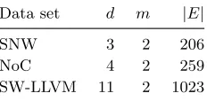
Data set d m |E|
SNW 3 2 206
NoC 4 2 259
SW-LLVM 11 2 1023
Table 1: Data sets used in our experiments.
The main characteristics of the data sets are summarized in Table 1; note that in all casesm= 2. To obtain the ground truth, we completely evaluated all data sets to determine
P in each case. This was very costly, most notably, it took 20 days for NoC alone. The evaluations are plotted in log scale in Fig. 4; the Pareto fronts are emphasized. All the data is normalized such that all objectives are to be maximized.
7.2 Experimental Setup
Our implementation of-PALuses the Gaussian Process Regression and Classification
Tool-box for Matlab (Rasmussen and Nickisch, 2013). In our experiments we used the squared exponential covariance function with automatic relevance determination. The standard deviation of the noiseν is fixed to 0.1. We use
βt1/2 = 1 3
p
2 log(m|E|π2t2/(6δ)),
which is the value suggested in Zuluaga et al. (2013) scaled by 1/3. This factor is empirical and used because the theoretical analysis is too conservative. In Srinivas et al. (2010) 1/5 is used.
All of the experiments were repeated 200 times and the median of the outcomes is shown in the plots. Additionally, several values of= (i)1≤i≤2 were evaluated, wherei is
proportional to the rangeri = maxx∈E{fi(x)}−minx∈E{fi(x)}. We start withi= 0.01×ri
and increase it up toi = 0.3×ri. When we say= 1%, we mean thati is 1% of the range ri.
Prior to running-PAL, a subset of the design space was evaluated in order to initialize
15 points were chosen uniformly at random. For LLVM-SW, as the dimensionality of the design space is much larger, 30 points were taken.
All of the experiments were run on a machine equipped with two 6-Core Intel Xeon X5680 (3.06GHz) and 144GB (1333MHz) of memory.
7.3 Prediction Error
After running -PAL with any of the data sets, a prediction ˆP ⊂E of the true Pareto set
is returned. Some of the points in ˆP are then already evaluated, i.e., f is already known; for the others the exact value of f was not necessary to generate the prediction. For such points, the objective functions are evaluated after running-PALto determine their values
and thus all off( ˆP). We compare the prediction ˆP with the true Pareto setP, wheref(P) is obtained through exhaustive evaluation. The comparison uses a percentage prediction error e(P,Pˆ) based on the concept of -dominance. It is the average maximum distance found between a point in f(P) and the closest point inf( ˆP).
When considering two objective functions, i.e., m = 2, f(x) = (f1(x), f2(x)). In this case, the prediction error is calculated as
e(P,Pˆ) = avgx∈Pminx0∈Pˆmax1≤i≤2
(fi(x)−fi(x0))·100 ri
.
The distance is expressed as a percentage of the range ri, in order to compare the results
between the two dimensions and amongst the different data sets.
7.4 Quality of Pareto Front Prediction
The first row of Fig. 5 shows the -accurate Pareto front Z( ˆP) obtained with -PAL for
three different configurations of , using the first data set. The red shaded line is the true Pareto front found by exhaustive evaluation. The gray points are the ones that have been either sampled during the execution of -PAL or selected to be part of the-Pareto front.
We can see that, as intended, with larger values of, a less accurate Pareto front is obtained, but also fewer points are evaluated. The rest of the points are discarded by-PAL during
its execution.
The second row of Fig. 5 shows equivalent plots obtained with PAL. PAL attempts to classify points as Pareto optimal or not Pareto-optimal until all points have been classified; it uses to ease this classification. Therefore, as increases, more points are selected as Pareto optimal. The gray points in the plots correspond to solutions that are either evaluated during the execution of PAL or classified as Pareto optimal. It is clear that PAL does not generate an -accurate Pareto set, but simply uses a parameter to make the algorithm terminate at different stages. The prediction can be as precise as the models forfi generated with the samples gathered by the termination of the algorithm. For small
0.06 0.08 0.10 0.12 0.14
log(f1) 2 4 6 8 10 12 14 16 log ( f2 )
-PAL with= 1%
0.06 0.08 0.10 0.12 0.14
log(f1) 2 4 6 8 10 12 14 16 log ( f2 )
-PAL with= 12%
0.06 0.07 0.08 0.09 0.10 0.11 0.12 0.13 0.14 0.15
log(f1) 2 4 6 8 10 12 14 16 log ( f2 )
-PAL with= 30%
0.06 0.08 0.10 0.12 0.14
log(f1) 2 4 6 8 10 12 14 16 log ( f2 )
PAL (ICML 2013) with= 1%
0.06 0.08 0.10 0.12 0.14
log(f1) 2 4 6 8 10 12 14 16 log ( f2 )
PAL (ICML 2013) with= 12%
0.06 0.08 0.10 0.12 0.14
log(f1) 2 4 6 8 10 12 14 16 log ( f2 )
PAL (ICML 2013) with= 30%
F( ˆP) F(P)
Figure 5: The first row shows the-accurate Pareto fronts (black line) of the SNW design space obtained with-PALfor∈ {1%,12%,30%}. The second row shows
equiv-alent plots for PAL in which the prediction ˆP is composed of the sampled points and the points classified as Pareto optimal at the termination of the algorithm. The red shaded line in each plots is the true Pareto front of the design space.
Fig. 6 shows a set of experiments in which we do both, exploring the effect of choosing
and comparing against PAL and ParEGO (Knowles, 2006). Every plot in Fig. 6 corresponds to one data set in Table 1. In each case, the x-axis shows the number of evaluations (sampling cost) of f. For -PAL and PAL this is T (the total number of iterations) plus
the evaluations of designs in ˆP that have not been evaluated yet while running the algorithm. On they-axis, we show the average percentage errore(P,Pˆ) as defined above. We measure the error at each iteration, and plot (t, e(P,Pˆ)). As expected, the error in all cases decreases with increasing numbers of evaluations.
-PALprovides a wide range of accuracy-cost trade-offs as an effect of choosing different configurations. When= 30%, only a few iterations are made by the algorithm, returning an error of less than 7% with less than 30 function evaluations in all cases. On the other hand, for = 1%, -PAL yields an error of less than 0.7% with less than 50 function
0 20 40 60 80 100 120 Evaluations 0 1 2 3 4 5 6 7 8 e ( P ,
ˆP)[%]
= 30%
= 1% = 0
SNW (|E|=206)
0 10 20 30 40 50 60 70 80
Evaluations 0 1 2 3 4 5 6 e ( P ,
ˆP)[%]
= 30%
= 1% = 0
NoC (|E|=259)
0 20 40 60 80 100
Evaluations 0 1 2 3 4 5 6 e ( P ,
ˆP)[%]
= 30%
= 1% = 0
SW-LLVM (|E|=1023)
-PAL PAL [ICML 2013] ParEGO
Figure 6: Prediction error e(P,Pˆ) vs. number of evaluations. For -PAL and PAL the
values ∈ {30%,20%,16%,12%,8%,4%,2%,1%} are used. The corresponding points are consecutive in the lines for-PALand PAL.
The measured error e(P,Pˆ) is comparable with as they both measure how far the predicted Pareto front is from the true Pareto front. measures the desired accuracy, and
e(P,Pˆ) measures what is obtained. We can then say that -PAL meets the expectations
on the prediction for allconfigurations and in all cases.
The plots in Fig. 6 also show a point in which -PAL achieves an error of 0. This is
obtained with= 0,δ= 0.05 andβthaving the exact value suggested by Theorem 1. Under
these configurations,-PAL yields a perfect prediction with less than 115 evaluations in all
cases.
PAL (purple line) generates a more constrained set of trade-offs using the same con-figurations that were used for -PAL. The actual ˆP reported in (Zuluaga et al., 2013)
corresponds to the Pareto-optimal points amongst all pairs (µ1(x), µ2(x)) for x ∈E. On the other hand, ParEGO (gray line) does not provide a methodology to stop the algorithm in different stages of accuracy and cost. We then plot a continuous line that shows the error obtained by the set St of sampled points on every iteration of the algorithm t, i.e.,
we plot points (|St|, e(P, St)). ParEGO uses a heuristic to find the number of samples of
the starting population depending on the characteristics of the design space. Hence the line always starts with a certain minimum number of evaluations.
We observe that -PAL and PAL in all cases significantly improve over ParEGO. In
particular, the gains on SW-LLVM were considerable. Overall, the number of evaluations was reduced by 1/3 to 2/3 in all cases when comparing against ParEGO. -PAL overall
As explained above, -PAL returns an -accurate Pareto set and PAL returns a more
dense Pareto set, therefore, the prediction error in PAL is always fairly small and in most of the cases it requires more function evaluations. In the case of SW-LLVM, there are some trade-offs obtained with-PAL that yield slightly higher errors than those obtained
with PAL. This is because-PALeliminates solutions along its execution and as the
corre-sponding design space has only one Pareto point, when this is removed, the error obtained increases considerably. However the error is within the expected range, i.e., below that indicated by . Additionally, if the design space is not too large, after the termination of the algorithm, all points that were discarded can be again predicted by the model to find a more accurate Pareto set similar to what PAL returns.
In conclusion, -PAL in most cases produces better trade-offs than PAL and ParEGO.
In comparison to PAL, it uses more effectively the fact that the users, by setting , are expressing their desire to generate only-accurate Pareto fronts in exchange for a smaller number of function evaluations. This means that it can offer a wider range of trade-offs between accuracy and number of evaluations. Moreover, the resulting Pareto fronts contain a variety of trade-offs between the underlying multi-objective design space, that are spread evenly along the range of possibilities.
7.5 Execution Time
A drawback of PAL is the high number of computations required per iteration, which constrains it to small design spaces. As explained in Section 6, -PAL reduces the number
of computations per iteration by a factor of nwhile achieving better results than PAL. In this section, we compare the runtime of executing PAL and-PALwith our three data sets.
Another advantage of -PAL that helps improving its computational efficiency is that it
uses to discard more points from the design space as its value increases. In PAL on the other hand, asincreases, the number of points classified as Pareto optimal increases, and thus those points require computations on every iteration until the algorithm terminates.
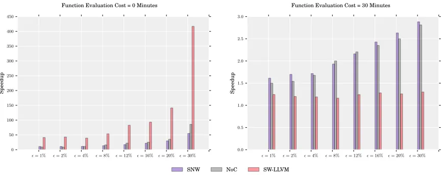
The first plot in Fig. 7 shows runtime speedups, obtained with the three data sets and all the values of considered before. We measured for each value of the runtime for
-PAL and PAL and divide them to obtain the speedups. Here we assume that the cost of
evaluating f is 0. The plot shows that, as expected, the speedups improve as n increases. Therefore, LLVM-SW, which has the largest design space of all data sets, obtains the largest speedups, from 45×with = 1% up to 420×with= 30%. Better speedups are obtained with larger values ofsince more points can be discarded during the first iterations.
The second plot in Fig. 7 shows equivalent results but this time assuming that evaluating
f takes 30 minutes. In this case, the speedups are smaller, going up to almost 3× for
= 30%. This is because the data sets are relatively small and thus the gains in runtime are offset by the high cost of evaluating f. In other words, the speedups that we observed here are speedups on function evaluations and are related to the improvements that can be visualized in Fig. 6. These improvements come from the fact that -PAL requires less
function evaluations than PAL to achieve an error equivalent to the requested. As a result, the denser the true Pareto front of the design space, the better the speedups obtained by using-PAL. For this reason, LLVM-SW does not generate important speedups on function
= 1% = 2% = 4% = 8% = 12% = 16% = 20% = 30% 0
50 100 150 200 250 300 350 400 450
Speedup
Function Evaluation Cost = 0 Minutes
= 1% = 2% = 4% = 8% = 12% = 16% = 20% = 30% 0.0
0.5 1.0 1.5 2.0 2.5 3.0
Speedup
Function Evaluation Cost = 30 Minutes
SNW NoC SW-LLVM
Figure 7: Speedups obtained by using-PALagainst using PAL. The plot of the left shows
the speedups on the runtime of -PAL, assuming that function evaluations are
free. The plot on the right shows speedups assuming that one function evaluation takes 30 minutes.
are obtained with SNW, followed by NoC, tha same order as the densities of their true Pareto curves.
8. Conclusions
In this paper, we proposed a novel algorithm for efficiently localizing an-accurate Pareto-frontier in multi-objective optimization. In the spirit of Bayesian optimization, it uses Gaussian processes to exploit prior information about the objective functions’ regularity to predict the objective functions, to guide the sampling process, and to make inferences about the optimality of designs without directly evaluating them. We presented an extensive theoretical analysis including bounds for the number of samples required to achieve the desired target accuracy.
The algorithm described in this paper presents major improvements from its predecessor PAL. First, it returns an -accurate Pareto front instead of a dense approximation of the true Pareto front. It is often the case that a small difference in the objective function, conveyed to the algorithm with the parameter , does not affect the quality of a design significantly. Thus, it is preferable to reduce the number of evaluations made and to obtain a set of close-to-optimal solutions well distributed in the objective space.
A second improvement over PAL is that-PALreduces the asymptotic runtime, which
facilitates the exploration of larger design spaces, in which perhaps the function evaluation is less expensive.
evaluations. Moreover, we showed that our parameterization strategy provides a wide range of cost-performance trade-offs. In comparison to PAL, our experiments show that -PAL
reduces the amount of computations by up to 420×, and the number of samples from the design space required to meet the user’s desired level of accuracy by up to 2.9×.
Acknowledgments. We would like to thank the authors of (Almer et al., 2011) and (Siegmund et al.,
Appendix A. Theoretical Analysis and Asymptotic Bounds
This section provides the proofs of Theorem 1, which follows from Lemmas 1 to 8.
Lemma 1 Assume that the target functions fi, 0 ≤ i ≤ m, are bounded on their RKHS
norm ||fi||k. Given δ ∈ (0,1) and βt = 2||fi||2k+ 300γtlog3(m|E|t/δ), the following holds
with probability≥1−δ:
|fi(x)−µt−1,i(x)| ≤βt1/2σt−1,i(x)
for all 1≤i≤m, x∈E, for allt≥1. (10)
In other words, with probability≥1−δ:
f(x)∈Rt(x) for allx∈E, for all t≥1
Proof According to Theorem 6 in (Srinivas et al., 2012), the following inequality holds:
P rn|fi(x)−µt−1,i(x)|> βt1/2σt−1,i(x)
o ≤δ0,
withβt= 2||fi||2k+ 300γtlog3(t/δ0). Applying the union bound for i, t∈N, we obtain that
the following holds with probability≥1−m|E|δ0:
|fi(x)−µt−1,i(x)| ≤βt1/2σt−1,i(x)
for all 1≤i≤m, for all x∈E, (11)
withβt= 2||fi||2k+ 300γtlog3(t/δ0). The lemma holds by choosingδ =m|E|δ0.
Lemma 2 If m= 1 and fT = (f(xt))1≤t≤T, then
I(yT;fT) = 1 2
T
X
t=1
log(1 +σ−2σt2−1(xt)).
This is directly taken from Lemma 5.3 in (Srinivas et al., 2010). Hereby I(yT;fT) =
H(fT)−H(fT | (x1,y1), . . . ,(xT,yT)) is the mutual information between the function
values fT and the noisy observations yT = fT +νT where where νT ∼ N(0, σ2I). This
relation holds no matter in what sequence the samples xt are picked by -PAL, and no
matter what values yt are being observed. Latter statement is true since for Gaussian processes the posterior variance over f only depends on where it is evaluated, i.e., xT, not on the actual values yT observed (Srinivas et al., 2010).
Lemma 3 Given δ ∈(0,1)and βt= 2 log(m|E|πt/δ), the following holds: T
X
t=1
w2t ≤βTC1I(yT;fT)≤C1βTγT for allT ≥1,
Proof One of the rectangles of which Rt(xt) is the intersection has a diagonal length of
2βt1/2kσt−1(xt)k2: as a consequence,
w2t ≤4βtkσt−1(xt)k22. Asβt is increasing, we have that
w2t ≤ 4βTσ2 m
X
i=1
σ−2σt2−1,i(xt)
≤ 4βTσ2C2
m
X
i=1
log(1 +σ−2σ2
t−1,i(xt))
with C2 = σ−2/log(1 + σ−2) ≥ 1, since s2 ≤ C2log(1 + s2) for 0 ≤ s ≤ σ−2, and
σ−2σ2
t−1,i(xt)≤σ−2ki(xt,xt)≤σ−2.
UsingC1 = 8σ2C2 and Lemma 2 we have that
T
X
t=1
w2t ≤ βTC1
m
X
i=1
I(yT;fT,i)
≤ βTC1I(yT;fT)
Lemma 4 Given δ ∈(0,1) and βt= 2 log(m|E|πt/δ), the following holds with probability
≥1−δ:
T
X
t=1
wt≤
p
C1T βTγT for all T ≥1
Proof This follows from Lemma 3, since (PT
t wt)2 ≤TPTt=1w2t by the Cauchy-Schwarz
inequality.
Lemma 5 Running -PAL with a monotonic classification, it holds thatwtdecreases with t.
Proof As a direct consequence of the sample selection rule,wt−1(xt)≤wt−1. On the other hand,wt(x)≤wt−1(x) and thus,wt≤wt−1(xt). The lemma follows.
Lemma 6 Running -PAL with δ∈(0,1)and βt= 2 log(m|E|πt/δ), the following holds:
P r
(
wT ≤
r
C1βTγT
T for all T ≥1
)
≥1−δ, (12)
Proof This is derived from Lemmas 4 and 5, since PT
t=1wt/T ≥wT.
Lemma 7 If when running -PAL, wt ≤ ||||∞ holds at iteration t, then the algorithm
terminates without further sampling.
Proof Sincewt is un upper bound of ||max(Rt(x))−min(Rt(x))||2, it is enough to show that the statement is true if w = max(Rt(xi))−min(Rt(xi)) = (w(1)t , . . . , w
(m)
t ) for all xi∈Ut∪Pt. Therefore, wt≤ ||||∞ implies w.
We show that if w , in the same iteration of -PAL all points in Ut will be either
moved toPt or discarded.
If a point xdoes not belong to Z(E), then there is a pointx0 such that
max(Rt(x0))min(Rt(x)) +.
Using max(Rt(x0)) = min(Rt(x0)) +w, we can rewrite
min(Rt(x)) +min(Rt(x0)) +w.
Since w, this is equivalent to
min(Rt(x)) +wmin(Rt(x0)) +.
It follows that
max(Rt(x))min(Rt(x0)) +,
which is the condition that ensures thatx x0. This means that there is a pointx0 ∈Ut∪Pt
that dominates x, and thereforexwill be discarded.
Lemma 8 If -PAL is run until its termination with some and confidence parameterδ,
then with probability at least 1−δ it holds thatΠ( ˆP) is an -accurate Pareto set of E.
Proof According to Definition 5, an-accurate Pareto set of E requires every point of E
to have an -dominator in ˆP. In the discarding stage of-PAL, points inUt are discarded
if they are -dominated by a pessimistic Pareto point. If a point is -dominated in E, it is -dominated by a point in the pessimistic Pareto set of E. Therefore, the discarding stage of -PAL ensures that there will be always be a point in the remaining sets that -dominates the points that are discarded. Pessimistic Pareto points are only discarded if they are -dominated by any point in Pt. Hence, all discarding decisions are “safe”, in
the sense that for every discarded point, there is always at least one -dominating point remaining. They are also “complete”, i.e., only points that belong to Z(E) are moved to Pt. Hence, at termination, since Ut is empty, all remaining points Pt form an -accurate
References
O. Almer, N. Topham, and B. Franke. A learning-based approach to the automated design of MPSoC networks. Architecture of Computing Systems (ARCS), pages 243–258, 2011.
R. Bardenet, M. Brendel, B. K´egl, and M. Sebag. Collaborative hyperparameter tuning. In
Intl. Conference on Machine Learning (ICML), pages 199–207, 2013.
E. Bonilla, K. M. A. Chai, and C. K. I. Williams. Multi-task Gaussian process prediction. In
Advances in Neural Information Processing Systems (NIPS), volume 20, pages 153–160, 2008.
S. Boyd and L. Vandenberghe. Convex Optimization. Cambridge University Press, 2004.
E. Brochu, V. M. Cora, and N. de Freitas. A tutorial on Bayesian optimization of expensive cost functions, with application to active user modeling and hierarchical reinforcement learning. Arxiv preprint arXiv:1012.2599, 2010.
D. Buche, N. N. Schraudolph, and P. Koumoutsakos. Accelerating evolutionary algorithms with Gaussian process fitness function models. IEEE Trans. on Systems, Man, and Cybernetics, 35:183–194, 2005.
A. Bull. Convergence rates of efficient global optimization algorithms. Journal of Machine Learning Research, 12:2879–2904, 2011.
P. Campigotto, A. Passerini, and R Battiti. Active learning of Pareto fronts. IEEE Trans. on Neural Networks and Learning Systems, 25:506–519, 2014.
C. Coello, G. B. Lamont, and D. Veldhuizen. Evolutionary algorithms for solving multi-objective problems. Springer, 2006.
D. D. Cox and S. John. SDO: A statistical method for global optimization.Multidisciplinary Design Optimization: State of the Art, pages 315–329, 1997.
N. de Freitas, A. Smola, and M. Zoghi. Exponential regret bounds for Gaussian process ban-dits with deterministic observations. In Intl. Conference on Machine Learning (ICML), pages 1743–1750, 2012.
L. Deng, K. Sobti, and C. Chakrabarti. Accurate models for estimating area and power of FPGA implementations. In Intl. Conference on Acoustics, Speech and Signal Processing (ICASSP), pages 1417–1420, 2008.
M. T. M. Emmerich, K. C. Giannakoglou, and B. Naujoks. Single- and multiobjective evolutionary optimization assisted by Gaussian random field metamodels. IEEE Trans. on Evolutionary Computation, 10(4):421–439, 2006.
M. A. Gelbart, J. Snoek, and R. P. Adams. Bayesian optimization with unknown constraints. In Uncertainty In Artificial Intelligence (UAI), 2014.