Characteristic and Universal Tensor Product Kernels

Characteristic and Universal Tensor Product Kernels

Zolt´an Szab´o [email protected]

CMAP, ´Ecole Polytechnique

Route de Saclay, 91128 Palaiseau, France

Bharath K. Sriperumbudur [email protected]

Department of Statistics Pennsylvania State University 314 Thomas Building

University Park, PA 16802

Editor:Francis Bach

Abstract

Maximum mean discrepancy (MMD), also called energy distance or N-distance in statis-tics and Hilbert-Schmidt independence criterion (HSIC), specifically distance covariance in statistics, are among the most popular and successful approaches to quantify the dif-ference and independence of random variables, respectively. Thanks to their kernel-based foundations, MMD and HSIC are applicable on a wide variety of domains. Despite their tremendous success, quite little is known about when HSIC characterizes independence and when MMD with tensor product kernel can discriminate probability distributions. In this paper, we answer these questions by studying various notions of characteristic property of the tensor product kernel.

Keywords: tensor product kernel, kernel mean embedding, characteristic kernel, I-characteristic kernel, universality, maximum mean discrepancy, Hilbert-Schmidt indepen-dence criterion

1. Introduction

Kernel methods (Sch¨olkopf and Smola, 2002) are among the most flexible and influential tools in machine learning and statistics, with superior performance demonstrated in a large number of areas and applications. The key idea in these methods is to map the data samples into a possibly infinite-dimensional feature space—precisely, a reproducing kernel Hilbert space (RKHS; Aronszajn, 1950)—and apply linear methods in the feature space, without the explicit need to compute the map. A generalization of this idea to probability measures, i.e., mapping probability measures into an RKHS (Berlinet and Thomas-Agnan, 2004, Chapter 4; Smola et al., 2007) has found novel applications in nonparametric statistics and machine learning. Formally, given a probability measure P defined on a measurable spaceXand an RKHSHkwithk:X×X→Ras the reproducing kernel (which is symmetric and positive definite),P is embedded into Hk as

P7→

Z

Xk(

·, x) dP(x) =:µk(P), (1)

c

where µk(P) is called the mean element or kernel mean embedding of P. The mean

em-bedding of P has lead to a new generation of solutions in two-sample testing (Baringhaus and Franz, 2004; Sz´ekely and Rizzo, 2004, 2005; Borgwardt et al., 2006; Harchaoui et al., 2007; Gretton et al., 2012), goodness-of-fit testing (Chwialkowski et al., 2016; Liu et al., 2016; Jitkrittum et al., 2017b; Balasubramanian et al., 2017), domain adaptation (Zhang et al., 2013) and generalization (Blanchard et al., 2017), kernel belief propagation (Song et al., 2011), kernel Bayes’ rule (Fukumizu et al., 2013), model criticism (Lloyd et al., 2014; Kim et al., 2016), approximate Bayesian computation (Park et al., 2016), probabilistic pro-gramming (Sch¨olkopf et al., 2015), distribution classification (Muandet et al., 2011; Zaheer et al., 2017), distribution regression (Szab´o et al., 2016; Law et al., 2018) and topological data analysis (Kusano et al., 2016). A recent survey on the topic is provided by Muandet et al. (2017).

Crucial to the success of the mean embedding based representation is whether it en-codes all the information about the distribution, in other words whether the map in (1) is injective in which case the kernel is referred to as characteristic (Fukumizu et al., 2008; Sriperumbudur et al., 2010). Various characterizations for the characteristic property of k is known in the literature (Fukumizu et al., 2008, 2009; Sriperumbudur et al., 2010; Gretton et al., 2012) using which the popular kernels on Rd such as Gaussian, Laplacian, B-spline, inverse multiquadrics, and the Mat´ern class are shown to be characteristic. The charac-teristic property is closely related to the notion of universality (Steinwart, 2001; Micchelli et al., 2006; Carmeli et al., 2010; Sriperumbudur et al., 2011)—k is said to be universal if the corresponding RKHS Hk is dense in a certain target function class, for example, the

class of continuous functions on compact domains—and the relation between these notions has recently been explored by Sriperumbudur et al. (2011); Simon-Gabriel and Sch¨olkopf (2016).

Based on the mean embedding in (1), Smola et al. (2007) and Gretton et al. (2012) defined a semi-metric, called the maximum mean discrepancy (MMD) on the space of probability measures:

MMDk(P,Q) :=kµk(P)−µk(Q)kHk,

which is a metric iff k is characteristic. A fundamental application of MMD is in non-parametric hypothesis testing that includes two-sample (Gretton et al., 2012) and inde-pendence tests (Gretton et al., 2008). Particularly in indeinde-pendence testing, as a measure of independence, MMD measures the distance between the joint distributionPXY and the

product of marginals PX ⊗PY of two random variables X and Y which are respectively

defined on measurable spacesXandY, with the kernelkbeing defined onX×Y. As afore-mentioned, if kis characteristic, then MMDk(PXY,PX⊗PY) = 0 impliesPXY =PX ⊗PY,

i.e., X and Y are independent. A simple way to define a kernel on X×Y is through the tensor product of kernels kX and kY defined on X and Y respectively: k =kX ⊗kY, i.e.,

k((x, y),(x0, y0)) = kX(x, x0)kY(y, y0), x, x0 ∈ X, y, y0 ∈ Y, with the corresponding RKHS

Hk =HkX⊗HkY being the tensor product space generated by HkX andHkY. This means,

when k=kX ⊗kY,

MMDk(PXY,PX ⊗PY) =kµkX⊗kY(PXY)−µkX⊗kY(PX ⊗PY)kH_kX⊗H_kY . (2)

In addition to the simplicity of defining a joint kernelkonX×Y, the tensor product kernel

correspond to different modalities (say images, texts, audio). By exploiting the isomorphism between tensor product Hilbert spaces and the space of Hilbert-Schmidt operators1, it follows from (2) that

MMDk(PXY,PX ⊗PY) =kCXYkHS=: HSICk(PXY), (3)

which is the Hilbert-Schmidt norm of the cross-covariance operatorCXY :=µkX⊗kY(PXY)−

µkX(PX)⊗µkY(PY) and is known as the Hilbert-Schmidt independence criterion (HSIC)

(Gretton et al., 2005a). HSIC has enjoyed tremendous success in a variety of applications such as independent component analysis (Gretton et al., 2005a), feature selection (Song et al., 2012), independence testing (Gretton et al., 2008; Jitkrittum et al., 2017a), post selection inference (Yamada et al., 2018) and causal detection (Mooij et al., 2016; Pfister et al., 2017; Strobl et al., 2017). Recently, MMD and HSIC (as defined in (3) for two components) have been shown by Sejdinovic et al. (2013b) to be equivalent to other popular statistical measures such as the energy distance (Baringhaus and Franz, 2004; Sz´ekely and Rizzo, 2004, 2005)—also known as N-distance (Zinger et al., 1992; Klebanov, 2005)—and distance covariance (Sz´ekely et al., 2007; Sz´ekely and Rizzo, 2009; Lyons, 2013) respectively. HSIC has been generalized toM ≥2 components (Quadrianto et al., 2009; Sejdinovic et al., 2013a) to measure the joint independence of M random variables

HSICk(P) =

µ⊗M_m=1km(P)− ⊗

M

m=1µkm(Pm)

_⊗M

m=1Hkm

, (4)

where P is a joint measure on the product space X := ×Mm=1Xm and (Pm)Mm=1 are the marginal measures of P defined on (Xm)Mm=1 respectively. The extended HSIC measure has recently been analyzed in the context of independence testing (Pfister et al., 2017). In addition to testing, the extended HSIC measure is also useful in the problem of inde-pendent subspace analysis (ISA; Cardoso, 1998), wherein the latent sources are separated by maximizing the degree of independence among them. In all the applications of HSIC, the key requirement is that k = ⊗M

m=1km captures the joint independence of M random

variables (with joint distribution P)—we call this property as I-characteristic—, which is guaranteed ifkis characteristic. Sincekis defined in terms of (km)Mm=1, it is of fundamental importance to understand the characteristic and I-characteristic properties of k in terms of the characteristic property of (km)Mm=1, which is one of the main goals of this work.

For M = 2, the characterization of independence, i.e., the I-characteristic property of k, is studied by Blanchard et al. (2011) and Gretton (2015) where it has been shown that if k1 and k2 are universal, thenk is universal2 and therefore HSIC captures independence. A stronger version of this result can be obtained by combining (Lyons, 2013, Theorem 3.11) and (Sejdinovic et al., 2013b, Proposition 29): if k1 and k2 are characteristic, then the HSIC associated with k = k1⊗k2 characterizes independence. Apart from these results, not much is known about the characteristic/I-characteristic/universality properties ofkin

1. In the equivalence one assumes thatHk_X,Hk_Y are separable; this holds under mild conditions, for exam-ple ifXandYare separable topological domains andkX,kY are continuous (Steinwart and Christmann, 2008, Lemma 4.33).

terms of the individual kernels. Our goal is to resolve this question and understand the characteristic, I-characteristic and universal property of the product kernel (⊗M

m=1km) in

terms of the kernel components ((km)Mm=1) for M ≥2. Because of the relatedness of MMD and HSIC to energy distance and distance covariance, our results also contribute to the better understanding of these other measures that are popular in the statistical literature. Specifically, our results shed light on the following surprising phenomena of the I -characteristic property of⊗M

m=1km forM ≥3:

1. characteristic property of (km)Mm=1 is not sufficient but necessary for ⊗Mm=1km to be

I-characteristic;

2. universality of (km)Mm=1 is sufficient for⊗Mm=1km to beI-characteristic, and

3. if at least one of (km)Mm=1 is only characteristic and not universal, then⊗Mm=1km need

not beI-characteristic.

The paper is organized as follows. In Section 3, we conduct a comprehensive analysis about the above mentioned properties ofkand (km)Mm=1 for any positive integerM. To this end, we define various notions of characteristic property on the product spaceX(see Defini-tion 1 and Figure 2(a) in SecDefini-tion 3) and explore the relaDefini-tion between them. In order to keep our presentation in this section to be non-technical, we relegate the problem formulation to Section 3, with the main results of the paper being presented in Section 4. A summary of the results is captured in Figure 1 while the proofs are provided in Section 5. Various definitions and notation that are used throughout the paper are collected in Section 2.

2. Definitions and Notation

N:={1,2, . . .}andRdenotes the set of natural numbers and real numbers respectively. For M ∈N, [M] :={1, . . . , M}. 1d:= (1,1, . . . ,1)∈Rdand 0 denotes the matrix of zeros. For a:= (a1, . . . , ad)∈Rd and b := (b1, . . . , bd) ∈Rd,ha, bi=Pdi=1aibi is the Euclidean inner product. For setsAandB,A\B={a∈A:a /∈B}is their difference,|A|is the cardinality of A and ×M

m=1Am = {(a1, . . . , aM) : am ∈ Amm ∈[M]} is the Descartes product of sets

(Am)Mm=1. P(X) denotes the power set of a setX, i.e., all subsets ofX(including the empty set and X). The Kronecker delta is defined as δa,b = 1 if a=b, and zero otherwise. χA is

the indicator function of setA: χA(x) = 1 if x∈A andχA(x) = 0 otherwise. Rd1×...×dM _is

the set ofd1×. . .×dM-sized tensors.

For a topological space (X, τ_X),B(X) :=B(τ_X) is the Borel sigma-algebra onXinduced by the topologyτ_X. Probability and finite signed measures in the paper are meant w.r.t. the measurable space (X,B(X)). Given {(Xi, τi)}i∈I topological spaces, their product ×i∈IXi

is enriched with the product topology; it is the coarsest topology for which the canonical projectionsπi :×i∈IXi →(Xi, τi) are continuous for alli∈I. A topological space (X, τX) is

called second-countable ifτ_X has a countable basis.3 C(X) denotes the space of continuous functions on X. C0(X) denotes the class of real-valued functions vanishing at infinity on a locally compact Hausdorff (LCH) space4 X, i.e., for any >0, the set{x ∈X:|f(x)| ≥} 3. Second-countability implies separability; in metric spaces the two notions coincide (Dudley, 2004, Propo-sition 2.1.4). By the Urysohn’s theorem, a topological space is separable and metrizable if and only if it is regular, Hausdorff and second-countable. Any uncountable discrete space isnot second-countable. 4. LCH spaces includeRd, discrete spaces, and topological manifolds. Open or closed subsets, finite

⊗0-char ⊗-char char c0-universal

I-char

(km)Mm=1 char (km)Mm=1 c0-universal

(8)

Remark

2(

iii

)

(8)

Remark 7

(8)

(8)

/

Example 1

Theorem

5

/

Example 1

/

Example 1

Theorem

3 (M=2) /

Example 2 (M

≥3)

/ Sriperumbudur et al. (2011)

Theorem 3

Sriperumbudur et al. (2011)

Figure 1: Summary of results: “char” denotes characteristic. In addition to the usual characteristic property, three new notions⊗0-characteristic,⊗-characteristic and

I-characteristic are introduced in Definition 1 which along with c0-universal (in the top right corner) correspond to the property of the tensor product kernel

⊗M

m=1km, while the bottom part of the picture corresponds to the individual

kernels (km)Mm=1being characteristic orc0-universal. If (km)Mm=1-s are continuous, bounded and translation invariant kernels onRdm, m ∈[M], all the notions are equivalent (see Theorem 4).

is compact. C0(X) is endowed with the uniform norm kfk∞ = supx∈X|f(x)|. Mb(X) and

M+

1(X) are the space of finite signed measures and probability measures onX, respectively. ForPm ∈M+₁(Xm),⊗Mm=1Pm denotes the product probability measure on the product space

×M

m=1Xm, i.e., ⊗Mm=1Pm ∈ M+1(×Mm=1Xm). δx is the Dirac measure supported on x ∈ X.

For F ∈ Mb ×Mm=1Xm

, the finite signed measure Fm denotes its marginal on Xm. Hkm

is the reproducing kernel Hilbert space (RKHS) associated with the reproducing kernel km :Xm×Xm →R, which in this paper is assumed to be measurable and bounded. The tensor product of (km)Mm=1 is a kernel, defined as

⊗M_m=1km (x1, . . . , xM), x01, . . . , x 0

M

=

M Y

m=1

km xm, x0m

, xm, x0m∈Xm,

whose associated RKHS is denoted asH_⊗M

m=1km=⊗

M

m=1Hkm(Berlinet and Thomas-Agnan,

2004, Theorem 13), where the r.h.s. is the tensor product of RKHSs (Hkm)

M

m=1. For hm ∈

Hm,m∈[M], the multi-linear operator⊗mM=1hm∈ ⊗Mm=1Hm is defined as

⊗M_m=1hm

(v1, . . . , vM) = M Y

m=1

A kernel k :X×X→ _R defined on a LCH space X is called a c0-kernel if k(·, x)∈ C0(X) for all x ∈ X. k : Rd ×Rd → R is said to be a translation invariant kernel on Rd if k(x, y) =ψ(x−y), x, y∈_Rd _{for a positive definite functionψ:}

Rd→R. µk(F) denotes the kernel mean embedding of F ∈Mb(X) to Hk which is defined as µk(F) = R_Xk(·, x) dF(x), where the integral is meant in the Bochner sense.

3. Problem Formulation

In this section, we formally introduce the goal of the paper. To this end, we start with a definition. For simplicity, throughout the paper, we assume that all kernels are bounded. The definition is based on the observation (Sriperumbudur et al., 2010, Lemma 8) that a bounded kernelk on a topological space (X, τ_X) is characteristic if and only if

Z

X

Z

Xk(x, x 0_{) d}

F(x) dF(x0)>0, ∀F∈Mb(X)\{0} such thatF(X) = 0.

In other words, characteristic kernels are integrally strictly positive definite (ispd; see Sripe-rumbudur et al., 2010, p. 1523) w.r.t. the class of finite signed measures that assign zero measure to X. The following definition extends this observation to tensor product kernels on product spaces.

Definition 1 (F-ispd tensor product kernel)Suppose km:Xm×Xm→Ris a bounded

kernel on a topological space(Xm, τ_Xm), m∈[M]. LetF⊆Mb(X)be such that0∈Fwhere

X:=×M

m=1Xm. k:=⊗Mm=1km is said to be F-ispd if

µk(F) = 0⇒F= 0 (F∈F), or equivalently

kµk(F)k2_Hk =

Z

×M m=1Xm

Z

×M m=1Xm

⊗M_m=1km

x, x0 dF(x) dF(x0)>0, ∀F∈F\{0}. (5)

Specifically,

• ifkm-s arec0-kernels on locally compact Polish (LCP)5 spaces Xm-s andF=Mb(X),

thenk is called c0-universal.

• if

F= [Mb(X)]0 :={F∈Mb(X) :F(X) = 0},

F=⊗M_m=1Mb(Xm) 0

:=F∈ ⊗Mm=1Mb(Xm),F(X) = 0 ,

F=I :=P− ⊗Mm=1Pm :P∈M+1 ×Mm=1Xm , (M ≥2)

F=⊗M_m=1M0_b(Xm) :=

F=⊗Mm=1Fm : Fm ∈Mb(Xm),Fm(Xm) = 0, ∀m∈[M] ,

thenkis called characteristic,⊗-characteristic,I-characteristicand ⊗₀-characteristic, respectively.

5. A topological space is called Polish if it is complete, separable and metrizable. For example, Rd and

In Definition 1, k being characteristic matches the usual notion of characteristic kernels on a product space, i.e., there are no two distinct probability measures on X =×M

m=1Xm

such that the MMD between them is zero. The other notions such as ⊗-characteristic,

I-characteristic and ⊗₀-characteristic are typically weaker than the usual characteristic property since

⊗M

m=1M0b(Xm) ⊆

⊗M

m=1Mb(Xm) 0

⊆ M_b ×M_m=1X_m0 ⊆ M_b ×M_m=1X_m

I

⊆

. (6)

Below we provide further intuition on the Fmeasure classes enlisted in Definition 1.

Remark 2 (i) F=Mb(X) : If km-s are c0-kernels on LCH spaces Xm for all m ∈[M],

then k is also a c0-kernel on LCH spaceX implying that ifk satisfies (5), then kis c0 -universal (Sriperumbudur et al., 2010, Proposition 2). It is well known (Sriperumbudur et al., 2010) thatc0-universality reduces toc-universality (i.e., the notion of universality

proposed by Steinwart, 2001) if X is compact which is guaranteed if and only if each

Xm, m∈[M]is compact.

(ii) F=I :This family is useful to describe the joint independenceofM random variables— hence the name I-characteristic—defined on kernel-endowed domains (Xm)Mm=1: If P

denotes the joint distribution of random variables (Xm)Mm=1 and (Pm)Mm=1 are the

asso-ciated marginals on (Xm)Mm=1, then by definition k=⊗Mm=1km is I-characteristic iff

HSICk(P) = 0⇐⇒P=⊗Mm=1Pm.

In other words, HSIC captures joint independence exactly with I-characteristic kernels. Similarly, the I-characteristic property ensures that COCO (constrained covariance; Gretton et al., 2005b) is a joint independence measure as COCO is defined by replacing the Hilbert-Schmidt norm of the cross-covariance operator (see (3) and (4)) with its spectral norm.

(iii) F = ⊗M

m=1M0b(Xm) : In this case F is chosen to be the product of finite signed measures on X such that each marginal measure Fm assigns zero to the

correspond-ing space Xm. This choice is relevant as the characteristic property of individual

ker-nels (km)Mm=1 need not imply the characteristic property of ⊗Mm=1km, but is

equiva-lent to the ⊗0-characteristic property of ⊗Mm=1km. The equivalence holds for bounded

kernels km : Xm × Xm → R on topological spaces Xm (m ∈ [M]) since for any

F=⊗Mm=1Fm ∈ ⊗Mm=1Mb(Xm),Fm(Xm) = 0 (∀m∈[M])

kµk(F)k2_H

⊗M m=1km

=

M Y

m=1

kµkm(Fm)k

2

Hkm, (7)

and the l.h.s. is positive iff each term on the r.h.s. is positive.

(iv) F =

⊗M

m=1Mb(Xm)

0

: This class is similar to the one discussed in (iii) above— i.e., class of product measures—with the slight difference that the joint measure F is

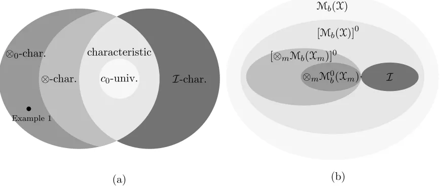
c0-univ. characteristic

I-char.

⊗-char.

⊗₀-char.

(a) Example 1

Mb(X)

[Mb(X)]0

I ⊗mM0_b(Xm)

[⊗mMb(Xm)]0

(b)

Figure 2: (a) F-ispd ⊗M

m=1km kernels (see (8)); (b) F ⊆ Mb(X), X = ×Mm=1Xm.

Exam-ple 1: ⊗M

m=1km is ⊗0-characteristic but not ⊗-characteristic and therefore not characteristic.

to assign zero measure to the corresponding space Xm. While the need for considering

such a measure class may not be clear at this juncture, however, based on (7), it turns out that this choice of F has quite surprising connections to the characteristic property and c0-universality of the product kernel; for details see Remark 7.

(v) F-ispd relations: Given the relations in (6), it immediately follows that k=⊗M m=1km

satisfies

⊗₀-characteristic ⇐= ⊗-characteristic ⇐= _{characteristic}

⇐

c0-universal ⇐=

I-characteristic

(8)

when Xm for all m ∈[M] are LCP. A visual illustration of (6) and (8) is provided in

Figure 2.

(vi)

⊗M

m=1Mb(Xm)

0

∩I={0}:While it is clear that

⊗M

m=1Mb(Xm) 0

andIare subsets

of Mb(×Mm=1Xm) 0

, it is interesting to note that ⊗M

m=1Mb(Xm) 0

and I have a trivial intersection with 0 being the measure common to each of them, assuming thatXm-s are

second-countable for all m∈[M]; see Section 5.1.

Having defined theF-ispd property, our goalis to investigate whether the characteristic or c0-universal property of km-s (m∈[M]) imply differentF-ispd properties of⊗Mm=1km, and

vice versa.

4. Main Results

(LCH) and locally compact Polish (LCP), so that they are presented in more generality. However, for simplicity, all these assumptions can be unified by simply assuming a stronger condition thatXm’s are LCP.

Our first example illustrates that the characteristic property of km-s does not imply the

characteristic property of the tensor product kernel. In light of Remark 2(iv) of Section 3, it follows that the class of ⊗₀-characteristic tensor product kernels form a strictly larger class than characteristic tensor product kernels; see also Figure 2.

Example 1 Let X1=X2 ={1,2}, τ_X1 =τ_X2 =P({1,2}), k1(x, x0) =k2(x, x0) = 2δx,x0−1. It is easy to verify that k1 andk2 are characteristic. However, it can be proved that k1⊗k2

is not ⊗-characteristic and therefore not characteristic. On the hand, interestingly, k1⊗k2

is I-characteristic. We refer the reader to Section 5.2 for details.

In the above example, we showed that the tensor product of k1 and k2 (which are characteristic kernels) is I-characteristic. The following result generalizes this behavior for any bounded characteristic kernels. In addition, under a mild assumption, it shows the converse to be true for anyM.

Theorem 3 Let km : Xm×Xm → R be bounded kernels on topological spaces Xm for all

m∈[M], M ≥2. Then the following holds.

(i) Suppose Xm is second-countable for all m ∈ [M] with M = 2. If k1 and k2 are

characteristic, then k1⊗k2 is I-characteristic.

(ii) SupposeXmis Hausdorff and|Xm| ≥2for allm∈[M]. If⊗Mm=1kmisI-characteristic,

thenk1, . . . , kM are characteristic.

Lyons (2013) has showed an analogous result to Theorem 3(i) for distance covariances (M = 2) on metric spaces of negative type (Lyons, 2013, Theorem 3.11), which by Sejdinovic et al. (2013b, Proposition 29) holds for HSIC yielding theI-characteristic property ofk1⊗k2. Recently, Gretton (2015) presented a direct proof showing that HSIC corresponding to k1⊗k2 captures independence if k1 and k2 are translation invariant characteristic kernels on Rd (which is equivalent to c0-universality). Blanchard et al. (2011) proved a result similar to Theorem 3(i) assuming that Xm’s are compact and k1, k2 being c-universal. In contrast, Theorem 3(i) establishes the result for bounded kernels on general second-countable topological spaces. In fact, the results of Gretton (2015); Blanchard et al. (2011) are special cases of Theorems 4 and 5 below. Theorem 3(i) raises a pertinent question: whether ⊗M

m=1km is I-characteristic if km-s are characteristic for all m ∈[M] where M >

2? The following example provides a negative answer to this question. On a positive side, however, we will see in Theorem 5 that the I-characteristic property of ⊗M

m=1km

can be guaranteed for any M ≥2 if a stronger condition is imposed on km-s (andXm-s).

Theorem 3(ii) generalizes Proposition 3.15 of Lyons (2013) for anyM >2, which states that every kernelkm, m∈[M] being characteristic is necessary for the tensor kernel⊗Mm=1kmto

beI-characteristic.

Example 2 Let M = 3 and Xm := {1,2}, τXm = P(Xm), km(x, x

0_{) = 2δ}

x,x0 −1 (m =

1,2,3). As mentioned in Example 1, (km)3m=1 are characteristic. However, it can be shown

that⊗3

In Remark 2(iii) and Example 1, we showed that in general, only the ⊗₀-characteristic property of ⊗M

m=1km is equivalent to the characteristic property of km-s. Our next result

shows that all the various notions of characteristic property of⊗M

m=1km coincide ifkm-s are

translation-invariant, continuous bounded kernels onRd.

Theorem 4 Suppose km : Rdm ×Rdm → R are continuous, bounded and

translation-invariant kernels for all m∈[M]. Then the following statements are equivalent: (i) km-s are characteristic for all m∈[M];

(ii) ⊗M

m=1km is ⊗0-characteristic;

(iii) ⊗M

m=1km is ⊗-characteristic;

(iv) ⊗M

m=1km is I-characteristic;

(v) ⊗M

m=1km is characteristic.

The following result shows that on LCP spaces, the tensor product ofM ≥2c0-universal kernels is alsoc0-universal, and vice versa.

Theorem 5 Suppose km :Xm×Xm → R are c0-kernels on LCP spaces Xm (m ∈ [M]).

Then ⊗M

m=1km is c0-universal iff km-s are c0-universal for all m∈[M].

Remark 6 (i) A special case of Theorem 5 for M = 2 is proved by Lyons (2013, Lemma 3.8) in the context of distance covariance which reduces to Theorem 5 through the equiv-alence established by Sejdinovic et al. (2013b). Another special case of Theorem 5 is proved by Blanchard et al. (2011, Lemma 5.2) for c-universality with M = 2 using the Stone-Weierstrass theorem: if k1 and k2 are c-universal then k1⊗k2 is c-universal. (ii) Since the notions ofc0-universality and characteristic property are equivalent for

transla-tion invariant c0-kernels on Rd(Carmeli et al., 2010, Prop. 5.16, Sriperumbudur et al.,

2010, Theorem 9), Theorem 4 can be considered as a special case of Theorem 5. In other words, requiring (km)Mm=1 to be also c0-kernels in Theorem 4(i)-(iv) is equivalent

to

(v) km-s are c0-universal for all m∈[M];

(vi) ⊗M

m=1km isc0-universal.

(iii) Since thec0-universality of⊗Mm=1km implies itsI-characteristic property (see (8)),

The-orem 5 also provides a generalization of TheThe-orem 3(i) to M ≥ 2 under additional assumptions on km-s, while constraining Xm-s to LCP-s instead of second-countable

topological spaces.

In Example 2 and Theorem 5, we showed that for M ≥3 components while the charac-teristic property of (km)Mm=1 is not sufficient, their universality is enough to guarantee the

I-characteristic property of ⊗M

m=1km. The next example demonstrates that these results

are tight: If at least one km is not universal but only characteristic, then ⊗Mm=1km might

not beI-characteristic.

Example 3 Let M = 3 and Xm := {1,2}, τXm = P(Xm), for all m ∈ [3], k1(x, x

0_{) =}

2δx,x0−1, and k_m(x, x0) =δ_x,x0 (m= 2,3). k1 is characteristic (Example 1), k2 andk3 are universal since the associated Gram matrix G = [km(x, x0)]x,x0_∈X

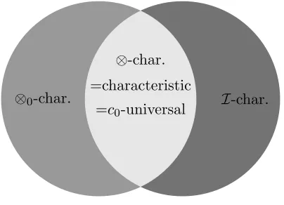
⊗-char.

=characteristic

=c0-universal

I-char.

⊗0-char.

Figure 3: Simplification of theF-ispd property of tensor product kernels; see Remark 7.

which is strictly positive definite (m= 2,3). However,⊗3

m=1km is notI-characteristic. See

Section 5.7 for details.

Remark 7 Note that the l.h.s. in (7) is positive if and only if each term on the r.h.s. is positive, i.e., if k=⊗M

m=1km is ⊗-characteristic with km-s beingc0-kernels on LCP Xm-s,

then all km-s are c0-universal. A similar result was also proved by Steinwart and Ziegel

(2017, Lemma 3.4). Combining this with Theorem 5 yields that for tensor product c0

-kernels, the notions of ⊗-characteristic, characteristic and c0-universality are equivalent, which is quite surprising as for a joint kernel k (that is not of product type), these notions need not necessarily coincide. In light of this discussion, Figure 2(a) can be simplified to Figure 3.

5. Proofs

In this section, we provide the proofs of our results presented in Section 4.

5.1 Proof of Remark 2(iv)

By the second-countability ofXm-s,B ×Mm=1Xm

=⊗M

m=1B(Xm), where the r.h.s. is defined

as the σ-field generated by the cylinder sets Am ×n6=m Xn where m ∈ [M] and Am ∈

B(Xm). Suppose there exists F ∈ ⊗Mm=1Mb(Xm) 0

∩ I such that F 6= 0. This means there exists P ∈ M+1 ×Mm=1Xm

with (Pm)Mm=1 being the marginals of P such that F =

⊗M

m=1Fm = P− ⊗Mm=1Pm. Since F 6= 0 there exists Am×n6=m Xn for some m ∈ [M] and

Am ∈B(Xm) such that 06=F(Am×n6=mXn) =Fm(Am)Qn6=mFn(Xn) =P(Am×n6=mXn)−

Pm(Am)Q_n6=mPn(Xn) =Pm(Am)−Pm(Am) = 0, leading to a contradiction.

5.2 Proof of Example 1

The proof is structured as follows.

2. Next it is proved that k1 ⊗k2 is not ⊗-characteristic, which implies k1 ⊗k2 is not characteristic.

3. Finally, theI-characteristic property of k1⊗k2 is established. The individual steps are as follows:

k is a kernel. Assume w.l.o.g. thatx1 =. . . =xN = 1, xN+1 =. . .=xn= 2. Then it is

easy to verify that the Gram matrix G= [k(xi, xj)]n_i,j=1 =aa> where a:= 1>_N,−1>_n−N >

and a> is the transpose of a. Clearly Gis positive semidefinite and sokis a kernel. k is characteristic. We will show that k satisfies (5). On X = {1,2} a finite signed measure Ftakes the form F=a1δ1+a2δ2 for somea1, a2 ∈R. Thus,

F∈Mb(X)\{0} ⇔(a1, a2)6=0 and F(X) = 0⇔a1+a2 = 0. (9) Consider

Z

X

Z

Xk(x, x 0_{) d}

F(x) dF(x0) =a21k(1,1) +a22k(2,2) + 2a1a2k(1,2)

=a2₁+a2₂−2a1a2= (a1−a2)2 = 4a2₁>0, (10) where we used (9) and the facts thatk(1,1) =k(2,2) = 1, k(1,2) =−1.

k1⊗k2 is not⊗-characteristic. We construct a witnessF=F1⊗F2∈ ⊗2m=1Mb(Xm)\{0}

such that

F(X1×X2) =F1(X1)F2(X2) = 0, (11)

and

0 =

Z

X1×X2

Z

X1×X2

(k1⊗k2)((i1, i2),(i0₁, i0₂))

| {z }

k1(i1,i01)k2(i2,i02)

dF(i1, i2) dF(i01, i02)

= 2

Y

m=1

Z

Xm

Z

Xm

km(im, i0m) dFm(im) dFm(i0m). (12)

Finite signed measures on {1,2} take the form F1 = F1(a) = a1δ1+a2δ2, F2 = F2(b) = b1δ1+b2δ2form, wherea= (a1, a2)∈R2,b= (b1, b2)∈R2. With these notations, (11) and (12) can be rewritten as

0 = (a1+a2)(b1+b2),

0 =





2

X

i,i0₌₁

k1(i, i0)aiai0



 



2

X

j,j0₌₁

k2(j, j0)bjbj0



= (a1−a2)2(b1−b2)2.

Keeping the solutions where neither a nor b is the zero vector, there are 2 (symmetric) possibilities: (i) a1+a2 = 0, b1 =b2 and (ii)a1 =a2,b1+b2 = 0. In other words, for any a, b6= 0, the possibilities are (i)a= (a,−a),b= (b, b) and (ii)a= (a, a),b= (b,−b). This establishes the non-⊗2

m=1Mb(Xm) 0

k1⊗k2 is I-characteristic. Our goal is to show that k1 ⊗k2 is I-characteristic, i.e., for any P∈M+1(X1×X2), µk1⊗k2(F) = 0 impliesF= 0, whereF=P−P1⊗P2. We divide the

proof into two parts:

1. First we derive the equations of

F(X1×X2) = 0 and

Z Z

(X1×X2)2

(k1⊗k2) ((i, j),(r, s)) dF(i, j) dF(r, s) = 0 (13)

for general finite signed measures F=P2i,j=1aijδ(i,j) onX1×X2.

2. Then, we apply theF=P−P1⊗P2parameterization and solve forPthat satisfies (13) to conclude thatP=P1⊗P2, i.e.,F= 0. Note that in the chosen parametrization for F,F(X1×X2) = 0 holds automatically.

The details are as follows.

Step 1.

0 =F(X1×X2)⇔0 =a11+a12+a21+a22, (14)

0 =

Z

X1×X2

Z

X1×X2

(k1⊗k2) ((i, j),(r, s))

| {z }

k1(i,r)k2(j,s)

dF(i, j) dF(r, s)

= 2

X

i,j=1 2

X

r,s=1

k1(i, r)k2(j, s)aijars=

2

X

i,r=1

k1(i, r) 2

X

j,s=1

k2(j, s)aijars

=k1(1,1) [k2(1,1)a11a11+k2(1,2)a11a12+k2(2,1)a12a11+k2(2,2)a12a12] +k1(1,2) [k2(1,1)a11a21+k2(1,2)a11a22+k2(2,1)a12a21+k2(2,2)a12a22] +k1(2,1) [k2(1,1)a21a11+k2(1,2)a21a12+k2(2,1)a22a11+k2(2,2)a22a12] +k1(2,2) [k2(1,1)a21a21+k2(1,2)a21a22+k2(2,1)a22a21+k2(2,2)a22a22] = a2₁₁−2a11a12+a212

| {z }

(a11−a12)2

+ a2₂₁−2a21a22+a222

| {z }

(a21−a22)2

−2 (a11a21−a11a22−a12a21+a12a22)

| {z }

(a11−a12)(a21−a22)

= (a11−a12−a21+a22)2. (15)

Solving (14) and (15) yields

a11+a22= 0 and a12+a21= 0. (16)

Step 2. AnyP∈M+1(X1×X2) can be parametrized as

P= 2

X

i,j=1

pijδ(i,j), pij ≥0,∀(i, j) and

2

X

i,j=1

pij = 1. (17)

LetF=P−P1⊗P2 =P2i,j=1aijδ(i,j); for illustration see Table 1. It follows from step 1 that Fsatisfying (16) is equivalent to satisfying (13). Therefore, for the choice ofF:=P−P1⊗P2, we obtain

P: y\x 1 2 P2

1 p11 p21 q1=p11+p21

2 p12 p22 q2=p12+p22

P1 p1=p11+p12 p2 =p21+p22

⇒

F:=P−P1⊗P2 1 2

1 a11=p11−(p11+p12)(p11+p21) a21=p21−(p21+p22)(p11+p21) 2 a12=p12−(p11+p12)(p12+p22) a22=p22−(p21+p22)(p12+p22)

Table 1: Joint (P), joint minus product of the marginals (P−P1⊗P2).

P: y\x 1 2 P2

1 p11= a[1 −(a+b)]

a+b p21=a q1=

a a+b

2 p12= b[1−_a(₊a_b+b)] p22=b q2= _a+b_b P1 p1 = 1−(a+b) p2=a+b

Table 2: Family of probability distributions solving (17)–(19).

p12−(p11+p12)(p12+p22) +p21−(p21+p22)(p11+p21) = 0, (19) where (pij)i,j∈[2] satisfy (17). Solving (17)–(19), we obtain

p11=

a[1−(a+b)]

a+b , p12=

b[1−(a+b)]

a+b , p21=a and p22=b,

with 0 ≤ a, b ≤ 1, a+b ≤ 1 and (a, b) 6= 0. The resulting distribution family with its marginals is summarized in Table 2. It can be seen that each member of this family (any a,b in the constraint set) factorizes: P = P1⊗P2. In other words, F =P−P1⊗P2 = 0; hencek1⊗k2 is I-characteristic.

Remark. We would like to mention that while k1 and k2 are characteristic, they are not universal. Since Xis finite, the usual notion of universality (also called c-universality) matches with c0-universality. Therefore, from (10), we have R_XR_Xk(x, x0) dF(x) dF(x) = (a1−a2)2 where F =a1δ1+a2δ2 for some a1, a2 ∈ R\{0}. Clearly, the choice of a1 =a2 establishes that there existsF∈Mb(X)\{0}such that

R

X

R

Xk(x, x0) dF(x) dF(x) = 0. Hence kis not universal. Note that the constraint in (9), which is needed to verify the characteristic property of kis not needed to verify its universality.

(i) Supposek1 and k2 are characteristic and that for someF=P−P1⊗P2 ∈ I, H1⊗H2 3

Z

X1×X2

(k1⊗k2) (·, x) dF(x) =

Z

X1×X2

k1(·, x1)⊗k2(·, x2) dF(x) = 0, (20) where x = (x1, x2). We want to show that F = 0. By the second-countability of Xm-s,

the product σ-field, i.e., ⊗2

m=1B(Xm) generated by the cylinder sets B1×X2 and X1×B2

(Bm∈B(Xm), m= 1,2), coincides with the Borelσ-field B(X1×X2) on the product space

(Dudley, 2004, Lemma 4.1.7):

⊗2_m=1B(Xm) =B(X1×X2).

Hence, it is sufficient to prove thatF(B1×B2) = 0,∀Bm∈B(Xm),m= 1,2. To this end,

it follows from (20) that for all h2 ∈H2, H1 3

Z

X1×X2

k1(·, x1)h2(x2) dF(x) =

Z

X1

k1(·, x1) dν(x1) = 0, (21) where

ν(B1) :=νh2(B1) =

Z

X1×X2

χB1(x1)h2(x2) dF(x), B1 ∈B(X1).

Since k1 is characteristic, (21) implies ν = 0, provided that |ν|(X1) < ∞ and ν(X1) = 0. These two requirements hold:

ν(X1) =

Z

X1×X2

h2(x2) dF(x) =

Z

X2

h2(x2) d[P2−P2](x2) = 0,

|ν|(X1)≤

Z

X1×X2

|h2(x2)|

| {z }

hh2,k2(·,x2)i_H 2

d[P+P1⊗P2](x1, x2)

≤ kh2k_H2

Z

X1×X2

p

k2(x2, x2) d[P+P1⊗P2](x1, x2)

≤2kh2k_H2

Z

X2

p

k2(x2, x2) dP2(x2)<∞,

where the last inequality follows from the boundedness ofk2. The establishedν = 0 implies that for∀B1∈B(X1) and ∀h2 ∈H2,

0 =ν(B1) =

h2,

Z

X1×X2

χB1(x1)k2(·, x2) dF(x)

H2

,

and hence

0 =

Z

X1×X2

χB1(x1)k2(·, x2) dF(x) =

Z

X2

k2(·, x2) dθB1(x2), (22)

where

θB1(B2) =

Z

X1×X2

Using the characteristic property of k2, it follows from (22) that θB1 = 0 for ∀B1 ∈B(X1),

i.e.,

0 =θB1(B2) =F(B1×B2), ∀B1∈B(X1),∀B2 ∈B(X2)

provided that θB1(X2) = 0 and |θB1|(X2)<∞. Indeed, both these conditions hold:

θB1(X2) =

Z

X1×X2

χB1(x1) dF(x) =

Z

X1

χB1(x1) d[P1−P1](x1) = 0,

|θB1|(X2)≤

Z

X1×X2

d[P+P1⊗P2](x) = 2.

(ii) Assume w.l.o.g. thatk1is not characteristic. This means there existsP16=P01∈M+1(X1) such thatµk1(P1) =µk1(P

0

1). Our goal is to construct an F∈M+1 ×Mm=1Xm

such that

µ_⊗M

m=1km F− ⊗

M m=1Fm

=

Z

×M m=1

⊗M_m=1km(·, xm) d

F− ⊗Mm=1Fm

= 0, butF6=⊗Mm=1Fm.

Define I:=F− ⊗Mm=1Fm ∈ I. In other words we want to get a witnessI∈ I proving that

⊗M

m=1km is not I-characteristic. Let us take z=6 z0 ∈X2, which is possible since|X2| ≥2.

Let us define Fas6

F= P1⊗δz⊗(⊗

M

m=3Qm) +P01⊗δz0⊗(⊗M

m=3Qm)

2 ∈M

+

1 ×Mm=1Xm

.

It is easy to verify that

F1= P1+P 0 1 2 ,F2 =

δz+δz0

2 and Fm =Qm (m= 3, . . . , M),

whereQ3, . . . ,QM are arbitrary probability measures onX3, . . . ,XM, respectively. First we

check that I6= 0. Indeed it is the case since

• z6=z0 andX2is a Hausdorff space, there existsB2∈B(X2) such thatz∈B2,z06∈B2.

• _P1 6=P01,P1(B1)=6 P01(B1) for some B1 ∈B(X1). LetS =B1×B2× ×M

m=3Xm

, and compare its measure underF and⊗Mm=1Fm:

F(S) = P1(B1)

=1 (z∈B2)

z }| {

δz(B2) QMm=3 =1

z }| {

Qm(Xm) +P01(B1)

=0 (z0_6∈B 2)

z }| {

δz0(B₂) QM

m=3 =1

z }| {

Qm(Xm)

2

= P1(B1) 2 ,

⊗M_m=1Fm

(S) =

M Y

m=1

Fm(Bm) =

P1(B1) +P01(B1) 2

=1

z }| {

δz(B2) +

=0

z }| {

δz0(B2)

2

M Y

m=3 =1

z }| {

Qm(Xm)

6. TheFconstruction specializes to that of Lyons (2013, Proposition 3.15) in theM = 2 case; Lyons used

= P1(B1) +P 0 1(B1)

4 6=

P1(B1) 2 ,

where the last equality holds sinceP1(B1)6=P01(B1). This shows thatI=F− ⊗Mm=1Fm 6= 0

sinceI(S)6= 0.

Next we prove that µ_⊗M

m=1km F− ⊗

M m=1Fm

= 0. Indeed,

µ_⊗M

m=1km(I) =

Z

×M m=1Xm

⊗M_m=1km(·, xm) d

F− ⊗Mm=1Fm

(x1, . . . , xM)

=

Z

×M m=1Xm

⊗M

m=1km(·, xm) d

P1⊗δz+P01⊗δz0

2 −

P1+P01

2 ⊗

δz+δz0

2

⊗ ⊗M_m=3Qm

(x1, . . . , xM)

=

Z

×M m=1Xm

⊗M

m=1km(·, xm) d

P1(x1)⊗δz(x2) +P01(x1)⊗δz0(x₂)

2

−P1(x1)⊗δz(x2) +P1(x1)⊗δz0(x2)

4

−P

0

1(x1)⊗δz(x2) +P01(x1)⊗δz0(x₂)

4

⊗(⊗M

m=3Qm(xm))

(∗) =

µk1(P1)⊗k2(·, z) +µk1(P

0

1)⊗k2(·, z0) 2

−µk1(P1)⊗k2(·, z) +µk1(P1)⊗k2(·, z

0₎

4

−µk1(P

0

1)⊗k2(·, z) +µk1(P

0

1)⊗k2(·, z0) 4

⊗

⊗M_m=3µkm(Qm)

= 0

|{z}

∈Hk₁⊗k₂ ⊗

⊗M_m=3µkm(Qm)

= 0,

where we used µk1(P1) =µk1(P

0

1) in (∗). 5.4 Proof of Example 2

LetM = 3, ×M

m=1Xm ={(i1, i2, i3) :im ∈ {1,2}, m ∈[3]},km(x, x0) = 2δx,x0−1. Our goal

is to show that⊗3

m=1km is not I-characteristic. The structure of the proof is as follows:

1. First we describe the equations of the non-characteristic property of ⊗3

m=1km with

a general finite signed measure F = P2i1,i2,i3=1ai1,i2,i3δ(i1,i2,i3) on ×

3

m=1Xm where

ai1,i2,i3 ∈R(∀i1, i2, i3).

2. Next, we apply the F=P− ⊗3m=1Pm parameterization and show that there exists P that satisfies the equations of step 1 to conclude that⊗3

m=1km is notI-characteristic.

The details are as follows.

Step 1. The equations of non-characteristic property in terms ofA= [ai1,i2,i3](im)3m=1∈[2]3 ∈

R2×2×2 are

F∈Mb ×3m=1Xm

0 =F(×3_m=1Xm)⇔0 =

2

X

i1,i2,i3=1

ai1,i2,i3, (23)

0 =

Z

×3 m=1Xm

Z

×3 m=1Xm

(⊗3_m=1km) (i1, i2, i3),(i01, i 0 2, i

0 3)

| {z }

Q3

m=1km(im,i0m)

dF(i1, i2, i3) dF(i0₁, i0₂, i0₃)

= 2

X

i1,i2,i3=1

2

X

i0₁,i0₂,i0₃=1 3

Y

m=1

km(im, i0m)ai1,i2,i3ai0₁,i0₂,i0₃. (24)

Solving (23) and (24) yields

a1,1,1+a1,2,2+a2,1,2+a2,2,1 = 0 and a1,1,2+a1,2,1+a2,1,1+a2,2,2 = 0.

Step 2. The equations of non I-characteristic property can be obtained from step 1 by choosingF=P− ⊗Mm=1Pm, where

P= 2

X

i1,i2,i3=1

pi1,i2,i3δ(i1,i2,i3) and P= [pi1,i2,i3](im)3m=1∈[2]3 ∈R

2×2×2_.

In other words, it is sufficient to obtain a P that solves the following system of equations for which A=A(P)6=0:

2

X

i1,i2,i3=1

pi1,i2,i3 = 1, (25)

pi1,i2,i3 ≥0,∀(i1, i2, i3)∈[2]

3_{, (26)}

a1,1,1+a1,2,2+a2,1,2+a2,2,1= 0, (27) a1,1,2+a1,2,1+a2,1,1+a2,2,2= 0, (28) where

ai1,i2,i3 =pi1,i2,i3 −p1,i1p2,i2p3,i3, (29)

and

p1,i1 =

2

X

i2,i3=1

pi1,i2,i3, p2,i2 =

2

X

i1,i3=1

pi1,i2,i3, p3,i3 =

2

X

i1,i2=1

pi1,i2,i3. (30)

One can get an analytical description for the solution of (25)–(30), where the solutionP(z) is parameterized by z = (z0, . . . , z5)∈ _R6_{. For explicit expressions, we refer the reader to} Appendix A. In the following, we present two examples of P that satisfy (25)–(30) such thatA6=0, thereby establishing the nonI-characteristic property of ⊗3

m=1km.

1. P:

p1,1,1= 1

5, p1,1,2 = 1

10, p1,2,1 = 1

10, p1,2,2= 1 10, p2,1,1=

1

5, p2,1,2 = 1

10, p2,2,1 = 1

and A:

a1,1,1 = 1

50, a1,1,2 =− 1

50, a1,2,1=− 1

50, a1,2,2 = 1

50, (31) a2,1,1 =

1

50, a2,1,2 =− 1

50, a2,2,1=− 1

50, a2,2,2 = 1

50. (32)

2. P:

p1,1,1 = 0, p1,1,2 = 1

10, p1,2,1= 1

10, p1,2,2 = 1 10, p2,1,1 =

1

10, p2,1,2 = 1

10, p2,2,1= 3

10, p2,2,2 = 1 5, and A:

a1,1,1=− 9

200, a1,1,2= 11

200, a1,2,1 =− 1

200, a1,2,2 =− 1 200, a2,1,1=−

1

200, a2,1,2=− 1

200, a2,2,1 = 11

200, a2,2,2 =− 9 200.

In fact these examples are obtained with the choices z = (₁₀1 ,₁₀1,₁₀1 ,₁₀1,₁₀1 ,₁₀1) and z = (₁₀3 ,₁₀1,₁₀1 ,₁₀1,₁₀1,₁₀2) respectively. See Appendix A for details.

5.5 Proof of Theorem 4

It follows from (8) and Remark 2(iii) that (v)⇒(iii)⇒(ii)⇔(i). It also follows from (8) and Theorem 3(ii) that (v) ⇒ (iv) ⇒ (i). We now show that (i) ⇒ (v) which establishes the equivalence of (i)–(v). Suppose (i) holds. Then by Bochner’s theorem (Wendland, 2005, Theorem 6.6), we have that for allm∈[M],

km(xm, ym) = Z

Rdm

e− √

−1hωm,xm−ymi_dΛ

m(ωm), xm, ym ∈Rdm,

where (Λm)Mm=1 are finite non-negative Borel measures on (Rdm)Mm=1 respectively. This implies

⊗M_m=1km(xm, ym) =⊗Mm=1

Z

Rdm

e− √

−1hωm,xm−ymi_dΛ

m(ωm) = Z

Rd

e− √

−1hω,x−yi_dΛ(ω),

where x = (x1, . . . , xM) ∈ Rd, y = (y1, . . . , yM) ∈ Rd, ω = (ω1, . . . , ωM) ∈ Rd, d =

PM

m=1dm and Λ := ⊗Mm=1Λm. Sriperumbudur et al. (2010, Theorem 9) showed that km

is characteristic iff supp (Λm) = Rdm, where supp(·) denotes the support of its argument. Since supp(Λ) = supp ⊗M

m=1Λm

= ×M

m=1supp (Λm) = ×Mm=1Rdm = Rd, it follows that

⊗M

m=1km is characteristic.

5.6 Proof of Theorem 5

The c0-kernel property of km-s (m = 1, . . . , M) implies that of ⊗Mm=1km. Moreover, Xm-s

are LCP spaces, hence×M

(⇐) Assume that⊗M

m=1km isc0-universal. Since⊗Mm=1Mb(Xm)⊆Mb ×Mm=1Xm

, we have that for allF=⊗Mm=1Fm ∈ ⊗mM=1Mb(Xm)\{0},

0<

Z

×M m=1Xm

Z

×M m=1Xm

⊗M_m=1km

(x, x0)

| {z }

QM

m=1km(xm,x0m)

dF(x) dF(x0)

=

M Y

m=1

Z

Xm×Xm

km(xm, x0m) dFm(xm) dFm x0m

,

wherex= (x1, . . . , xM) and x0 = (x01, . . . , x0M). The above inequality implies Z

Xm×Xm

km(xm, x0m) dFm(xm) dFm x0m

>0, ∀m∈[M].

Since F∈ ⊗Mm=1Mb(Xm)\{0} iff Fm∈Mb(Xm)\{0}for all m∈[M], the result follows.

(⇒) Assume that km-s are c0-universal. By the note above ⊗Mm=1km is c0-kernel; its c0

-universality is equivalent to the injectivity of µ = µ_⊗M

m=1km on Mb ×

M m=1Xm

. In other words, we want to prove that µ(F) = 0 implies F = 0, whereF ∈Mb ×Mm=1Xm

. We will use the shorthand Hm =Hkm below.

Suppose there exists F∈Mb ×Mm=1Xm

such that

µ_F =

Z

×M m=1Xm

⊗M_m=1km

(·, x)

| {z }

⊗M

m=1km(·,xm)

dF(x) = 0 (∈ ⊗M_m=1Hm). (33)

Since Xm-s are LCP, ⊗Mm=1B(Xm) = B ×Mm=1Xm

(Steinwart and Christmann, 2008, page 480). Hence, in order to getF= 0 it is sufficient to prove that

F ×Mm=1Bm

= 0, ∀Bm∈B(Xm), m∈[M].

We will prove by induction that form= 0, . . . , M

⊗M_j=m+1H_j 3

0 =

Z

×M j=1Xj

m Y

j=1

χBj(xj)⊗

M

j=m+1kj(·, xj) dF(x)

=:o(B1, . . . , Bm, km+1, . . . , kM),∀Bj ∈B(Xj), j∈[m], (34)

which

(∗) reduces to (33) when m= 0 by defining Q0

j=1χBj(xj) := 1;

(†) for m =M,⊗M

m=M+1Hm is defined to be equal to R and ⊗mM=M+1km(·, xm) := 1, in

which caseo(B1, . . . , BM) =F

×M j=1Bj

= 0⇒F= 0, the result we want to prove.

From the above, it is clear that (34) holds for m = 0. Assuming (34) holds for some m, we now prove that it holds for m+ 1. To this end, it follows from (34) that ∀hm+2 ∈ Hm+2, . . . ,∀hM ∈HM,

=



 Z

×M j=1Xj



 m Y

j=1

χBj(xj)



⊗M_j=m+1kj(·, xj) dF(x)



(hm+2, . . . , hM)

=

Z

×M j=1Xj

km+1(·, xm+1)

m Y

j=1

χBj(xj)

M Y

j=m+2

hj(xj) dF(x)

=

Z

Xm+1

km+1(·, xm+1) dν(xm+1),

where

ν(B) :=νB1,...,Bm,hm+2,...,hM(B)

=

Z

×M j=1Xj



 m Y

j=1

χBj(xj)



χ_B(xm+1) 

 M Y

j=m+2 hj(xj)



dF(x), B∈B(Xm+1).

By the c0-universality ofkm+1,

ν = 0 for∀hm+2∈Hm+2, . . . ,∀hM ∈HM (35)

provided that ν∈Mb(Xm+1), in other words if |ν|(Xm+1)<∞. This condition is met:

|ν|(Xm+1)≤ Z

×M j=1Xj

M Y

j=m+2

hhj, kj(·, xj)iHj

| {z }

≤khjk_H j

√

kj(xj,xj)

d|F|(x)

≤ |_F| ×M_m=1Xm

M Y

j=m+2

khjk_Hj sup x∈Xj,x0∈Xj

q

kj(x, x0)<∞,

where we used the boundedness ofkm-s in the last inequality. (35) implies that for∀B1 ∈

B(X1), . . . ,∀Bm+1∈B(Xm+1) and∀hm+2∈Hm+2, . . . ,∀hM ∈HM

0 =ν(Bm+1) =

Z

×M j=1Xj



 m+1

Y

j=1

χBj(xj)

    M Y

j=m+2 hj(xj)



 dF(x)

=

*

⊗M_j=m+2hj, Z

×M j=1Xj



 m+1

Y

j=1

χBj(xj)



⊗M_j=m+2k_j(·, x_j) dF(x) +

⊗M j=m+2Hj

,

and therefore

o(B1, . . . , Bm+1, km+2, . . . , kM) = Z

×M j=1Xj



 m+1

Y

j=1

χBj(xj)



⊗M_j=m+2k(·, xj) dF(x) = 0 ∈ ⊗M_j=m+2Hj

for∀B1∈B(X1), . . . ,∀Bm+1∈B(Xm+1), i.e., (34) holds form+1. Therefore, by induction, (34) holds for m = M and the result follows from (†). To justify the convention in (†), consider the case ofm=M −1 in which case (34) can be written as

Z

XM

kM(·, xM) dν(xM) = 0,

where

ν(B) =

Z

×M j=1Xj



 M−1

Y

j=1

χBj(xj)



χB(xM) dF(x), B ∈B(XM).

Then by the c0-universal property ofkM, since

|ν|(XM)≤ Z

×M j=1Xj

1 d|_F|(x) =|_F| ×M_j=1Xj

<∞

we obtain

Z

×M j=1Xj

M Y

j=1

χBj(xj) dF(x) =F ×

M j=1Bj

= 0,∀B1 ∈B(X1), . . . ,∀BM ∈B(XM).

5.7 Proof of Example 3

The proof follows by a simple modification of that of Example 2 (Section 5.4). The equations of a witness A= [ai1,i2,i3](im)3m=1∈[2]3 (and corresponding P= [pi1,i2,i3](im)3m=1∈[2]3) for the

non-I-characteristic property of ⊗3

m=1km take the form:

A6=0,

0 = 2

X

i1,i2,i3=1

ai1,i2,i3, (36)

0 = 2

X

i1,i2,i3=1

2

X

i0 1,i02,i03=1

3

Y

m=1

km(im, i0m)ai1,i2,i3ai0₁,i0₂,i0₃

= (a1,1,1−a2,1,1)2+ (a1,1,2−a2,1,2)2+ (a1,2,1−a2,2,1)2+ (a1,2,2−a2,2,2)2, (37)

where (36) and (37) are equivalent to

0 = 2

X

i1,i2,i3=1

ai1,i2,i3, a1,1,1 =a2,1,1, a1,1,2=a2,1,2, a1,2,1 =a2,2,1, a1,2,2 =a2,2,2. (38)

While (38) is more restrictive than (27) and (28) (hence its solution set might even be empty), one can immediately see that the example of A6=0 given in (31) and (32) fulfills (38) proving the non-I-characteristic property of⊗3

Acknowledgments

The authors profusely thank Ingo Steinwart for fascinating discussions on topics related to the paper and for contributing to Remark 7. The authors also thank the anonymous reviewers for their constructive comments that improved the manuscript. A part of the work was carried out while BKS was visiting ZSz at CMAP, ´Ecole Polytechnique. BKS is supported by NSF-DMS-1713011 and also thanks CMAP and DSI for their generous support. ZSz is highly grateful for the Greek hospitality around the Aegean Sea; it greatly contributed to the development of the induction arguments.

Appendix A. Analytical Solution to (25)–(30) in Example 2

The solution of (25)–(30) takes the form

p1,1,1=−

z2+z1+z4+z5−3z2z1−4z2z4−4z1z4−z2z3−2z2z0−2z1z3−3z2z5

−2z4z3−z1z0−3z1z5−2z4z0−4z4z5−z3z0−z3z5−z0z5+ 2z2z₁2+ 2z2₂z1 + 4z2z42+ 2z22z4+ 4z1z24+ 2z12z4+ 2z22z0+ 2z12z3+ 2z2z52+ 2z22z5+ 2z42z3 + 2z1z₅2+ 2z2₁z5+ 2z₄2z0+ 2z4z₅2+ 4z2₄z5−z₂2−z₁2−3z₄2+ 2z₄3−z₅2 + 6z2z1z4+ 2z2z1z3+ 2z2z4z3+ 2z2z1z0+ 4z2z1z5+ 4z2z4z0+ 4z1z4z3 + 6z2z4z5+ 2z1z4z0+ 6z1z4z5+ 2z2z3z0+ 2z2z3z5+ 2z1z3z0+ 2z2z0z5 + 2z1z3z5+ 2z4z3z0+ 2z4z3z5+ 2z1z0z5+ 2z4z0z5

2z2z1−z1−2z4−z3−z0−2z5−z2+ 2z2z4+ 2z1z4+ 2z2z0+ 2z1z3+ 2z2z5 + 2z4z3+ 2z1z5+ 2z4z0+ 4z4z5+ 2z3z0+ 2z3z5+ 2z0z5+ 2z₄2+ 2z₅2

,

p1,1,2=z2, p1,2,1=z1, p1,2,2=z4,

p2,1,1=−

z4+z3+z0+z5−z2z1−z2z4−z1z4−z2z3−2z2z0−2z1z3−2z2z5

−3z4z3−z1z0−2z1z5−3z4z0−4z4z5−3z3z0−4z3z5−4z0z5+ 2z2z20 + 2z1z₃2+ 2z2z₅2+ 2z4z2₃+ 2z₄2z3+ 2z1z₅2+ 2z4z2₀+ 2z₄2z0+ 4z4z₅2+ 2z₄2z5 + 2z3z02+ 2z23z0+ 4z3z25+ 2z32z5+ 4z0z52+ 2z02z5−z42−z32−z02−3z52 + 2z₅3+ 2z2z1z3+ 2z2z4z3+ 2z2z1z0+ 2z2z1z5+ 2z2z4z0+ 2z1z4z3 + 2z2z4z5+ 2z1z4z0+ 2z1z4z5+ 2z2z3z0+ 2z2z3z5+ 2z1z3z0+ 4z2z0z5 + 4z1z3z5+ 4z4z3z0+ 6z4z3z5+ 2z1z0z5+ 6z4z0z5+ 6z3z0z5

2z2z1−z1−2z4−z3−z0−2z5−z2+ 2z2z4+ 2z1z4+ 2z2z0+ 2z1z3+ 2z2z5 + 2z4z3+ 2z1z5+ 2z4z0+ 4z4z5+ 2z3z0+ 2z3z5+ 2z0z5+ 2z₄2+ 2z₅2

,

form, where z= (z0, z1, . . . , z5)∈R6 satisfies

0≤(2z0z2−z1−z2−z3−2z4−2z5−z0+ 2z0z3+ 2z1z2+ 2z0z4+ 2z1z3+ 2z0z5 +2z1z4+ 2z1z5+ 2z2z4+ 2z2z5+ 2z3z4+ 2z3z5+ 4z4z5+ 2z₄2+ 2z₅2×

(z0z3−z3−z4−z5−z0z1−z0−z1z2+z0z5−2z1z4−z2z3−z1z5−2z2z4−z2z5 +z3z5+ 2z0z22+ 2z1z22+ 2z12z2+ 2z0z42+ 2z12z3+ 4z1z42+ 2z12z4+ 2z1z52+ 4z2z42 +2z₁2z5+ 2z₂2z4+ 2z2z₅2+ 2z3z₄2+ 2z₂2z5+ 2z4z₅2+ 4z₄2z5−z₁2−z2₂−z₄2+ 2z3₄+z₅2 +2z0z1z2+ 2z0z1z3+ 2z0z1z4+ 2z0z2z3+ 2z0z1z5+ 4z0z2z4+ 2z1z2z3+ 2z0z2z5 +2z0z3z4+ 6z1z2z4+ 4z1z2z5+ 4z1z3z4+ 2z0z4z5+ 2z1z3z5+ 2z2z3z4+ 6z1z4z5 +2z2z3z5+ 6z2z4z5+ 2z3z4z5),

0≤(2z0z2−z1−z2−z3−2z4−2z5−z0+ 2z0z3+ 2z1z2+ 2z0z4+ 2z1z3+ 2z0z5 +2z1z4+ 2z1z5+ 2z2z4+ 2z2z5+ 2z3z4+ 2z3z5+ 4z4z5+ 2z42+ 2z52

×

(z1z2−z2−z4−z5−z0z1−z0z3−z1−z0z4−2z0z5+z1z4−z2z3+z2z4

−z3z4−2z3z5+ 2z₀2z2+ 2z0z₃2+ 2z₀2z3+ 2z0z₄2+ 2z1z₃2+ 2z2₀z4+ 4z0z2₅+ 2z₀2z5 +2z1z52+ 2z2z52+ 2z3z42+ 2z32z4+ 4z3z52+ 2z23z5+ 4z4z25+ 2z42z5−z02−z32+z42

−z₅2+ 2z3₅+ 2z0z1z2+ 2z0z1z3+ 2z0z1z4+ 2z0z2z3+ 2z0z1z5+ 2z0z2z4+ 2z1z2z3 +4z0z2z5+ 4z0z3z4+ 6z0z3z5+ 2z1z2z5+ 2z1z3z4+ 6z0z4z5+ 4z1z3z5+ 2z2z3z4 +2z1z4z5+ 2z2z3z5+ 2z2z4z5+ 6z3z4z5),

2z0z2+ 2z0z3+ 2z1z2+ 2z0z4+ 2z1z3+ 2z0z5+ 2z1z4+ 2z1z5+ 2z2z4+ 2z2z5

+ 2z3z4+ 2z3z5+ 4z4z5+ 2z24+ 2z52 6=z0+z1+z2+z3+ 2z4+ 2z5,

(2z0z2−z1−z2−z3−2z4−2z5−z0+ 2z0z3+ 2z1z2+ 2z0z4+ 2z1z3+ 2z0z5 +2z1z4+ 2z1z5+ 2z2z4+ 2z2z5+ 2z3z4+ 2z3z5+ 4z4z5+ 2z₄2+ 2z₅2×

(z1+z2+z4+z5−z0z1−2z0z2−z0z3−3z1z2−2z0z4−2z1z3−z0z5−4z1z4

−z2z3−3z1z5−4z2z4−3z2z5−2z3z4−z3z5−4z4z5+ 2z0z2₂+ 2z1z₂2+ 2z2₁z2 +2z0z42+ 2z12z3+ 4z1z42+ 2z12z4+ 2z1z52+ 4z2z42+ 2z12z5+ 2z22z4+ 2z2z52 +2z3z42+ 2z22z5+ 2z4z52+ 4z42z5−z12−z22−3z42+ 2z43−z52+ 2z0z1z2 +2z0z1z3+ 2z0z1z4+ 2z0z2z3+ 2z0z1z5+ 4z0z2z4+ 2z1z2z3+ 2z0z2z5

+2z0z3z4+ 6z1z2z4+ 4z1z2z5+ 4z1z3z4+ 2z0z4z5+ 2z1z3z5+ 2z2z3z4+ 6z1z4z5 + 2z2z3z5+ 6z2z4z5+ 2z3z4z5)≤0,

(2z0z2−z1−z2−z3−2z4−2z5−z0+ 2z0z3+ 2z1z2+ 2z0z4+ 2z1z3+ 2z0z5 +2z1z4+ 2z1z5+ 2z2z4+ 2z2z5+ 2z3z4+ 2z3z5+ 4z4z5+ 2z₄2+ 2z₅2×

(z0+z3+z4+z5−z0z1−2z0z2−3z0z3−z1z2−3z0z4−2z1z3−4z0z5

+2z0z32+ 2z02z3+ 2z0z42+ 2z1z32+ 2z02z4+ 4z0z52+ 2z02z5+ 2z1z52+ 2z2z52 +2z3z₄2+ 2z₃2z4+ 4z3z₅2+ 2z₃2z5+ 4z4z₅2+ 2z₄2z5−z₀2−z₃2−z2₄−3z₅2+ 2z₅3 +2z0z1z2+ 2z0z1z3+ 2z0z1z4+ 2z0z2z3+ 2z0z1z5+ 2z0z2z4+ 2z1z2z3 +4z0z2z5+ 4z0z3z4+ 6z0z3z5+ 2z1z2z5+ 2z1z3z4+ 6z0z4z5+ 4z1z3z5 +2z2z3z4+ 2z1z4z5+ 2z2z3z5+ 2z2z4z5+ 6z3z4z5)≤0,

and 0≤z0, z1, z2, z3, z4, z5 ≤1.

The above analytic solution to (25)–(30) is obtained by symbolic math programming in MATLAB.

References

N. Aronszajn. Theory of reproducing kernels. Transactions of the American Mathematical Society, 68:337–404, 1950.

K. Balasubramanian, T. Li, and M. Yuan. On the optimality of kernel-embedding based goodness-of-fit tests. Technical report, 2017. (https://arxiv.org/abs/1709.08148).

L. Baringhaus and C. Franz. On a new multivariate two-sample test.Journal of Multivariate Analysis, 88:190–206, 2004.

A. Berlinet and C. Thomas-Agnan. Reproducing Kernel Hilbert Spaces in Probability and Statistics. Kluwer, 2004.

G. Blanchard, G. Lee, and C. Scott. Generalizing from several related classification tasks to a new unlabeled sample. InAdvances in Neural Information Processing Systems (NIPS), pages 2178–2186, 2011.

G. Blanchard, A. A. Deshmukh, U. Dogan, G. Lee, and C. Scott. Domain generalization by marginal transfer learning. Technical report, 2017. (https://arxiv.org/abs/1711. 07910).

K. Borgwardt, A. Gretton, M. J. Rasch, H.-P. Kriegel, B. Sch¨olkopf, and A. J. Smola. Inte-grating structured biological data by kernel maximum mean discrepancy. Bioinformatics, 22:e49–e57, 2006.

J.-F. Cardoso. Multidimensional independent component analysis. In International Con-ference on Acoustics, Speech, and Signal Processing (ICASSP), pages 1941–1944, 1998.

C. Carmeli, E. De Vito, A. Toigo, and V. Umanit´a. Vector valued reproducing kernel Hilbert spaces and universality. Analysis and Applications, 8:19–61, 2010.

K. Chwialkowski, H. Strathmann, and A. Gretton. A kernel test of goodness of fit. In

International Conference on Machine Learning (ICML; PMLR), volume 48, pages 2606– 2615, 2016.

K. Fukumizu, A. Gretton, X. Sun, and B. Sch¨olkopf. Kernel measures of conditional depen-dence. In Advances in Neural Information Processing Systems (NIPS), pages 498–496, 2008.

K. Fukumizu, F. Bach, and M. Jordan. Kernel dimension reduction in regression. The Annals of Statistics, 37(4):1871–1905, 2009.

K. Fukumizu, L. Song, and A. Gretton. Kernel Bayes’ rule: Bayesian inference with positive definite kernels. Journal of Machine Learning Research, 14:3753–3783, 2013.

A. Gretton. A simpler condition for consistency of a kernel independence test. Technical report, University College London, 2015. (http://arxiv.org/abs/1501.06103).

A. Gretton, O. Bousquet, A. Smola, and B. Sch¨olkopf. Measuring statistical dependence with Hilbert-Schmidt norms. InAlgorithmic Learning Theory (ALT), pages 63–78, 2005a.

A. Gretton, R. Herbrich, A. Smola, O. Bousquet, and B. Sch¨olkopf. Kernel methods for measuring independence. Journal of Machine Learning Research, 6:2075–2129, 2005b.

A. Gretton, K. Fukumizu, C. H. Teo, L. Song, B. Sch¨olkopf, and A. J. Smola. A kernel statistical test of independence. In Advances in Neural Information Processing Systems (NIPS), pages 585–592, 2008.

A. Gretton, K. M. Borgwardt, M. J. Rasch, B. Sch¨olkopf, and A. Smola. A kernel two-sample test. Journal of Machine Learning Research, 13:723–773, 2012.

Z. Harchaoui, F. Bach, and E. Moulines. Testing for homogeneity with kernel Fisher dis-criminant analysis. InAdvances in Neural Information Processing Systems (NIPS), pages 609–616, 2007.

W. Jitkrittum, Z. Szab´o, and A. Gretton. An adaptive test of independence with analytic kernel embeddings. In International Conference on Machine Learning (ICML; PMLR), volume 70, pages 1742–1751, 2017a.

W. Jitkrittum, W. Xu, Z. Szab´o, K. Fukumizu, and A. Gretton. A linear-time kernel goodness-of-fit test. InAdvances in Neural Information Processing Systems (NIPS), pages 261–270, 2017b.

B. Kim, R. Khanna, and O. O. Koyejo. Examples are not enough, learn to criticize! criticism for interpretability. InAdvances in Neural Information Processing Systems (NIPS), pages 2280–2288, 2016.

L. Klebanov. N-Distances and Their Applications. Charles University, Prague, 2005.

G. Kusano, K. Fukumizu, and Y. Hiraoka. Persistence weighted Gaussian kernel for topo-logical data analysis. In International Conference on Machine Learning (ICML), pages 2004–2013, 2016.

Q. Liu, J. Lee, and M. Jordan. A kernelized Stein discrepancy for goodness-of-fit tests. In

International Conference on Machine Learning (ICML), pages 276–284, 2016.

J. R. Lloyd, D. Duvenaud, R. Grosse, J. B. Tenenbaum, and Z. Ghahramani. Automatic construction and natural-language description of nonparametric regression models. In

AAAI Conference on Artificial Intelligence, pages 1242–1250, 2014.

R. Lyons. Distance covariance in metric spaces. The Annals of Probability, 41:3284–3305, 2013.

C. A. Micchelli, Y. Xu, and H. Zhang. Universal kernels. Journal of Machine Learning Research, 7:2651–2667, 2006.

J. M. Mooij, J. Peters, D. Janzing, J. Zscheischler, and B. Sch¨olkopf. Distinguishing cause from effect using observational data: Methods and benchmarks. Journal of Machine Learning Research, 17:1–102, 2016.

K. Muandet, K. Fukumizu, F. Dinuzzo, and B. Sch¨olkopf. Learning from distributions via support measure machines. In Advances in Neural Information Processing Systems (NIPS), pages 10–18, 2011.

K. Muandet, K. Fukumizu, B. Sriperumbudur, and B. Sch¨olkopf. Kernel mean embedding of distributions: A review and beyond. Foundations and Trends in Machine Learning, 10 (1-2):1–141, 2017.

M. Park, W. Jitkrittum, and D. Sejdinovic. K2-ABC: Approximate Bayesian computa-tion with kernel embeddings. In International Conference on Artificial Intelligence and Statistics (AISTATS; PMLR), volume 51, pages 51:398–407, 2016.

N. Pfister, P. B¨uhlmann, B. Sch¨olkopf, and J. Peters. Kernel-based tests for joint indepen-dence. Journal of the Royal Statistical Society: Series B (Statistical Methodology), 80(1): 5–31, 2017.

N. Quadrianto, L. Song, and A. Smola. Kernelized sorting. In Advances in Neural Infor-mation Processing Systems (NIPS), pages 1289–1296, 2009.

B. Sch¨olkopf and A. J. Smola. Learning with Kernels: Support Vector Machines, Regular-ization, OptimRegular-ization, and Beyond. MIT Press, 2002.

B. Sch¨olkopf, K. Muandet, K. Fukumizu, S. Harmeling, and J. Peters. Computing functions of random variables via reproducing kernel Hilbert space representations. Statistics and Computing, 25(4):755–766, 2015.

D. Sejdinovic, A. Gretton, and W. Bergsma. A kernel test for three-variable interactions. InAdvances in Neural Information Processing Systems (NIPS), pages 1124–1132, 2013a.

C.-J. Simon-Gabriel and B. Sch¨olkopf. Kernel distribution embeddings: Universal kernels, characteristic kernels and kernel metrics on distributions. Technical report, Max Planck Institute for Intelligent Systems, 2016. (https://arxiv.org/abs/1604.05251).

A. Smola, A. Gretton, L. Song, and B. Sch¨olkopf. A Hilbert space embedding for distribu-tions. In Algorithmic Learning Theory (ALT), pages 13–31, 2007.

L. Song, A. Gretton, D. Bickson, Y. Low, and C. Guestrin. Kernel belief propagation. In International Conference on Artificial Intelligence and Statistics (AISTATS), pages 707–715, 2011.

L. Song, A. Smola, A. Gretton, J. Bedo, and K. Borgwardt. Feature selection via dependence maximization. Journal of Machine Learning Research, 13:1393–1434, 2012.

B. K. Sriperumbudur, A. Gretton, K. Fukumizu, B. Sch¨olkopf, and G. R. G. Lanckriet. Hilbert space embeddings and metrics on probability measures. Journal of Machine Learning Research, 11:1517–1561, 2010.

B. K. Sriperumbudur, K. Fukumizu, and G. R. G. Lanckriet. Universality, characteristic kernels and RKHS embedding of measures. Journal of Machine Learning Research, 12: 2389–2410, 2011.

I. Steinwart. On the influence of the kernel on the consistency of support vector machines.

Journal of Machine Learning Research, 6(3):67–93, 2001.

I. Steinwart and A. Christmann. Support Vector Machines. Springer, 2008.

I. Steinwart and J. F. Ziegel. Strictly proper kernel scores and characteristic kernels on compact spaces. Technical report, Faculty for Mathematics and Physics, University of Stuttgart, 2017. (https://arxiv.org/abs/1712.05279).

E. V. Strobl, S. Visweswaran, and K. Zhang. Approximate kernel-based conditional independence tests for fast non-parametric causal discovery. Technical report, 2017. (https://arxiv.org/abs/1702.03877).

Z. Szab´o, B. Sriperumbudur, B. P´oczos, and A. Gretton. Learning theory for distribution regression. Journal of Machine Learning Research, 17(152):1–40, 2016.

G. J. Sz´ekely and M. L. Rizzo. Testing for equal distributions in high dimension. InterStat, 5, 2004.

G. J. Sz´ekely and M. L. Rizzo. A new test for multivariate normality.Journal of Multivariate Analysis, 93:58–80, 2005.

G. J. Sz´ekely and M. L. Rizzo. Brownian distance covariance. The Annals of Applied Statistics, 3:1236–1265, 2009.

H. Wendland. Scattered Data Approximation. Cambridge Monographs on Applied and Computational Mathematics. Cambridge University Press, 2005.

M. Yamada, Y. Umezu, K. Fukumizu, and I. Takeuchi. Post selection inference with kernels. In International Conference on Artificial Intelligence and Statistics (AISTATS; PMLR), volume 84, pages 152–160, 2018.

M. Zaheer, S. Kottur, S. Ravanbakhsh, B. P´oczos, R. R. Salakhutdinov, and A. J. Smola. Deep sets. In Advances in Neural Information Processing Systems (NIPS), pages 3394– 3404, 2017.

K. Zhang, B. Sch¨olkopf, K. Muandet, and Z. Wang. Domain adaptation under target and conditional shift. Journal of Machine Learning Research, 28(3):819–827, 2013.