Community Detection and Stochastic Block Models:
Recent Developments
Emmanuel Abbe [email protected]
Program in Applied and Computational Mathematics and Department of Electrical Engineering
Princeton University Princeton, NJ 08544, USA
Editor:Edoardo M. Airoldi
Abstract
The stochastic block model (SBM) is a random graph model with planted clusters. It is widely employed as a canonical model to study clustering and community detection, and provides generally a fertile ground to study the statistical and computational tradeoffs that arise in network and data sciences.
This note surveys the recent developments that establish the fundamental limits for community detection in the SBM, both with respect to information-theoretic and compu-tational thresholds, and for various recovery requirements such as exact, partial and weak recovery (a.k.a., detection). The main results discussed are the phase transitions for ex-act recovery at the Chernoff-Hellinger threshold, the phase transition for weak recovery at the Kesten-Stigum threshold, the optimal distortion-SNR tradeoff for partial recovery, the learning of the SBM parameters and the gap between information-theoretic and computa-tional thresholds.
The note also covers some of the algorithms developed in the quest of achieving the limits, in particular two-round algorithms via graph-splitting, semi-definite programming, linearized belief propagation, classical and nonbacktracking spectral methods. A few open problems are also discussed.
Keywords: Community detection, clustering, stochastic block models, random graphs, unsupervised learning, spectral algorithms, computational gaps, network data analysis.
c
Contents
1 Introduction 4
1.1 Community detection . . . 4
1.2 Inference on graphs . . . 6
1.3 Fundamental limits, phase transitions and algorithms . . . 7
1.4 Network data analysis . . . 7
1.5 Brief historical overview of recent developments . . . 9
1.6 Outline . . . 11
2 The Stochastic Block Model 11 2.1 The general SBM . . . 12
2.2 The symmetric SBM . . . 13
2.3 Recovery requirements . . . 13
2.4 Model variants . . . 16
2.5 SBM regimes and topology . . . 18
2.6 Challenges: spectral, SDP and message passing approaches . . . 19
3 Exact Recovery 22 3.1 Fundamental limit and the CH threshold . . . 22
3.2 Proof techniques . . . 25
3.2.1 Converse: the genie-aided approach . . . 25
3.2.2 Achievability: graph-splitting and two-round algorithms . . . 28
3.3 Local to global amplification . . . 31
3.4 Semidefinite programming and spectral methods . . . 32
3.5 Extensions . . . 36
3.5.1 Edge-labels, overlaps, bi-clustering . . . 36
3.5.2 Subset of communities . . . 39
4 Weak Recovery (a.k.a. Detection) 40 4.1 Fundamental limit and KS threshold . . . 40
4.2 Impossibility below KS fork= 2 and reconstruction on trees . . . 42
4.3 Achieving KS fork= 2 . . . 44
4.4 Achieving KS for general k . . . 46
4.5 Weak recovery in the general SBM . . . 50
4.5.1 Proof technique: approximate acyclic belief propagation (ABP) . . . 51
4.6 Crossing KS and the information-computation gap . . . 54
4.6.1 Information-theoretic threshold . . . 54
4.7 Nature of the gap . . . 57
4.7.1 Proof technique for crossing KS . . . 58
5 Almost Exact Recovery 60 5.1 Regimes . . . 60
6 Partial Recovery 64
6.1 Regimes . . . 64
6.2 Distortion-SNR tradeoff . . . 65
6.3 Proof technique and spiked Wigner model . . . 67
6.4 Optimal detection for constant degrees . . . 68
7 Learning the SBM 69 7.1 Diverging degree regime . . . 69
7.2 Constant degree regime . . . 71
1. Introduction
1.1 Community detection
The1 most basic task of community detection, or graph clustering, consists in partitioning the vertices of a graph into clusters that are more densely connected. From a more gen-eral point of view, community structures may also refer to groups of vertices that connect similarly to the rest of the graphs without having necessarily a higher inner density, such as disassortative communities that have higher external connectivity. Note that the termi-nology of ‘community’ is sometimes used only for assortative clusters in the literature, but we adopt here the more general definition. Community detection may also be performed on graphs where edges have labels or intensities, and if these labels represent similarities among data points, the problem may be calleddata clustering. In this monograph, we will use the terms communities and clusters exchangeably. Further one may also have access to interactions that go beyond pairs of vertices, such as in hypergraphs, and communities may not always be well separated due to overlaps. In the most general context, community detection refers to the problem of inferring similarity classes of vertices in a network by having access to measurements of local interactions.
Community detection and clustering are central problems in machine learning and data mining. A vast amount of data sets can be represented as a network of interacting items, and one of the first features of interest in such networks is to understand which items are “alike,” as an end or as preliminary step towards other learning tasks. Community detection is used in particular to understand sociological behavior Goldenberg et al. (2010); Fortunato (2010); Newman et al., protein to protein interactions Chen and Yuan (2006); Marcotte et al. (1999), gene expressions Cline et al. (2007); Jiang et al. (2004), recommendation systems Linden et al. (2003); Sahebi and Cohen (2011); Wu et al. (2015), medical prognosis Sorlie et al. (2001), DNA 3D folding Cabreros et al. (2015), image segmentation Shi and Malik (1997), natural language processing Ball et al. (2011a), product-customer segmentation Clauset et al. (2004), webpage sorting Kumar et al. (1999) and more.
The field of community detection has been expanding greatly since the 80’s, with a remarkable diversity of models and algorithms developed in different communities such as machine learning, network science, social science and statistical physics. These rely on various benchmarks for finding clusters, in particular cost functions based on cuts or Girvan-Newman modularity Girvan and Girvan-Newman (2002). We refer to Girvan-Newman (2010); Fortunato (2010); Goldenberg et al. (2010); Newman et al. for an overview of these developments.
Various fundamental questions remain nonetheless unsettled such as:
• Are there really communities? Algorithms may output community structures, but are these meaningful or artefacts?
• Can we always extract the communities when they are present; fully, partially?
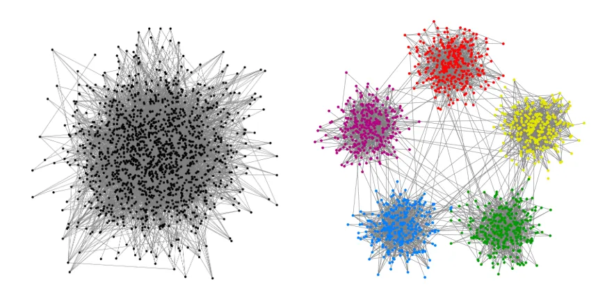
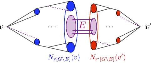
Figure 1: The above two graphs are the same graph re-organized and drawn from the SBM model with 1000 vertices, 5 balanced communities, within-cluster probability of 1/50 and across-cluster probability of 1/1000. The goal of community detection in this case is to obtain the right graph (with the true communities) from the left graph (scrambled) up to some level of accuracy. In such a context, community detection may be called graph clustering. In general, communities may not only refer to denser clusters but more generally to groups of vertices that behave similarly.
• What is a good benchmark to measure the performance of algorithms, and how good are the current algorithms?
The goal of this survey is to describe recent developments aiming at answering these ques-tions in the context of the stochastic block model. The stochastic block model (SBM) has been used widely as a canonical model for community detection. It is arguably the simplest model of a graph with communities (see definitions in the next section). Since the SBM is a generative model for the data, it benefits from a ground truth for the communities, which allows to consider the previous questions in a formal context. On the flip side, one has to hope that the model represents a good fit for real data, which does not mean necessarily a realistic model but at least an insightful one. We believe that, similarly to the role of the discrete memoryless channel in communication theory, the SBM provides such a level of insightful abstraction. The basic model captures some of the key bottleneck phenomena, and it can be extended to more advanced and realistic refinements (such edge labels or overlapping communities). Our focus will be here on the fundamental understanding of the core SBM, without diving too much into the refined extensions.
pairs of vertices with labels i and j connect independently with probability Wi,j. Further
generalizations allow for labelled edges and continuous vertex labels, connecting to low-rank approximation models and ‘graphons.’
A first hint on the centrality of the SBM comes from the fact that the model appeared independently in numerous scientific communities. It appeared under the SBM terminology in the context of social networks, in the machine learning and statistics literature Holland et al. (1983), while the model is typically called the planted partition model in theoreti-cal computer science Bui et al. (1987); Dyer and Frieze (1989); Boppana (1987), and the inhomogeneous random graph in the mathematics literature Bollob´as et al. (2007). The model takes also different interpretations, such as a planted spin-glass model Decelle et al. (2011), a sparse-graph code Abbe and Sandon (2015a,b) or a low-rank (spiked) random matrix model McSherry (2001); Vu (2014); Deshpande et al. (2015) among others.
In addition, the SBM has recently turned into more than a model for community detec-tion. It provides a fertile ground for studying various central questions in machine learning, computer science and statistics: It is rich in phase transitions Decelle et al. (2011); Mas-souli´e (2014); Mossel et al. (2014a); Abbe et al. (2016); Abbe and Sandon (2015b), allowing to study the interplay between statistical and computational barriers Y. Chen (2014); Abbe and Sandon (2015c); Banks et al. (2016); Abbe and Sandon (2017), as well as the discrepan-cies between probabilstic and adversarial models Moitra et al. (2016), and it serves as a test bed for algorithms, such as SDPs Abbe et al. (2016); B. Hajek (2014); Hajek et al. (2015c); Gu´edon and Vershynin (2016); Amini and Levina (2014); Montanari and Sen (2016); Perry and Wein (2015), spectral methods Vu (2014); Massouli´e (2014); Krzakala et al. (2013); Bordenave et al. (2015); Yun and Proutiere (2014), and belief propagation Decelle et al. (2011); Abbe and Sandon (2015).
1.2 Inference on graphs
Variants of block models where edges can have labels, or where communities can overlap, allow to cover at broad set of problems in machine learning. For example, a spiked Wigner model with observation Y =XXT +Z, whereX is an unknown vector and Z is Wigner,
can be viewed as a labeled graph where edge-(i, j)’s label is given by Yij = XiXj +Zij.
If the Xi’s take discrete values, e.g., {1,−1}, this is closely related to the stochastic block
model—see Deshpande et al. (2015) for a precise connection. The classical data clustering problem Shalev-Shwartz and Ben-David (2014), with a matrix of similarities or dissimilar-ities between n points, can also be viewed as a graph with labeled edges, and generalized block models provide probabilistic models to generate such graphs, when requiring contin-uous labels to model Euclidean connectivity kernels. In general, models where a collection of variables {Xi} have to be recovered from noisy observations {Yij} that are stochastic
functions ofXi, Xj, or more generally that depend on local interactions of some of theXi’s,
A general abstraction of these problems can also be obtained from an information the-oretic point of view, with graphical channels Abbe and Montanari (2015), themselves a special case of conditional random fields Lafferty (2001), which model conditional distribu-tions between a collection of vertex variables XV and a collection of edge variables YE on a hyper-graphG= (V, E), where the conditional probability distributions factors over each edge with a local kernelQ:
P(yE|xV) = Y
I∈E
QI(yI|x[I]),
whereyI is the realization ofY on the hyperedgeI andx[I] is the realization ofXV over the
vertices incident to the hyperedge I. Our goal in this note is to discuss tools and methods for the SBM that are likely to extend to the analysis of such general models.
1.3 Fundamental limits, phase transitions and algorithms
This note focus on thefundamental limits of community detection, with respect to various recovery requirements. The term ‘fundamental limit’ here is used to emphasize the fact that we seek conditions for recovery that are necessary and sufficient. In the information-theoretic sense, this means finding conditions under which a given task can or cannot be solved irrespective of complexity or algorithmic considerations, whereas in the computa-tional sense, this further constraints the algorithms to run in polynomial time in the num-ber of vertices. As we shall see in this note, such fundamental limits are often expressed throughphase transitionphenomena, which provide sharp transitions in the relevant regimes between phases where the given task can or cannot be resolved. In particular, identifying the bottleneck regime and location of the phase transition will typically characterize the behavior of the problem in almost any other regime.
Phase transitions have proved to be often instrumental in the developments of algo-rithms. A prominent example is Shannon’s coding theorem Shannon (1948), that gives a sharp threshold for coding algorithms at the channel capacity, and which has led the devel-opment of coding algorithms for more than 60 years (e.g., LDPC, turbo or polar codes) at both the theoretical and practical level Richardson and Urbanke (2001). Similarly, the SAT threshold Achlioptas et al. (2005) has driven the developments of a variety of satisfiability algorithms such as survey propagation M´ezard et al. (2003).
In the area of clustering and community detection, where establishing rigorous bench-marks is a long standing challenge, the quest of fundamental limits and phase transition is likely to impact the development of algorithms. In fact, this has already taken place as discussed in this note, such as with two-rounds algorithms or nonbacktracking spectral methods discussed in Section 3 and 4.
1.4 Network data analysis
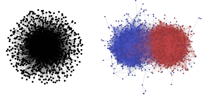
Consider the problem where one is interested in extracting features about a collection of items, in our casen= 1,222 individuals writing about US politics, observing only some form of their interactions. In our example, we have access to which blogs refers to which (via hyperlinks), but nothing else about the content of the blogs. The hope is to still extract knowledge about the individual features from these simple interactions.
To proceed, build a graph of interaction among the n individuals, connecting two in-dividuals if one refers to the other, ignoring the direction of the hyperlink for simplicity. Assume next that the data set is generated from a stochastic block model; assuming two communities is an educated guess here, but one can also estimate the number of communi-ties using the methods discussed in Section 7. The type of algorithms developed in Sections 4 and 3 can then be run on this data set, and two assortative communities are obtained. In the paper Adamic and Glance (2005), Adamic and Glance recorded which blogs are right or left leaning, so that we can check how much agreement these algorithm give with this partition of the blogs. The state-of-the-art algorithms give an agreement of roughly 95% with the groundtruth Newman (2011); Jin (2015); Gao et al. (2015). Therefore, by only observing simple pairwise interactions among these blogs, without any further information on the content of the blogs, we can infer about 95% of the blogs’ political inclinations.
Figure 2: The above graphs represent the real data set of the political blogs from Adamic and Glance (2005). Each vertex represents a blog and each edge represents the fact that one of the blogs refers to the other. The left graph is plotted with a random arrangement of the vertices, and the right graph is the output of the ABP algorithm described in Section 4, which gives 95% accuracy on the reconstruction of the political inclination of the blogs (blue and red colors correspond to left and right leaning blogs).
case, the goal is to apply such an approach to problems for which the ground truth is unknown, such as to understand biological functionality of protein complexes; to find ge-netically related sub-populations; to make accurate recommendations; medical diagnosis; image classification; segmentation; page sorting; and more.
In such cases where the ground truth is not available, a key question is to understand how reliable the algorithms’ outputs may be. On this matter, the theory discussed in this note gives a new perspective as follows. Following the definitions from Sections 4 and 3, the parameters estimated by fitting an SBM on this data set in the constant degree regime are
p1= 0.48, p2 = 0.52, Q=
52.06 5.16 5.16 47.43
. (1)
and in the logarithmic degree regime
p1= 0.48, p2= 0.52, Q=
7.31 0.73 0.73 6.66
. (2)
Following the definitions of Theorem 42 from Section 4, we can now compute the SNR for these parameters in the constant-degree regime, obtainingλ22/λ1≈18 which is much greater than 1. Thus, under an SBM model, the data is largely in a regime where communities can be detected, i.e., above the weak recovery threshold. Following the definitions of Theorem 14 from Section 3, we can also compute the CH-divergence for these parameters in the logarithmic-degree regime, obtainingJ(p, Q)≈2 which is also greater than 1. Thus, under an SBM model, the data is a regime where the graph clusters could in fact be recovered entirely, i.e, above the exact recovery threshold. This does not answer whether the SBM is a good or bad model, but it gives that under this model, the data appears in a very good ‘clustering regime.’ This is of course counting on the fact thatn= 1,222 is large enough to trust the asymptotic analysis. Had the SNR been too small, the model would have given us less confidence about the cluster outputs. This is the type of confidence insight that the study of fundamental limits can provide.
1.5 Brief historical overview of recent developments
This section provides a brief historical overview of the recent developments discussed in this monograph. The resurged interest in the SBM and its ‘modern study’ has been ini-tiated in big part due to the paper of Decelle, Krzakala, Moore, Zdeborov´a Decelle et al. (2011), which conjectured2 phase transition phenomena for the weak recovery (a.k.a. de-tection) problem at the Kesten-Stigum threshold and the information-computation gap at 4 symmetric communities in the symmetric case. These conjectures are backed in Decelle et al. (2011) with strong insights from statistical physics, based on the cavity method (belief propagation), and provide a detailed picture of the weak recovery problem, both for the
algorithmic and information-theoretic behavior. Paper Decelle et al. (2011) opened a new research avenue driven by establishing such phase transitions.
One of the first paper that obtains a non-trivial algorithmic result for the weak recovery problem is Coja-Oghlan (2010) from 2010, which appeared before the conjecture (and does not achieve the threshold by a logarithmic degree factor). The first paper to make progress on the conjecture is Mossel et al. (2015) from 2012, which proves the impossibility part of the conjecture for two symmetric communities, introducing various key concepts in the analysis of block models. In 2013, Mossel et al. (2013) also obtains a result on the partial recovery of the communities, expressing the optimal fraction of mislabelled vertices when the signal-to-noise ratio is large enough in terms of the broadcasting problem on trees Kesten and Stigum (1966); Evans et al. (2000).
The positive part of the conjecture for efficient algorithm and two communities was first proved in 2014 with Massouli´e (2014) and Mossel et al. (2014a), using respectively a spectral method from the matrix of self-avoiding walks and weighted non-backtracking walks between vertices.
In 2014, Abbe et al. (2014); Abbe et al. (2016) and Mossel et al. (2014b) found that the exact recovery problem for two symmetric communities has also a phase transition, in the logarithmic rather than constant degree regime, further shown to be efficiently achievable. This relates to a large body of work from the first decades of research on the SBM Bui et al. (1987); Dyer and Frieze (1989); Boppana (1987); Snijders and Nowicki (1997); Condon and Karp (1999); McSherry (2001); Bickel and Chen (2009); Choi et al. (2012); Vu (2014); Y. Chen (2014), driven by the exact or almost exact recovery problems without sharp thresholds.
In 2015, the phase transition for exact recovery is obtained for the general SBM Abbe and Sandon (2015b,c), and shown to be efficiently achievable irrespective of the number of communities. For the weak recovery problem, Bordenave et al. (2015) shows that the Kesten-Stigum threshold can be achieved with a spectral method based on the nonback-tracking (edge) operator in a fairly general setting (covering SBMs that are not necessarily symmetric), but falling short to settle the conjecture for more than two communities in the symmetric case due to technical reasons. The approach of Bordenave et al. (2015) is based on the ‘spectral redemption’ conjecture made in 2013 in Krzakala et al. (2013), which introduces the use of the nonbacktracking operator as a linearization of belief propagation. This is arguably the most elegant approach to the weak recovery problem, besides for the fact that the matrix is not symmetrical (to work with a symmetric matrix, the first proof of Massouli´e (2014) provides also a clean description via self-avoiding walks). The gen-eral conjecture for arbitrary many symmetric or asymmetric communities is settled later in 2015 with Abbe and Sandon (2015); Abbe and Sandon (2016b), relying on a higher-order nonbacktracking matrix and a message passing implementation. It is further shown in Abbe and Sandon (2015); Abbe and Sandon (2017) that it is possible to cross information-theoretically the Kesten-Stigum threshold in the symmetric case at 4 communities, settling both positive parts of the conjectures from Decelle et al. (2011). Crossing at 5 communities is also obtained in Banks and Moore (2016); Banks et al. (2016), which further obtains the scaling of the information-theoretic threshold for a growing number of communities.
(2015) for different distortion measures. This also gives the threshold for weak recovery in the regime where the SNR in the regime of finite SNR with diverging degrees.
Other major lines of work on the SBM have been concerned with the performance of SDPs, with a precise picture obtained in Gu´edon and Vershynin (2016); Montanari and Sen (2016); Javanmard et al. (2016) for the weak recovery problem and in Abbe et al. (2016); B. Hajek (2014); Amini and Levina (2014); Bandeira (2015); Agarwal et al. (2015); Perry and Wein (2015) for the (almost) exact recovery problem, as well as spectral methods on classical operators McSherry (2001); Coja-Oghlan (2010); Chin et al. (2015); Xu et al. (2014); Vu (2014); Yun and Proutiere (2014); Yun and Proutiere (2015). A detailed picture has also been developed for the problem of a single planted community in Montanari (2015); Hajek et al. (2015b,a); Caltagirone et al. (2016). There is a much broader list of works on the SBMs that is not covered in this paper, specially before the ‘recent developments’ discussed above but also after. It is particularly challenging to track the vast literature on this subject as it is split between different communities of statistics, machine learning, mathematics, computer science, information theory, social sciences and statistical physics. This monograph covers developments mainly until 2016. There a few additional surveys available. Community detection and more generally statistical network models are discussed in Newman (2010); Fortunato (2010); Goldenberg et al. (2010), and C. Moore has a recent overview paper Moore (2017) that focuses on the weak recovery problem with emphasis on the cavity method.
The main thresholds proved for weak and exact recovery are summarized in the table below:
Exact recovery (logarithmic degrees)
2-SSBM |√a−√b|>√2 Abbe et al. (2014); Mossel et al. (2014b) General SBM mini<jD+((P Q)i,(P Q)j)>1 Abbe and Sandon (2015b)
Weak recovery (detection) (constant degrees)
2-SSBM (a−b)2>2(a+b) Massouli´e (2014); Mossel et al. (2014a) General SBM λ2
2(P Q)> λ1(P Q) Bordenave et al. (2015); Abbe and Sandon (2015) 1.6 Outline
In the next section, we formally define the SBM and various recovery requirements for community detection, namely weak, partial and exact recovery. We then describe in Sections 3, 4, 5, 6 recent results that establish the fundamental limits for these recovery requirements. We further discuss in Section 7 the problem of learning the SBM parameters, and give a list of open problems in Section 8.
2. The Stochastic Block Model
called the planted partition model in theoretical computer science Bui et al. (1987); Dyer and Frieze (1989); Boppana (1987), and the inhomogeneous random graphs model in the mathematics literature Bollob´as et al. (2007).
2.1 The general SBM
Definition 1 Let n be a positive integer (the number of vertices), k be a positive integer (the number of communities), p = (p1, . . . , pk) be a probability vector on [k] := {1, . . . , k}
(the prior on thek communities) and W be a k×k symmetric matrix with entries in[0,1] (the connectivity probabilities). The pair(X, G)is drawn underSBM(n, p, W) ifX is ann -dimensional random vector with i.i.d. components distributed underp, andGis an n-vertex simple graph where vertices iandj are connected with probability WXi,Xj, independently of
other pairs of vertices. We also define the community sets by Ωi = Ωi(X) := {v ∈ [n] :
Xv=i}, i∈[k].
Thus the distribution of (X, G) where G = ([n], E(G)) is defined as follows, for x ∈ [k]n and y∈ {0,1}(n2),
P{X=x}:=
n Y
u=1
pxu =
k Y
i=1
p|Ωi(x)|
i (3)
P{E(G) =y|X=x}:= Y 1≤u<v≤n
Wyuv
xu,xv(1−Wxu,xv)
1−yuv (4)
= Y
1≤i≤j≤k
WNij(x,y)
i,j (1−Wi,j)N
c
ij(x,y) (5)
where,
Nij(x, y) :=
X
u<v,xu=i,xv=j
1(yuv() = 1), (6)
Nijc(x, y) := X
u<v,xu=i,xv=j
1(yuv= 0) =|Ωi(x)||Ωj(x)| −Nij(x, y), i6=j (7)
Niic(x, y) := X
u<v,xu=i,xv=i
1(yuv= 0) =|Ωi(x)|(|Ωi(x)| −1)/2−Nii(x, y), (8)
which are the number of edges and non-edges between any pair of communities. We may also talk aboutGdrawn under SBM(n, p, W) without specifying the underlying community labelsX.
Remark 2 Besides for Section 8, we assume that p does not scale with n, whereas W
typically does. As a consequence, the number of communities does not scale with n and the communities have linear size. Nonetheless, various results discussed in this note should extend (by inspection) to cases wherek is growing slowly enough.
Remark 3 Note that by the law of large numbers, almost surely,
1
Alternative definitions of the SBM require X to be drawn uniformly at random with the constraint that n1|{v∈[n] :Xv =i}|=pi+o(1), or 1n|{v∈[n] :Xv=i}|=pi for consistent
values of n and p (e.g., n/2 being an integer for two symmetric communities). For the purpose of this paper, these definitions are essentially equivalent.
2.2 The symmetric SBM
The SBM is called symmetric ifpis uniform and ifW takes the same value on the diagonal and the same value outside the diagonal.
Definition 4 (X, G) is drawn under SSBM(n, k, A, B), if p ={1/k}k and W takes value
A on the diagonal and B off the diagonal.
Note also that if all entries ofW are the same, then the SBM collapses to the Erd˝os-R´enyi random graph, and no meaningful reconstruction of the communities is possible.
2.3 Recovery requirements
The goal of community detection is to recover the labels X by observing G, up to some level of accuracy. We next define the agreement, also called sometimes overlap.
Definition 5 (Agreement) The agreement between two community vectors x, y∈[k]n is obtained by maximizing the common components between x and any relabelling ofy, i.e.,
A(x, y) = max
π∈Sk
1
n
n X
i=1
1(xi=π(yi)), (9)
where Sk is the group of permutations on [k].
Note that the relabelling permutation is used to handle symmetric communities such as in SSBM, as it is impossible to recover the actual labels in this case, but we may still hope to recover the partition. In fact, one can alternatively work with the community partition Ω = Ω(X), defined earlier as the unordered collection of the k disjoint unordered subsets Ω1, . . . ,Ωkcovering [n] with Ωi ={u∈[n] :Xu=i}. It is however often convenient to work
with vertex labels. Further, upon solving the problem of finding the partition, the problem of assigning the labels is often a much simpler task. It cannot be resolved if symmetry makes the community label non identifiable, such as for SSBM, and it is trivial otherwise by using the community sizes and clusters/cuts densities.
For (X, G) ∼ SBM(n, p, W) one can always attempt to reconstruct X without even taking into account G, simply drawing each component of ˆX i.i.d. under p. Then the agreement satisfies almost surely
A(X,Xˆ)→ kpk22, (10)
andkpk2
2= 1/kin the case ofpuniform. Thus an agreement becomes interesting only when it is above this value.
One can alternatively define a notion of component-wise agreement. Define the overlap between two random variablesX, Y on [k] as
O(X, Y) = X
z∈[k]
and O∗(X, Y) = maxπ∈SkO(X, π(Y)). In this case, for X,Xˆ i.i.d. under p, we have O∗(X,Xˆ) = 0.
All recovery requirement in this note are going to be asymptotic, taking place with high probability as n tends to infinity. We also assume in the following sections—except for Section 7—that the parameters of the SBM are known when designing the algorithms.
Definition 6 Let (X, G) ∼SBM(n, p, W). The following recovery requirements are solved if there exists an algorithm that takes G as an input and outputsXˆ = ˆX(G) such that
• Exact recovery: P{A(X,Xˆ) = 1}= 1−o(1),
• Almost exact recovery: P{A(X,Xˆ) = 1−o(1)}= 1−o(1),
• Partial recovery: P{A(X,Xˆ)≥α}= 1−o(1), α∈(0,1).
In other words, exact recovery requires the entire partition to be correctly recovered, almost exact recovery allows for a vanishing fraction of misclassified vertices and partial recovery allows for a constant fraction of misclassified vertices. We callαthe agreement or accuracy of the algorithm.
Different terminologies are sometimes used in the literature, with following equivalences:
• exact recovery ⇐⇒ strong consistency
• almost exact recovery ⇐⇒ weak consistency
Sometimes ‘exact recovery’ is also called just ‘recovery’ and ‘almost exact recovery’ is called ‘strong recovery.’
As mentioned above, that values of α that are too small may not be interesting or possible. In the symmetric SBM with k communities, an algorithm that that ignores the graph and simply draws ˆX i.i.d. under p achieves an accuracy of 1/k. Thus the problem becomes interesting whenα >1/k, leading to the following definition.
Definition 7 Weak recovery or detection is solved in SSBM(n, k, A, B) if for (X, G) ∼
SSBM(n, k, A, B), there existsε >0and an algorithm that takes Gas an input and outputs ˆ
X such thatP{A(X,Xˆ)≥1/k+ε}= 1−o(1).
Equivalently, P{O∗(XV,XˆV) ≥ε} = 1−o(1) where V is uniformly drawn in [n].
De-termining the counterpart of weak recovery in the general SBM requires some discussion. Consider an SBM with two communities of relative sizes (0.8,0.2). A random guess un-der this prior gives an agreement of 0.82+ 0.22 = 0.68, however an algorithm that simply puts every vertex in the first community achieves an agreement of 0.8. In Decelle et al. (2011), the latter agreement is considered as the one to improve upon in order to detect communities, leading to the following definition:
As shown in Abbe and Sandon (2017), previous definition is however not the right definition to capture the Kesten-Stigum threshold in the general case. In other words, the conjecture that max-detection is always possible above the Kesten-Stigum threshold is not accurate in general SBMs. Back to our example with communities of relative sizes (0.8,0.2), an algorithm that could find a set containing 2/3 of the vertices from the large community and 1/3 of the vertices from the small community would not satisfy the above above detection criteria, while the algorithm produces nontrivial amounts of evidence on what communities the vertices are in. To be more specific, consider a two community SBM where each vertex is in community 1 with probability 0.99, each pair of vertices in community 1 have an edge between them with probability 2/n, while vertices in community 2 never have edges. Regardless of what edges a vertex has it is more likely to be in community 1 than community 2, so detection according to the above definition is not impossible, but one can still divide the vertices into those with degree 0 and those with positive degree to obtain a non-trivial detection—see Abbe and Sandon (2017) for a formal counter-example.
A fix fo this issue is to consider a weighted notion of agreement, i.e.,
˜
A(x, y) = max
π∈Sk
1
k
k X
i=1
P
u∈[n]1(xu=π(yu), xu =i) P
u∈[n]1(xu =i)
, (12)
which counts the number of agreeing components (up to relabellings) normalized by the size of the communities. Weak recovery (or detection) can then be defined as obtaining with high probability a weighted agreement of
˜
A(X,Xˆ(G)) = 1/k+ Ωn(1),
and this applies to the general SBM. Another definition of detection that seems easier to manipulate and that implies the previous one is as follows; note that this definition requires a single partition even for the general SBM.
Definition 9 Weak recovery or detection is solved in SBM(n, p, W) if for (X, G) ∼
SBM(n, p, W), there exists ε >0, i, j ∈[k] and an algorithm that takes Gas an input and outputs a partition of [n]into two sets (S, Sc) such that
P{|Ωi∩S|/|Ωi| − |Ωj∩S|/|Ωj| ≥}= 1−o(1),
where we recall that Ωi={u∈[n] :Xu =i}.
In other words, an algorithm solves detection if it divides the graph’s vertices into two sets such that vertices from two different communities have different probabilities of being assigned to one of the sets. With this definition, putting all vertices in one community does not detect, since |Ωi ∩S|/|Ωi| = 1 for all i ∈ [k]. Further, in the symmetric SBM, this
definition implies Definition 7 provided that we fix the output:
See Abbe and Sandon (2016b) for the proof. The above is likely to extend to other weakly symmetric SBMs, i.e., that have constant expected degree, but not all.
Finally, note that our notion of detection requires to separate at least two communities
i, j∈[k]. One may ask for a definition where two specific communities need to be separated:
Definition 11 Separation of communitiesiandj, withi, j∈[k], is solved inSBM(n, p, W) if for(X, G)∼SBM(n, p, W), there existsε >0and an algorithm that takes G as an input and outputs a partition of [n] into two sets(S, Sc) such that
P{|Ωi∩S|/|Ωi| − |Ωj∩S|/|Ωj| ≥}= 1−o(1).
There are at least two additional questions that are natural to ask about SBMs, both can be asked for efficient or information-theoretic algorithms:
• Distinguishability or testing: Consider an hypothesis test where a random graph
Gis drawn with probability 1/2 from an SBM model (with same expected degree in each community) and with probability 1/2 from an Erd˝os-R´enyi model with matching expected degree. Is is possible to decide with asymptotic probability 1/2 +εfor some
ε > 0 from which ensemble the graph is drawn? This requires the total variation between the two ensembles to be non-vanishing. This is also sometimes called ‘detec-tion’, although we use here detection as an alternative terminology to weak recovery. Distinguishability is further discussed in Section 4.6.1.
• Learnability: Assume that G is drawn from an SBM ensemble, is it possible to obtain a consistent estimator for the parameters? E.g., can we learn k, p, Q from a graph drawn from SBM(n, p, Q/n)? This is further discussed in Section 7.
The obvious implications are: exact recovery ⇒ almost exact recovery ⇒ partial recovery
⇒weak detection⇒distinguishability. Moreover, for symmetric SBMs with two symmetric communities: learnability ⇔ weak recovery ⇔ distinguishability, but these are broken for general SBMs; see Section 7.
2.4 Model variants
There are various extensions of the basic SBM discussed in previous section, in particular:
• Labelled SBMs: allowing for edges to carry a label, which can model intensities of similarity functions between vertices (see for example Heimlicher et al. (2012); Xu et al. (2014); Jog and Loh (2015); Yun and Proutiere (2015) and further details in Section 3.5);
• Degree-corrected SBMs: allowing for a degree parameter for each vertex that scales the edge probabilities in order to makes expected degrees match the observed degrees (see for example Karrer and Newman (2011);?);?);
Another variant that circumvents the discussions about non-edges is to consider acensored block model(CBM), defined as follows (see Abbe et al. (2014a)).
Definition 12 (Binary symmetric CBM) Let G = ([n], E) be a graph and ε ∈ [0,1]. Let Xn= (X1, . . . , Xn) with i.i.d. Bernoulli(1/2)components. Let Y be a random vector of
dimension n2 taking values in {0,1, ?} such that
P{Yij = 1|Xi =Xj, Eij = 1}=P{Yij = 0|Xi 6=Xj, Eij = 1}=ε (13)
P{Yij =?|Eij = 0}= 1. (14)
The case of an Erdos-Renyi graph is discussed in Heimlicher et al. (2012); Abbe et al. (2014a,b); Chin et al. (2015); Saade et al. (2015); Chen et al. (2014); Chen and Goldsmith (2014). Inserting the ? symbol simplifies a few aspects compared to SBMs with respect to non-edges. In that sense, the CBM is a more convenient model than the SBM from a mathematical viewpoint, while behaving similarly to the SBM (when G is an Erdos-Renyi graph of degree (a+b)/2 and ε=b/(a+b) for the two community symmetric case). The CBM can also be viewed as a synchronization model over the binary field, and more general synchronization models have been studied in ??, with a complete description both at the fundamental and algorithmic level (generalizing in particular the results from Section 6.2). Further, one can consider more general models of inhomogenous random graphs Bollob´as et al. (2007), which attach to each vertex a label in a set that is not necessar-ily finite, and where edges are drawn independently from a given kernel conditionally on these labels. This gives in fact a way to model mixed-membership, and is also related to graphons, which corresponds to the case where each vertex has a continuous label.
It may be worth saying a few words about the theory of graphons and its implications for us. Lov´asz and co-authors introduced graphons Lov´asz and Szegedy (2006); Borgs et al. (2008); Lov´asz (2012) in the study of large graphs (also related to Szemer´edi’s Regular-ity Lemma Szemer´edi (1976)), showing that3 a convergent sequence of graphs admits a limit object, the graphon, that preserves many local and global properties of the sequence. Graphons can be represented by a measurable function w : [0,1]2 → [0,1], which can be viewed as a continuous extensions of the connectivity matrix W used throughout this pa-per. Most relevant to us is that any network model that is invariant under node labelings, such as most models of practical interests, can be described by an edge distribution that is conditionally independenton hidden node labels, via such a measurable mapw. This gives a de Finetti’s theorem for label-invariant models Hoover (1979); Aldous (1981); Diaconis and Janson (2007), but does not require the topological theory behind it. Thus the theory of graphons may give a broader meaning to the study of block models, which are precisely building blocks to graphons, but for the sole purpose of studying exchangeable network models, inhomogeneous random graphs give enough degrees of freedom.
Further, many problems in machine learning and networks are also concerned with interactions of items that go beyond the pairwise setting. For example, citation or metabolic networks rely on interactions amongk-tuples of vertices. In a broad context, one may thus cast the SBM and its variants into a a comprehensive class of conditional random field or
channel model, where edges labels depend on vertex labels,4 such as developed in Abbe and Montanari (2015) withgraphical channels as follows.
LetV = [n] andG= (V, E(G)) be a hypergraph withN =|E(G)|. LetX andY be two finite sets called respectively the input and output alphabets, andQ(·|·) be a channel from
Xk toY called the kernel. To each vertex in V, assign a vertex-variable inX, and to each
edge in E(G), assign an edge-variable in Y. Let yI denote the edge-variable attached to
edge I, and x[I] denote the k node-variables adjacent toI. We define a graphical channel with graph Gand kernelQas the channel P(·|·) given by
As we shall see for the SBM, two quantities are key to understand how much information can be carried in graphical channels: a measure on how “rich” the observation graphGis, and a measure on how “noisy” the connectivity kernel Q is. This survey quantifies the tradeoffs between these two quantities in the SBM (which corresponds to a discrete X, a complete graph G and a specific kernel Q), in order to recover the input from the output. Similar tradeoffs are expected to take place in other graphical channels, such as in ranking, synchronization, topic modelling or other related models.
2.5 SBM regimes and topology
Before discussing when the various recovery requirements can be solved or not in SBMs, it is important to recall a few topological properties of the SBM graph.
When all the entries ofW are the same and equal tow, the SBM collapses to the Erd˝ os-R´enyi model G(n, w) where each edge is drawn independently with probability w. Let us recall a few basic results for this model derived mainly from Erd¨os and R´enyi (1960):
• G(n, cln(n)/n) is connected with high probability if and only if c >1,
• G(n, c/n) has a giant component (i.e., a component of size linear in n) if and only if
c >1,
• For δ < 1/2, the neighborhood at depth r =δlogcn of a vertex v in G(n, c/n), i.e.,
B(v, r) = {u ∈ [n] : d(u, v) ≤ r} where d(u, v) is the length of the shortest path connectingu andv, tends in total variation to a Galton-Watson branching process of offspring distribution Poisson(c).
For SSBM(n, k, A, B), these results hold by essentially replacing c with the average degree.
• Fora, b >0, SSBM(n, k, alogn/n, blogn/n) is connected with high probability if and only if a+(kk−1)b >1 (ifaorb is equal to 0, the graph is of course not connected). 4. A recent paper Berthet et al. (2016) has also considered an Ising model with block structure, studying
• SSBM(n, k, a/n, b/n) has a giant component (i.e., a component of size linear in n) if and only if d:= a+(kk−1)b >1,
• Forδ <1/2, the neighborhood at depthr =δlogdnof a vertexvin SSBM(n, k, a/n, b/n) tends in total variation to a Galton-Watson branching process of offspring distribution Poisson(d) where dis as above.
Similar results hold for the general SBM, at least for the case of a constant excepted degrees. For connectivity, one has that SBM(n, p, Qlogn/n) is connected with high proba-bility if
min
i∈[k]
k(diag(p)Q)ik1>1 (15)
and is not connected with high probability if mini∈[k]k(diag(p)Q)ik1<1, where (diag(p)Q)i
is the i-th column of diag(p)Q.
These results are important to us as they already point regimes where exact or weak recovery is not possible. Namely, if the SBM graph is not connected, exact recovery is not possible (since there is no hope to label disconnected components with higher chance than 1/2), hence exact recovery can take place only if the SBM parameters are in the logarithmic degree regime. In other words, exact recovery in SSBM(n, k, alogn/n, blogn/n) is not solvable if a+(kk−1)b < 1. This is however unlikely to provide a tight condition, i.e., exact recovery is not equivalent to connectivity, and next section will precisely investigate how much more than a+(kk−1)b >1 is needed to obtain exact recovery. Similarly, it is not hard to see that weak recovery is not solvable if the graph does not have a giant component, i.e., weak recovery is not solvable in SSBM(n, k, a/n, b/n) if a+(kk−1)b < 1, and we will see in Section 4 how much more is needed to go from the giant to weak recovery.
2.6 Challenges: spectral, SDP and message passing approaches
Consider the symmetric SBM with two communities, where the inner-cluster probability is
a/nand the across-cluster probability isb/n, i.e., SSBM(n,2, a/n, b/n), and assume a≥b. We next discuss basic approaches and the challenges that they face.
The spectral approach. Assume for simplicity that the two clusters have exactly size
n/2, and index the first cluster with the first n/2 vertices. The expected adjacency matrix EA of this graph has four blocks given by
EA=
a/n·1n/2×n/2 b/n·1n/2×n/2
b/n·1n/2×n/2 a/n·1n/2×n/2
. (16)
This matrix has three eigenvalues, namely (a+b)/n, (a−b)/nand 0, where 0 has multiplicity
n−2, and eigenvectors attached to the first two eigenvalues are
a+b n ,
1n/2 1n/2
,
a−b n ,
1n/2
−1n/2
. (17)
eigenvector corresponding to the second largest eigenvalue, and assigning each vertex to a community depending on the sign of this eigenvector’s components. Of course, we do not have access to the expected adjacency matrix, nor a tight estimate since we are observing a single shot of the SBM graph, but we can view the adjacency matrixAas a perturbation of EA, i.e.,
A=EA+Z
whereZ = (A−EA) is the perturbation. One may hope that this perturbation is moderate, i.e., that carrying the same program as for the expected adjacency—taking the second eigenvector of A—still gives a meaningful reconstruction of the communities.
The Courant-Fisher theorem can be used to obtain a simple control on the perturbation of the eigenvalues of A from EA. Denoting by λ1 ≥ · · · ≥λn and ˆλ1 ≥ˆλ2 ≥ · · · ≥λˆn the
ordered eigenvalues ofEA and A respectively, we have for alli∈[n],
|λi−λˆi| ≤ kZk, (18)
where k · k denotes the operator norm. Thus, if kZk is less than half of the least gap between the three eigenvalues a+nb, a−nb and 0, the eigenvalues ofA would have a preserved ordering. This would only give us hope that the eigenvectors would be correlated, but gives no guarantees so far. The Davis-Kahan Theorem can be used to that end, giving that the angleθibetween the eigenvectors corresponding to thei-th eigenvalues has a sinus bounded
as sinθi ≤ min kZk
i6=j|λi−λj|/2 (this is in fact a slightly weaker statement than Davis-Kahan).
Thus estimating the operator norm is crucial with this approach, and tools from random matrix theory can be used here Nadakuditi and Newman (2012); Vu (2007).
The problem with this naive approach is that it fails when a and bare too small, such as in the sparse regime (constant a, b) or even slowly growing degrees. One of the main reasons for this is that the eigenvalues are far from being properly ordered in such cases, in particular due to high degree nodes. In the sparse regime, there will be nodes of almost logarithmic degree, and these induce eigenvalues of order roughly root-logarithmic. To see this, note that an isolated star graph, i.e., a single vertex connected to k neighbors, has an eigenvalue of √k with eigenvector having weight 1 on the center-vertex and √k on the neighbors (recall that applying a vector to the adjacency matrix corresponds to diffusing each vector component to its neighbors).
The message passing approach. Before describing the approach, let us remind ourselves of what our goals are. We defined different recovery requirements for the SBM, in particular weak and exact recovery. As discussed in Section 3, exact recovery yields a clear target for the SSBM, the optimal algorithm (minimizing the probability of failing) is the Maximum A Posteriori (MAP) algorithm that looks for the min-bisection:
ˆ
xmap(g) = arg max
x∈{+1,−1}n xt1n=0
xtAx, (19)
which is equivalent to finding a balanced±1 assignment to each vertex such that the number of edges with different end points is minimized. This is NP-hard in the worst-case (due to the integral constraint), but we will show that the min-bisection can be found efficiently ‘with high probability’ for the SBM whenever it is unique with high probability (i.e., no gap occurs!). Further, both the spectral approach described above (with some modifications) and the SDP approach described in Section 3.4 allow to achieve the threshold, and each can be viewed as a relaxation of the min-bisection problem (see Section 3.4).
For weak recovery instead, minimizing the error probability (i.e., the MAP estimator) is no longer optimal, and thus targeting the min-bisection is not necessarily the right approach. As discussed above, the spectral approach on the adjacency matrix can fail dramatically, as it will catch localized eigenvectors (e.g., high-degree nodes) rather than communities. The SDP approach seems more robust. While it does not detect communities in the most challenging regimes, it approaches the threshold fairly closely for two communities—see Javanmard et al. (2016). Nonetheless, it does not target the right figure of merit for weak recovery.
What is then the right figure of merit for weak recovery? Consider the agreement metric, i.e., minimizing the fraction of mislabelled vertices. Consider also a perturbation of the SBM parameters to a slightly asymmetric version, such that the labels can now be identified from the partition, to avoid the relabelling maximization over the communities. The agreement between the true clustersXand a reconstruction ˆXis then given byP
v∈[n]1(Xv = ˆXv(G)),
and upon observingG=g, the expected agreement is maximized by finding for eachv∈[n]
max ˆ
xv
P{Xv= ˆxv|G=g}. (20)
The reasons for considering an asymmetric SBM here is that the above expression is exactly equal to half in the symmetric case, which carries no information. To remediate to that, one should break the symmetry in the symmetric case by revealing some vertex labels (or use noisy labels as done in Deshpande et al. (2015), or parity of pairs of vertices). One may also relate the random agreement to its expectation with concentration arguments. These are overlooked here, but we get a hint on what the Bayes optimal algorithm should do: it should approximately maximize the posterior distribution of a single vertex given the graph. This is different than MAP which attempts to recover all vertices in one shot. In the latter context, the maximizer may not be ‘typical’ (e.g., the all-one vector is the most likely outcome of n i.i.d. Bernoulli(3/4) random variables, but it does not have a typical fraction of 1’s).
a tight approximation. When the graph is a tree, the approximation is exact, and physicists have good reasons to believe that this remains true even in our context of a loopy graph Decelle et al. (2011). However, establishing such a claim rigorously is a long-standing challenge for message passing algorithms. Without a good guess on how to initialize BP, which we do not possess for the detection problem, one may simply take a random initial guess. In the symmetric case, this would still give a bias of roughly√n vertices (from the Central Limit Theorem) towards the true partition, i.e., a initial belief of 1/2 + Θ(1/√n) towards the truth. Recall that in BP, each vertex will send its belief of being 0 or 1 to its neighbors, computing this belief using Bayes rule from the received beliefs at previous iteration, and factoring out the backtracking beliefs (i.e., do not take into account the belief of a specific vertex to update it in the next iteration). As the initial belief of 1/2 is a trivial fix point in BP, one may attempt to approximate the update Bayes rule around the uniform beliefs, working out the linear approximation of the BP update. This gives raise to a linear operator, which is the nonbacktracking (NB) operator discussed in Section 4.5.1, and running linerazied BP corresponds to taking a power-iteration method with this operator on the original random guesses—see Section 4.5.1. Thus, we are back to a spectral method, but with an operator that is a linearization of the Bayes optimal approximation (this gave raise to the terminology ‘spectral redemption’ in Krzakala et al. (2013).)
The advantage of this linearized approach is that it is easier to analyze than the full BP, and one can prove statements about it, such as that it detects down to the optimal threshold Bordenave et al. (2015); Abbe and Sandon (2015). On the other hand, linerarized BP will loose some accuracy in contrast to full BP, but this can be improved by using a two-round algorithm: start with linearized BP to provably detect communities, and then enhance this reconstruction by feeding it to full BP—see for example Mossel et al. (2013); Abbe and Sandon (2016b). The latter approach gives raise to a new approach to analyzing belief propagation: can such two rounds approaches with linearization plus amplification be applied to other problems?
3. Exact Recovery
3.1 Fundamental limit and the CH threshold
Exact recovery for linear size communities has been one of the most studied problem for block models in its first decades. A partial list of papers is given by Bui et al. (1987); Dyer and Frieze (1989); Boppana (1987); Snijders and Nowicki (1997); Condon and Karp (1999); McSherry (2001); Bickel and Chen (2009); Choi et al. (2012); Vu (2014); Y. Chen (2014). In this line of work, the approach is mainly driven by the choice of the algorithms, and in particular for the model with two symmetric communities. The results look as follows5:
Bui, Chaudhuri,
Leighton, Sipser ’84 maxflow-mincut A= Ω(1/n), B=o(n−1−4/((A+B)n)) Boppana ’87 spectral meth. (A−B)/√A+B = Ω(plog(n)/n) Dyer, Frieze ’89 min-cut via degrees A−B= Ω(1)
Snijders, Nowicki ’97 EM algo. A−B= Ω(1)
Jerrum, Sorkin ’98 Metropolis aglo. A−B= Ω(n−1/6+) Condon, Karp ’99 augmentation algo. A−B= Ω(n−1/2+) Carson, Impagliazzo ’01 hill-climbing algo. A−B = Ω(n−1/2log4(n)) McSherry ’01 spectral meth. (A−B)/√A≥Ω(plog(n)/n) Bickel, Chen ’09 N-G modularity (A−B)/√A+B= Ω(log(n)/√n) Rohe, Chatterjee, Yu ’11 spectral meth. A−B= Ω(1)
More recently, Vu Vu (2014) obtained a spectral algorithm that works in the regime where the expected degrees are logarithmic, rather than poly-logarithmic as in McSherry (2001); Choi et al. (2012). Note that exact recovery requires the node degrees to be at least logarithmic, as discussed in Section 2.5. Thus the results of Vu are tight in the scaling, and the first to apply in such great generality, but as for the other results in Table 1, they do not reveal the phase transition. The fundamental limit for exact recovery was derived first for the case of symmetric SBMs with two communities:
Theorem 13 Abbe et al. (2014); Mossel et al. (2014b) Exact recovery inSSBM(n,2, aln(n)/n, bln(n)/n) is solvable and efficiently so if |√a−√b|>√2 and unsolvable if|√a−√b|<√2.
A few remarks regarding this result:
• At the threshold, one has to distinguish two cases: ifa, b >0, then exact recovery is solvable (and efficiently so) if|√a−√b|=√2 as first shown in Mossel et al. (2014b). If aor b are equal to 0, exact recovery is solvable (and efficiently so) if √a > √2 or
√
b >√2 respectively, and this corresponds to connectivity.
• Theorem 13 provides a necessary and sufficient condition for exact recovery, and covers all cases for exact recovery in SSBM(n,2, A, B) were A and B may depend on n as long as not asymptotically equivalent (i.e., A/B 9 1). For example, if A = 1/
√
n
and B = ln3(n)/n, which can be written as A =
√
n
lnn
lnn
n and B = ln
2nlnn n , then
exact recovery is trivially solvable as |√a−√b|goes to infinity. If insteadA/B→1, then one needs to look at the second order terms. This is covered by Mossel et al. (2014b) for the 2 symmetric community case, which shows that for an, bn = Θ(1),
exact recovery is solvable if and only if ((√an− √
bn)2−1) logn+ log logn/2 =ω(1). • Note that |√a −√b| > √2 can be rewritten as a+2b > 1 + √ab and recall that
a+b
2 >2 is the connectivity requirement in SSBM. As expected, exact recovery requires connectivity, but connectivity is not sufficient. The extra term √ab is the ‘over-sampling’ factor needed to go from connectivity to exact recovery, and the connectivity threshold can be recovered by considering the case where b = 0. An information-theoretic interpretation of Theorem 13 is also discussed below.
Theorem 14 Abbe and Sandon (2015b) Exact recovery inSBM(n, p,ln(n)Q/n) is solvable and efficiently so if
I+(p, Q) := min
1≤i<j≤kD+((diag(p)Q)ik(diag(p)Q)j)>1
and is not solvable if I+(p, Q)<1, where D+ is defined by
D+(µkν) := max
t∈[0,1]
X
x
ν(x)ft(µ(x)/ν(x)), ft(y) := 1−t+ty−yt. (21)
Remark 15 Regarding the behavior at the threshold: If all the entries ofQ are non-zero, then exact recovery is solvable (and efficiently so) if and only if I+(p, Q) ≥1. In general, exact recovery is solvable at the threshold, i.e., when I+(p, Q) = 1, if and only if any two columns ofdiag(p)Qhave a component that is non-zero and different in both columns.
Remark 16 In the symmetric caseSSBM(n, k, aln(n)/n, bln(n)/n), the CH-divergence is maximized at the value of t = 1/2, and it reduces in this case to the Hellinger divergence between any two columns of Q; the theorem’s inequality becomes
1
k(
√
a−√b)2 >1,
matching the expression obtained in Theorem 13 for 2 symmetric communities.
We discuss now some properties of the functional D+ governing the fundamental limit for exact recovery in Theorem 14. For t∈[0,1], let
Dt(µkν) := X
x
ν(x)ft(µ(x)/ν(x)), ft(y) = 1−t+ty−yt, (22)
and note that D+= maxt∈[0,1]Dt. Since the function ftsatisfies • ft(1) = 0
• ft is convex on R+,
the functional Dt is what is called an f-divergence Csisz´ar (1963), like the KL-divergence
(f(y) =ylogy), the Hellinger divergence, or the Chernoff divergence. Such functionals have a list of common properties described in Csisz´ar (1963). For example, if two distributions are perturbed by additive noise (i.e., convolving with a distribution), then the divergence al-ways increases, or if some of the elements of the distributions’ support are merged, then the divergence always decreases. Each of these properties can interpreted in terms of commu-nity detection (e.g., it is easier to recovery merged communities, etc.). Since Dt collapses
to the Hellinger divergence when t = 1/2 and since it matches the Chernoff divergence for probability measures, we call Dt the Chernoff-Hellinger (CH) divergence in Abbe and
Sandon (2015b), and so for D+ as well by a slight abuse of terminology.
3.2 Proof techniques
Let (X, G) ∼ SBM(n, p, W). Recall that to solve exact recovery, we need to find the partition of the vertices, but not necessarily the actual labels. Equivalently, the goal is to find the community partition Ω = Ω(X) as defined in Section 2. Upon observing G= g, reconstructing Ω with ˆΩ(g) gives a probability of error given by
Pe:=P{Ω6= ˆΩ(G)}= X
g
P{Ω(ˆ g)6= Ω|G=g}P{G=g} (23)
and thus an estimator ˆΩmap(·) minimizing the above must minimize P{Ω(ˆ g) 6= Ω|G =g} for every g. To minimizeP{Ω(ˆ g) 6= Ω|G=g}, we must declare a reconstruction ofs that maximizes the posterior distribution
P{Ω =s|G=g}, (24)
or equivalently
X
x∈[k]n:Ω(x)=s
P{G=g|X=x} k Y
i=1
p|Ωi(x)|
i , (25)
and any such maximizer can be chosen arbitrarily.
This defines the MAP estimator ˆΩmap(·), which minimizes the probability of making an error for exact recovery. If MAP fails in solving exact recovery, no other algorithm can succeed. Note that to succeed for exact recovery, the partition shall be typical in order to make the last factor in (25) non-vanishing (i.e., communities of relative size pi +o(1)
for all i ∈ [k]). Of course, resolving exactly the maximization in (24) requires comparing exponentially many terms, so the MAP estimator may not always reveal the computational threshold for exact recovery.
3.2.1 Converse: the genie-aided approach
We now describe how to obtain the impossibility part of Theorem 14. Imagine that in addition to observing G, a genie provides the observation of X∼u ={Xv :v ∈[n]\ {u}}.
Define now ˆXv =Xv forv∈[n]\ {u} and
ˆ
Xu,map(g, x∼u) = arg max i∈[k]P
{Xu =i|G=g, X∼u =x∼u}, (26)
where ties can be broken arbitrarily if they occur (we assume that an error is declared in case of ties to simplify the analysis). If we fail at recovering a single component when all others are revealed, we must fail at solving exact recovery all at once, thus
P{Ωmap(ˆ G)6= Ω} ≥P{∃u∈[n] : ˆXu,map(G, X∼u)6=Xu}. (27)
considered. In any case, studying when this lower bound is not vanishing always provides a necessary condition for exact recovery.
Let Eu :={Xˆu,map(G, X∼u)6=Xu}. If the eventsEu were independent, we could write
P{∪uEu}= 1−P{∩uEuc}= 1−(1−P{E1})n≥1−e−nP{E1} and if P{E1}=ω(1/n), this would drive P{∪uEu}, and thus Pe, to 1. The events Eu are not independent, but their
dependencies are weak enough such that previous reasoning still applies, and Pe is driven
to 1 whenP{E1}=ω(1/n).
Formally, one can handle the dependencies with different approaches. We describe here an approach via the second moment method. Recall the following basic inequality.
Lemma 17 If Z is a random variable taking values in Z+={0,1,2, . . .}, then P{Z = 0} ≤ VarZ
(EZ)2. We apply this inequality to
Z= X
u∈[n]
1( ˆXu,map(G, X∼u)6=Xu),
which counts the number of components where component-MAP fails. Note that the right hand side of (27) corresponds toP{Z≥1}as desired. Our goal is to show that (VEarZZ)2 stays
strictly below 1 in the limit, or equivalently, (EEZZ2)2 stays strictly below 2 in the limit. In
fact, the latter tends to 1 in the converse of Theorem 14. Note that Z = P
u∈[n]Zu where Zu := 1( ˆXu,map(G, X∼u) 6= Xu) are binary random
variables withEZu =EZv for all u, v. Hence,6
EZ =nP{Z1 = 1} (28)
EZ2 = X
u,v∈[n]
E(ZuZv) = X
u,v∈[n]
P{Zu =Zv= 1} (29)
=nP{Z1 = 1}+n(n−1)P{Z1= 1}P{Z2= 1|Z1= 1} (30) and (EEZZ2)2 tends to 1 if
nP{Z1 = 1}+n(n−1)P{Z1= 1}P{Z2= 1|Z1= 1}
n2P{Z
1= 1}2
= 1 +o(1) (31)
or
1
nP{Z1= 1}
+ P{Z2 = 1|Z1 = 1} P{Z1= 1}
= 1 +o(1). (32)
This takes place ifnP{Z1= 1}diverges and P{Z2 = 1|Z1 = 1}
P{Z2= 1}
= 1 +o(1), (33)
i.e., if E1, E2 are asymptotically independent.
The asymptotic independence takes place due to the regime that we consider for the block model in the theorem. To given a related example, in the context of the Erd˝os-R´enyi modelER(n, p), ifW1 is 1 when vertexuis isolated and 0 otherwise, thenP{W1= 1|W2= 1}= (1−p)n−2 andP{W1= 1}= (1−p)n−1, and thus P{WP{1=1W|W2=1}
1=1} = (1−p)
−1 tends to 1 as long as p tends to 0. That is, the property of a vetex being isolated is asymptotically independent as long as the edge probability is vanishing. A similar outcomes takes place for the property of MAP-component failing when edge probabilities are vanishing in the block model.
The location of the threshold is then dictated by requirement thatnP{Z1 = 1}diverges, and this where the CH-divergence threshold emerges from a moderate deviation analysis. We next summarize what we obtained with the above reasoning, and then specialized to the regime of Theorem 14.
Theorem 18 Let (X, G)∼SBM(n, p, W) and Zu :=1( ˆXu,map(G, X∼u)6=Xu), u∈[n]. If
p, W are such that E1 and E2 are asymptotically independent, then exact recovery is not solvable if
P{Xˆu,map(G, X∼u)=6 Xu}=ω(1/n). (34)
The next lemma gives the behavior of P{Z1= 1}in the logarithmic degree regime.
Lemma 19 Abbe and Sandon (2015b) Consider the hypothesis test where H=ihas prior probabilitypi fori∈[k], and where observableY is distributedBin(np, Wi)under hypothesis
H = i. Then the probability of error Pe(p, W) of MAP decoding for this test satisfies
1
k−1Over(n, p, W)≤Pe(p, W)≤Over(n, p, W) where Over(n, p, W) =X
i<j X
z∈Zk
+
min(P{Bin(np, Wi) =z}pi,P{Bin(np, Wj) =z}pj),
and for a symmetric Q∈Rk+×k,
Over(n, p,log(n)Q/n) =n−I+(p,Q)−O(log log(n)/logn), (35)
where I+(p, Q) = mini<jD+((diag(p)Q)i,(diag(p)Q)j).
Corollary 20 Let (X, G)∼SBM(n, p, W) where p is constant and W =Qlnnn. Then P{Xˆu,map(G, X∼u)6=Xu}=n−I+(p,Q)+o(1). (36)
A robust extension of this Lemma is proved in Abbe and Sandon (2015b) that allows for a slight perturbation of the binomial distributions. We next explain why E1 and E2 are asymptotically independent.
Recall that Z1 =1( ˆX1,map(G, X∼1) 6=X1), and E1 is the event thatZ1 = 1, i.e., that
Gand X take values gand x such that7
argmaxi∈[k]P{X1 =i|G=g, X∼1=x∼1} 6=x1. (37) 7. Formally, argmax is a set, and we are asking that this set is not the singleton{x1}. It could be that this
set is not that singleton but contains x1, in which case breaking ties may still make component-MAP
Letx∼1∈[k]n−1 and ω(x∼1) :i=|Ωi(x∼1)|. We have
P{X1 =x1|G=g, X∼1=x∼1} (38)
∝P{G=g|X∼1 =x∼1, X1 =x1} ·P{X∼1=x∼1, X1=x1} (39)
∝P{G=g|X∼1 =x∼1, X1 =x1}P{X1 =x1} (40)
=p(x1)
Y
1≤i<j≤k
WNij(x∼1,g)
i,j (1−Wi,j)N
c
ij(x∼1,g) (41)
· Y
1≤i≤k
WN
(1)
i (x∼1,g)
i,x1 (1−Wi,x1)
ωi(x∼1)−Ni(1)(x∼1,g) (42)
∝p(x1)
Y
1≤i≤k
WN
(1)
i (x∼1,g)
i,x1 (1−Wi,x1)
ωi(x∼1)−Ni(1)(x∼1,g) (43)
whereNi(1)(x∼1, g) is the number of neighbors that vertex 1 has in communityi. We denote by N(1) the random vector valued in Zk
+ whose i-th component is N (1)
i (X∼1, G), and call
N(1) thedegree profileof vertex 1. As just shown, (N(1),|Ω(X∼1)|) is a sufficient statistics for component-MAP. We thus have to resolve an hypothesis test with khypotheses, where
|Ω(X∼1)|contains the sizes of thek communities with (n−1) vertices (irrespective of the hypothesis), and under hypothesis X1 =x1 which has prior px1, the observable N
(1) has distribution proportional to (43), i.e., i.i.d. components that are Binomial(ωi(x∼1), Wi,x1).
Consider now the case of two symmetric (assortative) communities to simplify the dis-cussion. By symmetry, it is sufficient to show that
P{E1|E2, X1= 1} P{E1|X1= 1}
= 1 +o(1). (44)
Further,|Ω1(X∼1)| ∼ Bin(n−1,1/2) is a sufficient statistics for the number of vertices in each community. By standard concentration, |Ω1(X∼1)| ∈[n/2−
√
nlogn, n/2 +√nlogn] with probability 1−O(n−12logn). Instead, from Lemma 19, we have thatP{Z1 = 1||Ω(X∼1)| ∈
[n/2−√nlogn, n/2 +√nlogn]}decays only polynomially to 0, thus it is sufficient to show that
P{E1|E2, X1 = 1,|Ω(X∼1)| ∈[n/2−
√
nlogn, n/2 +√nlogn]}
P{E1|X1 = 1,|Ω(X∼1)| ∈[n/2−
√
nlogn, n/2 +√nlogn]} = 1−o(1). (45)
Recall that the error event E1 depends only on (N(1),|Ω(X∼1)|), and N(1) contains two components,N1(1), N2(1), which are the number of edges that vertex 1 has in each of the two communities. It remains to show that the effect of knowingE2does not affect the numerator by much. This intuitively follows from the fact that for communities of constrained size, this conditioning gives only information about edge (1,2) in the graph (by Markovian property of the model), which creates negligible dependencies. Showing this with a formal argument requires further technical expansions.
3.2.2 Achievability: graph-splitting and two-round algorithms
clustering, solving a joint assignment of all vertices, and then to switch to a local algorithm that “cleans up” the good clustering into an exact one by reclassifying each vertex. This approach has a few advantages:
• If the clustering of the first round is accurate enough, the second round becomes approximately the genie-aided hypothesis test discussed in previous section, and the approach is built in to achieve the threshold;
• if the clustering of the first round is efficient, then the overall method is efficient since the second round only performs computations for each single node separately and has thus linear complexity.
Some difficulties need to be overome for this program to be carried out:
• One needs to obtain a good clustering in the first round, which is typically non-trivial;
• One needs to be able to analyze the probability of success of the second round, as the graph is no longer independent of the obtained clusters.
To resolve the latter point, we rely in Abbe et al. (2016) a technique which we call “graph-splitting” and which takes again advantage of the sparsity of the graph.
Definition 21 (Graph-splitting) Let g be an n-vertex graph and γ ∈[0,1]. The graph-splitting of gwith split-probability γ produces two random graphsG1, G2 on the same vertex set asG. The graphG1 is obtained by sampling each edge ofgindependently with probability
γ, and G2 =g\G1 (i.e., G2 contains the edges from g that have not been subsampled in
G1).
Graph splitting is convenient in part due to the following fact.
Lemma 22 Let (X, G) ∼ SBM(n, p,lognQ/n), (G1, G2) be a graph splitting of G with parameters γ and (X,G˜2) ∼ SBM(n, p,(1−γ) lognQ/n) with G˜2 independent of G1. Let
ˆ
X= ˆX(G1) be valued in[k]n such that P{A(X,Xˆ)≥1−o(n)}= 1−o(1). For any v∈[n],
d∈Zk+,
P{Dv( ˆX, G2) =d} ≤(1 +o(1))P{Dv( ˆX,G˜2) =d}+n−ω(1), (46)
where Dv( ˆX, G2) is the degree profile of vertex v, i.e., the k-dimensional vector counting
the number of neighbors of vertexv in each community using the clustered graph ( ˆX, G2). The meaning of this lemma is as follows. We can consider G1 and G2 to be approximately independent, and export the output of an algorithm run on G1 to the graph G2 without worrying about dependencies to proceed with component-MAP. Further, if γ is to chosen asγ =τ(n)/log(n) where τ(n) =o(log(n)), then G1 is distributed as SBM(n, p, τ(n)Q/n) and G2 remains approximately as SBM(n, p,lognQ/n). This means that from our original SBM graph, we produce essentially ‘for free’ a preliminary graph G1 with τ(n) expected degrees that can be used to get a preliminary clustering, and we can then improve that clustering on the graphG2 which has still logarithmic expected degree.