Bayesian Generalized Kernel Mixed Models

Bayesian Generalized Kernel Mixed Models

Zhihua Zhang [email protected]

Guang Dai [email protected]

College of Computer Science and Technology Zhejiang University

Hangzhou, Zhejiang 310027, China

Michael I. Jordan [email protected]

Computer Science Division and Department of Statistics University of California

Berkeley, CA 94720-1776, USA

Editor: Neil Lawrence

Abstract

We propose a fully Bayesian methodology for generalized kernel mixed models (GKMMs), which are extensions of generalized linear mixed models in the feature space induced by a reproducing kernel. We place a mixture of a point-mass distribution and Silverman’s g-prior on the regression vector of a generalized kernel model (GKM). This mixture prior allows a fraction of the components of the regression vector to be zero. Thus, it serves for sparse modeling and is useful for Bayesian computation. In particular, we exploit data augmentation methodology to develop a Markov chain Monte Carlo (MCMC) algorithm in which the reversible jump method is used for model selection and a Bayesian model averaging method is used for posterior prediction. When the feature basis expansion in the reproducing kernel Hilbert space is treated as a stochastic process, this approach can be related to the Karhunen-Lo`eve expansion of a Gaussian process (GP). Thus, our sparse modeling framework leads to a flexible approximation method for GPs.

Keywords: reproducing kernel Hilbert spaces, generalized kernel models, Silverman’s g-prior, Bayesian model averaging, Gaussian processes

1. Introduction

Supervised learning based on reproducing kernel Hilbert spaces (RKHSs) has become increasingly popular since the support vector machine (SVM) (Vapnik, 1998) and its variants such as penal-ized kernel logistic regression models (Zhu and Hastie, 2005) have been proposed. Sparseness has also emerged as a significant theme generally associated with RKHS methods. The SVM naturally embodies sparseness due to its use of the hinge loss function. Penalized kernel logistic regression models, however, are not naturally sparse. Thus, Zhu and Hastie (2005) proposed a methodology that they refer to as the import vector machine (IVM), where a fraction of the training data—called import vectors by analogy to the support vectors of the SVM—are used to index kernel basis func-tions.

Smith, 1994), a loss function can often be viewed as the negative conditional log-likelihood. This perspective leads to interpreting regularization methods in terms of maximum a posteriori (MAP) estimation, and has motivated recent Bayesian interpretations of kernel methods (Tipping, 2001; Sollich, 2001; Mallick et al., 2005; Chakraborty et al., 2005; Zhang and Jordan, 2006; Pillai et al., 2007; Liang et al., 2009; MacLehose and Dunson, 2009).

Although the use of either the hinge loss function or L1 regularization is an effective tool for achieving sparsity in the frequentist paradigm (Vapnik, 1998; Tibshirani, 1996), in the Bayesian setting the corresponding prior yields posteriors that cannot be computed in closed form. In the Bayesian methods of Mallick et al. (2005), for example, since conjugate priors for the regression vector do not exist, a sampling methodology based on data augmentation was employed to update the regression vector. In the Bayesian lasso (Park and Casella, 2008) or the Bayesian elastic net (Li and Lin, 2010), Gibbs sampling was used, based on assumptions of normality and independence. Given that an appeal to sampling methods must be made, it is not clear that mimicking frequentist methods is the best way to achieve sparsity within the Bayesian paradigm. Indeed, explicit support-vector selection or variable selection is not straightforward for these existing Bayesian approaches, and sparsity is often enforced in an ad hoc manner via Bayesian credible intervals (Park and Casella, 2008; Li and Lin, 2010).

In this paper we propose generalized kernel models (GKMs) as a framework in which sparsity can be given an explicit treatment and in which a fully Bayesian methodology can be carried out. The GKM is derived from generalized linear models (GLMs) (McCullagh and Nelder, 1989) in the RKHS. We define active vectors to be those input vectors that are indexed by the nonzero

com-ponents of the regression vector in GKMs.1 We assign to the regression vector a mixture of the

point-mass distribution and a prior which we refer to as the Silverman g-prior (Silverman, 1985). Our use of this prior is based on three facts. First, the Silverman g-prior can induce an empiri-cal RKHS norm on the training data (see Section 2.2). Second, posterior consistency results are available for Bayesian estimation procedures based on the Silverman g-prior (Zhang et al., 2008). Third, the mixture of the point-mass prior and the Silverman g-prior allows a fraction of regression coefficients in question to be zero and thus provides an explicit Bayesian approach to the selection of active vectors.

It is worth noting that the Silverman g-prior is related to the Zellner g-prior (Zellner, 1986), which has been widely applied to Bayesian variable selection and Bayesian model selection (Smith and Kohn, 1996; George and McCulloch, 1997; Kohn et al., 2001; Nott and Green, 2004; Sha et al., 2004) because of its computational tractability in evaluating marginal likelihoods.

We develop Bayesian approaches to parameter estimation, model selection and response pre-diction for the GKM. In particular, motivated by the use of the data augmentation methodology in Bayesian GLMs (Albert and Chib, 1993; Holmes and Held, 2006), we exploit this methodol-ogy to devise an MCMC algorithm for our Bayesian GKMs. The algorithm uses a reversible jump procedure (Green, 1995) for the automatic selection of active vectors and a Bayesian model aver-aging method (Raftery et al., 1997) for the posterior prediction of future observations. We show that our algorithm is amenable to low-rank matrix update techniques (see Section 3.2) that make it computationally feasible even for large data sets.

Another development in Bayesian kernel methods is based on Gaussian processes (GPs), which provide a general approach to assigning prior distributions to functions for nonparametric modeling.

In geostatistics, GPs have been seen numerous applications to spatial statistical analysis under the name of “kriging.” Diggle et al. (1998) broadened the scope of kriging by exploiting the combi-nation of kriging and GLMs. In the machine learning community, ideas related to kriging and its extensions have been widely exploited in Bayesian treatments of classification and regression prob-lems (Williams and Barber, 1998; Neal, 1999; Rasmussen and Williams, 2006). In these probprob-lems the data in question are not necessarily spatial. A major concern with GPs is the computational bur-den for large data sets. Thus, sparse approximations, such as the “subset of regressors,” the Nystr¨om method, the informative vector machine, the “subset of data” and the “data squashing” technique, are generally used to mitigate the computational burden (Williams and Seeger, 2001; Smola and Bartlett, 2001; Lawrence et al., 2003; Snelson, 2007).

Building on existing connections between kernel methods and GP-based models (see, e.g., Pillai et al., 2007), we use the Karhunen-Lo`eve expansion of the Gaussian process to explore relationships between our Bayesian GKMs and GP-based classification. In particular, we show that our reversible jump method can be used to implement a “subset of regressors” approximation method for GP-based classification.

The rest of this paper is organized as follows. Section 2 presents a Bayesian framework for kernel supervised learning. Sections 3 and 4 present the MCMC algorithm for fully Bayesian GKMs and sparse GP classifiers, respectively. The experimental analysis is then presented in Section 5. Two extensions and some conclusions are given in Sections 6 and 7, respectively.

2. A Bayesian Approach for Kernel Supervised Learning

We start with a supervised learning problem over a set of training data{(xi,yi)}ni=1where xi∈

X

Rpis an input vector and yi is a univariate continuous output for the regression problem or binary

output for the classification problem. Our current concern is to learn a predictive function f(x)from the training data.

Suppose f=u+h∈({1}+

H

H

min

f∈HK (

1 n

n

∑

L(yi,f(xi)) +

g 2khk

2

HK

)

, (1)

where L(y,f(x))is a loss function,khk2

HK is the RKHS norm and g>0 is the regularization

param-eter. By the representer theorem (Wahba, 1990), the solution for (1) is of the form

f(x) =u+

n

∑

βjK(x,xj), (2)

where u is called an offset term, K(·,·)is the kernel function and theβjare referred to as regression

coefficients. Noticing thatkhk2

HK =∑

n

i,j=1K(xi,xj)βiβj and substituting (2) into (1) we obtain the

minimization problem with respect to (w.r.t.) the u andβj as

min

u,β

1 n

n

∑

L(yi,u+k′iβ) +

g 2β

′_Kβ

, (3)

whereβ= (β1, . . . ,βn)′ is an n×1 regression vector and K= [k1, . . . ,kn]is the n×n kernel matrix

with ki= (K(xi,x1), . . . ,K(xi,xn))′. Since K is symmetric and positive semidefinite, the termβ′Kβ

The predictive function f(x)in (2) is based on a basis expansion of kernel functions. We now show that the predictive function can also be expressed by a basis expansion of feature functions.

Given a Mercer reproducing kernel K :

X

X

ψ) from the input space

X

F

functionψ(x) = (ψ1(x), . . . ,ψr(x))′, which is called the feature vector of x, such that K(xi,xj) = ψ(xi)′ψ(xj). By the Mercer-Hilbert-Schmidt Theorem (Wahba, 1990), we know that there exists an

orthogonal sequence of continuous eigenfunctions{φj}in the square integrable Hilbert functional

space L2(

X

X

X

p

ljφj(x) r

j=1. That is,ψj(x) =

p

ljφj(x). Thus theψj(x)

constitute a set of basis functions of L2(

X

f(x) =u+

r

∑

bkψk(x) =u+ψ(x)′b, (4)

where b= (b1, . . . ,br)′. There are possibly infinitely many basis functions in (4) because r is

pos-sibly infinite. In the case that r is infinite, one may use a finite-dimensional approximation to f(x) by keeping the first nψj(x)’s and setting the remaining bj, j>n to zero (Zhang et al., 2007). Now

letting b=Ψ′β, we re-derive (2) from (4) due to K=ΨΨ′ whereΨ= [ψ(x1), . . . ,ψ(xn)]′.

2.1 Generalized Kernel Models

Using the logarithmic scoring rule (Bernardo and Smith, 1994), the loss L(y,f(x))can be viewed as a negative conditional log-likelihood. This motivates us to construct the following model

y∼p(y|µ) with µ=τ(u+k′β), (5)

whereτ(·)is a known link function and k= (K(x,x1), . . . ,K(x,xn))′. This model can be obtained

from the model

y∼p(y|µ) with µ=τ(u+ψ(x)′b) (6)

by using the transformation b=Ψ′β. Since the model in (6) is a GLM in the feature space, we call model (5) the generalized kernel model (GKM).

GKMs provide a unifying framework for kernel-based regression and classification. With dif-ferent p(y|µ)andτ, we have different kernel models. In the regression problem, p(y|µ)is usually normal andτis the identity function.

In this paper we are mainly concerned with the classification problem where y is encoded as a binary value, that is, y∈ {0,1}. We thus model p(y|µ)as Bernoulli distribution:

p(y|µ) =µy(1−µ)1−y= [τ(u+k′β)]y[1−τ(u+k′β)]1−y.

Typically,τis either the logistic linkτ(z) = ₁₊exp_exp(z₍)_z) or the probit linkτ(z) =Φ(z), the cumulative distribution function of a standard normal variable. The probit link is widely used in Bayesian GLMs due to its tractability in calculating the marginal likelihood. In our fully Bayesian GKMs in Section 3, we will use this link.

2.2 Silverman’s g-prior

Assume that the bk are independent Gaussian variables with E(bk) =0 and E(b2_k) =g−1, that is,

of ones, and by 0 the zero vector or matrix with appropriate size. Because of b=Ψ′β, we have

β=K−1Ψb. As a result, the prior for β isβ∼Nn 0,g−1K−1

due to K−1ΨΨ′K−1=K−1. It is possible that the kernel matrix K is singular. For such a K, we use its Moore-Penrose inverse K+ instead and still have K+KK+=K+. The prior distribution forβbecomes a singular normal distribution (Mardia et al., 1979). In either case, we use K−1for notational simplicity.

The prior Nn 0,K−1

forβwas first proposed by Silverman (1985) in his Bayesian formulation of spline smoothing. Thus, Zhang et al. (2008) referred to the prior β∼Nn 0,g−1K−1

as the Silverman g-prior because it is related to the Zellner g-prior (Zellner, 1986). Since the prior density ofβis proportional to exp(−gβ′Kβ/2), the Silverman g-prior is design-dependent. Moreover, the regularization term gβ′Kβ/2 in (3) is readily derived from this prior.

When K is singular, by analogy to the generalized singular g-prior (gsg-prior) (West, 2003) we call Nn 0,g−1K−1

a generalized Silverman g-prior. It is worth pointing out that Green (1985) argued that the definition of Silverman’s prior is implicit. We have presented an explicit derivation of this prior. Like the Zellner g-prior (Zellner, 1986; Liang et al., 2008), the Silverman g-prior has only a single shared global scaling parameter g. Thus, the prior induces a global shrinkage rule.

2.3 Sparse Models

Recall that the number of active vectors is equal to the number of nonzero components ofβ. That is, ifβj=0, the jth input vector is excluded from the basis expansion in (2), otherwise the jth input

vector is an active vector. We are thus interested in a prior forβwhich allows some components of

βto be zero. In particular, we assign a point-mass mixture prior toβbuilt on the Silverman g-prior. We introduce an indicator binary vectorγ= (γ1, . . . ,γn)′such thatγj=1 if xjis an active vector

andγj =0 if it is not. Let nγ=∑nj=1γj be the number of active vectors, and let Kγ be the n×nγ

submatrix of K consisting of those columns of K for whichγj=1. We further let Kγγbe the nγ×nγ

submatrix of K_γconsisting of those rows of K_γfor whichγj=1, andβ_γand kγbe the corresponding

nγ×1 subvectors ofβand k. Based on GKMs in (5) and the Silverman g-prior, we thus obtain the following sparse model

y∼p(y|τ(f(x))) with f(x) =u+k′_γβ_γ and β_γ∼Nnγ(0,g−1K−γγ1). (7) In the existing literature for Bayesian sparse classification and regression (Tipping, 2001; Fig-ueiredo, 2003; Park and Casella, 2008; Hans, 2009; Li and Lin, 2010; Carvalho et al., 2010), a typical choice of the prior onβis the class of multivariate scale mixtures of normals. The resulting shrinkage rule is derived by mixing over a set of local scaling parameters. This differ from our global shrinkage rule. See Carvalho et al. (2010) for further discussion of sparsity priors.

3. Methodology

3.1 Hierarchical Models

Let s= (s1, . . . ,sn)′be a vector of auxiliary variables corresponding to the training data{(xi,yi)}ni=1. We in particular define

s=u1n+Kγβ_γ+ε with ε∼Nn(0,σ2In).

Sinceτis defined as the probit link in our FBGKM, we haveσ2=1 and

yi=

(

1 if si>0

0 otherwise.

Given s, y= (y1, . . . ,yn)′ is independent of u,βandγ. Consequently, we can assign conjugate

priors for these parameters and perform an efficient Bayesian inference. Firstly, we assume u∼N(0,η−1_{)and g∼Ga(a}

g/2,bg/2)where Ga(a,b)represents a gamma

distribution. Let ˜β_γ= (u,β′_γ)′_{. We thus have}

e

β_γ∼Nnγ+1(0,Σ−_γ1) with Σγ=

h _{η 0}

0 gKγγ

i

.

By integrating outeβ_γ, the marginal distribution of s conditional onγis normal, namely,

p(s|γ) =Nn(0,Qγ) (8)

with Q_γ=In+KeγΣ−γ1Ke′γ where Keγ = [1n,Kγ](n×(nγ+1)). Bayes theorem yields the following

distribution ofeβ_γconditional on s andγ:

[eβ_γ|s,γ]∼Nnγ+1(ϒ_γ−1Ke′_γs,ϒ−_γ1), (9) whereϒ_γ=Ke′_γKe_γ+Σ_γ.

Secondly, the kernel function K is assumed to be indexed by hyperparameters θ (see, e.g.,

Mallick et al., 2005). For example, the Gaussian kernel K(xi,xj) =exp(−kxi−xjk2/θ2)is a

func-tion of the width parameterθ. For simplicity, the dependence of K onθwill be left implicit hence-forth. Ifθis p-dimensional, we take a uniform prior for each element ofθon[a_θj,b_θj]. Namely,

θ∼

p

∏

U(aθj,bθj).

Thirdly, as in Kohn et al. (2001) and Nott and Green (2004), we assign an independent Bernoulli prior to each component ofγ, namely,

p(γ|α) =

n

∏

αγj₍₁₋α₎1−γj ₌αnγ₍₁₋α₎n−nγ_,

whereα∈(0,1). It is natural to place a Beta prior onα,α∼B(aα,bα). Marginalizing outαresults in the following prior onγ:

p(γ) =Be(nγ+aα,n−nγ+bα)

where Be(·,·) is the Beta function. Kohn et al. (2001) proposed a method of selecting the hyper-parameters aα and bα by controlling the value of nγ. In the following experiments, we use the uninformative fixed specification a_α=1 and b_α=1.

Finally, we assume that ηfollows Ga(a_η/2, b_η/2)and we shall keep the hyperparameters a_η, bη, ag and bg fixed in this paper. In summary, we form a hierarchical model in which the joint

density of all variables mentioned takes the form

p(y,s,γ,u,β,θ,η,g) =p(η)p(g)p(γ)p(θ)p(u|η)p(β|g,γ,θ)p(s|u,β,θ,γ)p(y|s).

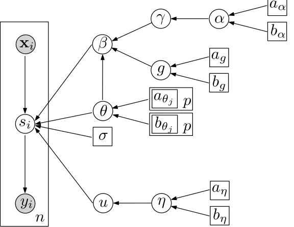
The corresponding directed acyclic graph is shown in Figure 1.

s

x

y

u

σ

β

η

a

b

n

g

a

b

α

a

b

γ

θ

a

b

p

p

Figure 1: A graphical representation for the hierarchical model.

3.2 Inference

Our goal is to generate realizations of parameters from the conditional joint density p(s,u,β,γ,g|y) via an MCMC algorithm. In order to speed up mixing of the MCMC, we use marginal posterior distributions whenever possible. Our MCMC algorithm consists of the following steps.

Start Give aη, bη, agand bg, and initialize s,γ, g,η, u andβ_γ.

Step (a) Impute each sifrom p(si|yi,u,β_γ).

Step (b) Updateη, g, eβ_γandθaccording to p(η|u), p(g|β_γ), p(eβ_γ|s,γ,η,g) and p(θ|s,γ), respec-tively.

Step (a) is to draw s from p(s|y,u,β_γ). We perform this step by using a technique which was pro-posed by Holmes and Held (2006) for the conventional probit regression. In particular, s is updated from its marginal distribution having integrated over ˜β_γ; that is, si is generated from p(si|s−i,yi,γ)

where s−i= (s1, . . . ,si−1,si+1, . . . ,sn)′. The details of this procedure is given in Appendix A. Please

also refer to Holmes and Held (2006).

We now consider the updates of eβ_γ, η and g. Given s, these parameters are independent

of y, so their updates are based on p(eβ_γ,η,g|s,γ). Hence, we update eβ_γ from [eβ_γ|s,γ,η,g]∼

Nnγ+1(ϒ−_γ1Ke′_γs,ϒ−_γ1). Since g is only dependent onβ_γand the prior is conjugate, we use the Gibbs sampler to update g from its conditional distribution, which is given by

[g|β_γ]∼Ga

_ag+nγ

2 ,

bg+β′_γKγγβ_γ

2

.

The update ofηis obtained from its conditional distribution as

[η|u]_∼Ga

_aη+1

2 ,

b_η+u2 2

.

In order to updateθ, we need to use an MH sampler. We write the marginal conditional distri-bution ofθas

p(θ|s,γ)∝p(s|γ,η,g,θ)p(θ),

where p(s|γ,η,g,θ) is given by (8). In the following experiments (see Section 5.3), the proposal distribution is specified as a Gaussian distribution with the current value ofθas mean and 0.2 as

variance. Letθ∗ denote the proposed move from the current θ. Then this move is accepted with

probability

min

n

1, p(s|γ,η,g,θ ∗₎

p(s|γ,η,g,θ)

o

.

This acceptance probability involves the calculations of the inverses and determinants of both Qγ and Q∗_γ, where Q∗_γ is obtained from Q_γ with θ∗ replacingθ. To reduce computational costs, we employ the formulas in (11) which is given below for computing these inverses and determinants.

Our Bayesian estimation method for the kernel parameter θ is more efficient than that given in

BSVM and CSVM (Mallick et al., 2005), in which computing the inverses and determinants of two

consecutive full kernel matrices K and K∗is required at each sweep of MCMC sampling.

Step (c) is used for the automatic choice of active vectors. To implement this step, we borrow a method devised by Nott and Green (2004). This method was derived from the reversible jump methodology of Green (1995). Specifically, we generate a proposalγ∗from the current value ofγ by one of three possible moves:

Birth move randomly choose a 0 inγand change it to 1;

Death move randomly choose a 1 inγand change it to 0;

Swap move randomly choose a 0 and a 1 inγand switch them.

The acceptance probability for each move is

Letting k=nγ, we denote the probabilities of birth, death and swap by bk, dk and 1−bk−dk,

respec-tively. For birth, death and swap moves, the acceptance probabilities are

min

1,p(s|γ

∗_)p(γ∗_)d

k+1(n−k) p(s|γ)p(γ)bk(k+1)

,

min

1, p(s|γ

∗_)p(γ∗_)b k−1k p(s|γ)p(γ)dk(n−k+1)

,

min

1,p(s|γ ∗_)p(γ∗₎

p(s|γ)p(γ)

,

where p(s|γ) and p(γ) are given in (8) and (10). In our experiments we set b0=1 and d0=0, bk=dk=0.3 for 1≤k≤kmax−1, and dk=1 and bk=0 for kmax≤k≤n. Here, kmaxis a specified

maximum number of active vectors such that kmax≤n.

An alternative to this approach is the stochastic search method of George and McCulloch (1997). This method also employs birth, death and swap moves; it differs from the reversible jump proce-dure because it does not incorporate the probabilities of birth, death and swap into its acceptance probabilities.

Recall that the main computational burden of our MCMC algorithm comes from the calculations of the determinant and inverse of Qγ(Qγ∗) during the MCMC sweeps. It is worth noting that when

n is relatively large, we can reduce the computational burden by giving kmaxa value far less than n, that is, kmax≪n, and then computing:

Q_γ−1=In−Keγϒγ−1Ke′γ and |Qγ|=|ϒγ||Σγ|−1=η−1g−nγ|Kγγ|−1|ϒγ|. (11)

For example, for both the USPS and NewsGroups data sets used in our experiments, we set kmax=

200≪n. In this setting, we always have n_γ≤kmax≪n. Sinceϒγ and Kγγ are(nγ+1)×(nγ+1) and nγ×nγ, these formulas for Q−_γ1 and|Qγ|are feasible computationally. This is an advantage over the stochastic search method of George and McCulloch (1997). Finally, in the reversible jump method, the matrices obtained before and after each move only change a column and a row. Thus, it is possible to exploit rank-one matrix update techniques to make the method still more efficient.

3.3 Prediction

Given a new input vector x∗, we need to predict its label y∗. The posterior predictive distribution of

y∗is

p(y∗|x∗,y) =

Z

p(y∗|x∗,β˜_γ,y)p(β˜_γ|y)d ˜β_γ.

We know that this integral cannot be computed in closed form. Moreover, it is intractable to select the model which is parameterized byβ_γfor prediction. An intuitive approach is to choose a model

with a value of γhaving the highest posterior probability among those γ that appear during the

MCMC sweeps. However, this is expensive in terms of memory becauseγtakes 2npossible distinct

values. To deal with this problem, we use a Bayesian model averaging method (Raftery et al., 1997) for posterior prediction.

The Bayesian model averaging method is based on the MCMC sampling process. Specifically, we have

p(y∗=1|x∗,y)≈ 1

T

T

∑

y∗=1

Here(·)(t)_{is the tth MCMC realization of(·), which is taken at every Mth sweep after the burn-in}

of the MCMC algorithm. In the following experiments, we run the MCMC algorithm for 10,000

sweeps, discard the first 5,000 as the burn-in, and retain every 5th (i.e., M =5) realization of parameters after the burn-in for inference and prediction. This implies that the Bayesian model averaging method uses 1,000 (T = (10,000−5,000)/5) active sets for prediction.

We should point out that our Bayesian model does not treat the training and test as two sep-arate procedures. In fact, our reversible jump MCMC algorithm deals with parameter estimation, model selection and posterior prediction jointly in a single paradigm. Moreover, the reversible jump method is a sequential approach for model selection and posterior prediction. This implies that after the burn-in the selection of active vectors and the prediction of responses are simultaneously im-plemented. Thus, the MCMC algorithm does not require extra computational complexity for the prediction of responses.

4. Sparse Gaussian Processes for Classification

In nonparametric Bayesian methods for regression and classification, f(x) is directly regarded as a stochastic function; in particular, f(x)is often modeling as a Gaussian process. There has been much discussion of the relationships between RKHS-based methods and GP-based methods (see, e.g., Rasmussen and Williams, 2006; Pillai et al., 2007). In this section we further investigate this relationship and then propose an effective and efficient GP-based classification method.

4.1 Gaussian Process Priors

The following proposition summarizes the connection between the Gaussian process and the feature basis expansion∑r_k=1bkψk(x)given in (4).

Proposition 1 Given a Gaussian process ζ(x) over

X

X

X

X

X

ζ(x) =

r

∑

bkψk(x) with bki∼.i.dN(0,g−1). (12)

Conversely, given a functionζ:

X

If the feature expansion in (12) is regarded as a stochastic process, it is known as the Karhunen-Lo`eve expansion. Proposition 1 provides a direct connection between GKMs and GP classifiers (GPCs) (Neal, 1999; Girolami and Rogers, 2006), and between GKMs and model-based geostatis-tics (Diggle et al., 1998). We see that b= (b1, . . . ,br)′ behaves as a regression vector in GKMs,

As discussed in Section 2, the Karhunen-Lo`eve expansion can also be approximated by a finite-dimensional expansion over the training data set; that is,

ζ(x) =

n

∑

βiK(x,xi) with β= (β1, . . . ,βn)′∼Nn(0,g−1K−1).

Letζ= (ζ(x1), . . . ,ζ(xn))′ be the vector of n realizations ofζover the training data. We then have ζ=Kβ∼Nn(0,g−1K). In our sparse treatment, some of theβiare set to zero and the subvectorβ_γ

of the nonzero elements is modeled as Nnγ(0,g−1Kγγ−1). In this case,ζ=Kγβγ follows a singular normal distribution, that is, ζ∼Nn(0,g−1KγK−_γγ1K′_γ). This sparse technique is called the

“sub-set of regressors” (Rasmussen and Williams, 2006). In the following sections we investigate this sparsity-inducing approach to GP-based classification as an alternative to the FBGKM introduced in Section 3.

4.2 The MCMC Algorithm

By analogy with on the hierarchical model for our FBGKM in Section 3.1, we model the auxiliary variable sias

si=s(xi) =u+ζ(xi) +εi with εi∼N(0,1)

and keep other settings unchanged. Here ζ(x) is the Gaussian process with E(ζ(x)) =0 and Cov(ζ(xi),ζ(xj)) =g−1K(xi,xj). Applyingζ(x)to the training data, we have

s=u1n+ζ+ε with ε∼Nn(0,In).

The inverses of n×n matrices are also required during Bayesian inference and prediction for GPCs. In order to reduce the computational costs, we use K_γβ_γ withβ_γ∼Nnγ(0,g−1K−γγ1)to

ap-proximate ζas in Section 4.1. This yields a sparse GPC (SGPC) model. The MCMC algorithm

for SGPC is immediately obtained from that for FBGKM by simply removing the update ofβ_γin

Section 3.2, becauseβ_γis now the latent vector and it is not used for prediction. In particular, GPCs use the expectation of y∗w.r.t. p(y∗|x∗,y)as the predictor. We thus need to insert a step, which is to

sample s∗=s(x∗)from p(s∗|s,γ,u,y), into the MCMC algorithm for prediction. This step is only

necessary at every Mth sweep after the burn-in of the MCMC algorithm (see Diggle et al., 1998). Now the marginal distribution of s is [s|u,γ]∼Nn(u1n, Mγ), where Mγ=In+g−1KγK−_γγ1K′_γ.

Since s∗is conditionally independent of y, given s, we have

p(s∗|s,γ,u) =N u+g−1kγ(x∗)′Kγγ−1K′γMγ−1(s−u1n),v

,

where v=g−1k_γ(x∗)′K−γγ1kγ(x∗)+1−g−2kγ(x∗)′K−γγ1K′γM−γ1KγK_γγ−1k_γ(x∗) and kγ(x∗) is the

sub-vector of(K(x∗,x1), . . . ,K(x∗,xn))′ corresponding toγi =1. Since we haveE(y∗|s∗) =τ(s∗)and

the used probit link τ is a monotonically increasing function on (−∞, ∞), we allocate y∗ =1 if

s∗>0 and y∗=0 otherwise.

Let

I

then v is near zero and the posterior predictive mean of s∗ reverts to u when x∗ is far from points

It is again worth noting that the reversible jump MCMC algorithm devised in this paper deals with parameter estimation and posterior prediction jointly in a single paradigm. Moreover, the reversible jump methodology is a sequential approach to model selection and posterior prediction. The main computational burden of the MCMC algorithm comes from the sampling procedure for parameter estimation, and the MCMC algorithm does not require extra computational complexity for the selection of active vectors and the prediction of responses.

The MCMC algorithms used in Neal (1999) and Diggle et al. (1998) is less efficient than ours because they do not use data augmentation or exploit sparsity. Girolami and Rogers (2006) proposed a Bayesian multinomial probit regression model, using variational methods for inference. For addi-tional discussion of sparse approaches to GPs, interested readers should refer to Qui˜nonero-Candela and Rasmussen (2005), Rasmussen and Williams (2006) and Snelson (2007) and references therein.

5. Experimental Evaluations

In this section we conduct several experiments to evaluate the performance of our proposed Bayesian classification methods: FBGKM and SGPC. We compare the methods with various closely re-lated Bayesian and non-Bayesian classification methods, including the Bayesian SVM (BSVM) (Mallick et al., 2005), the complete SVM (CSVM) (Mallick et al., 2005), sparse Gaussian processes (SGP+FIC) (Snelson and Ghahramani, 2006), and the conventional IVM and SVM.

We also implement our Bayesian GKM without Step (c) of the MCMC algorithm in Section 3.2. That is, we implement an MCMC algorithm that consists of Steps (a)-(b) by fixing n_γ=n. We denote the resulting model by BGKM to distinguish it from FBGKM. We could also implement a full (non-sparse) GPC, but since such a full GPC would have almost the same computational complexity as the GBKM, we do not implement the non-sparse GPC. All experiments have been implemented in Matlab on a Pentium 4 with a 2.80GHz CPU and 2.00GB of RAM.

5.1 Setup

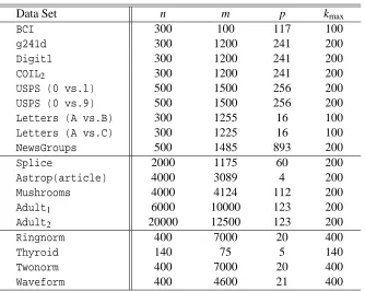
We perform the experiments on several benchmark data sets: BCI, g241d, Digit1, COIL₂, USPS

digits {(0 vs. 1), (0 vs. 9)}, Letters {(A vs. B), (A vs. C)}, NewsGroups corpora,

Adult₁, Adult₂, Mushrooms, Splice, Astroparticle, Ringnorm, Thyroid, Twonorm, and

Waveform. We first present a brief review of these data sets.

The BCIdata set contains data obtained from project in brain-computer interfaces in which a

single subject performs 400 trials in which he imagines movements with either the left or right hand. Theg241ddata set is an artificial data set which is generated by two unit-variance isotropic

Gaussians with potentially misleading cluster structure. The Digit1data set is generated by

ap-plying a sequence of transformations to digit images, leading to a low-dimensional manifold

ge-ometrical structure embedded into a high-dimensional space. TheCOIL₂ data set is derived from

the Columbia object image library (COIL-100) under a sequence of transformations, for example, rescaling, adding noise, and masking dimensions. Note that theBCI,g241d,Digit1andCOIL₂data

sets are available athttp://www.kyb.tuebingen.mpg.de/ssl-book/.

The USPS database is a handwritten digits data set which contains the digits from 0 to 9 auto-matically scanned from envelopes by the U.S. Postal Service. In our experiments, two digit pairs

{(0 vs. 1), (0 vs. 9)}data sets are randomly constituted from the USPS database, and the

“A” to “Z,” and two letter pairs{(A vs. B), (A vs. C)}are randomly constituted from “A,” “B” and “C” with 789, 766, and 736 cases, respectively.

The20 NewsGroupsdata set is organized into 20 different newsgroups, each corresponding to

a different topic, and we randomly select thealt.atheism andcomp.graphicstopics for the binary classification problem. The total vocabulary size is 1390. Based on the information gain, 893 features are employed.

The Adultdata set is originally extracted from the 1994 Census database with 14 features, of

which six features are continuous and eight are categorical. Further, theAdultdata set is processed with dimensionality of 123, that is, each continuous feature is discretized into a binary feature and each categorical feature with q categories is converted to q binary features. Here, theAdult₁and

Adult2data sets are constituted according to different training and test sizes.

The Mushrooms data set is originally drawn from the Audubon Society Field Guide to North

American Mushrooms with 22 features. Similar to the Adult data set, the Mushrooms data set

is processed into the binary feature representations, leading to 123 dimensions for each instance.

TheSplice data set is based on the biological process whereby intronic DNA is removed during

protein translation. TheAstrop (Astroparticle) data set is obtained from Jan Conrad of Uppsala

University, Sweden. TheAdult,Mushrooms,Splice, andAstropdata sets are available athttp:

//www.csie.ntu.edu.tw/˜cjlin.

The Ringnorm data set is artificially generated from two multivariate Gaussian distributions

for the binary classification problem. That is, the instances within each class are obtained from

a 20-variate Gaussian distribution. The Thyroid is collected from several databases of thyroid

disease records. We use this data set to conduct a binary classification experiment in which the class euthyroidism is considered as the normal class and the classes hypothyroidism and hyperthyroidism are considered as an abnormal class.

TheTwonormdata set is also an artificial 20-dimensional two-class classification example, which

consists of 7400 instances. TheWaveformdata set is generated from a combination of 2 of 3 “base”

waves in a 21-dimensional space. TheRingnorm,Thyroid,Twonorm, andWaveformdata sets are

widely used for the classification benchmarking, and they are available at http://ida.first.

gmd.de/˜raetsch/data/benchmarks.htm.

Table 1 gives a summary of these data sets. In our experiments, each data set is randomly partitioned into two disjoint subsets as the training and test. Twenty random partitions are gener-ated for each data set. Based on these partitions, several evaluation criteria, including the average classification error rate, standard deviation and average computational time, are reported.

All of the methods that we implement are based on a Gaussian RBF kernel with a single width parameter; that is, K(xi,xj) =exp −kxi−xjk2₂/θ2

. In Section 5.3 we present experiments in which this hyperparameter is estimated from data based on the ideas discussed in Section 3.2. In the remaining sections, however, we use a simpler procedure in which the value ofθis set to the mean Euclidean distance between training data points. We found this setting to be effective empirically in our applications. The gain in computational complexity is significant, particularly for the full GP methods, BSVM and CSVM, whose calculations involve two full kernel matrices. In particular, for each new value ofθ, it is necessary to recalculate the kernel matrix K for each sweep of the MCMC algorithms.

In addition, we set the hyperparameters in both FBGKM and SGPC as follows: a_η=1, b_η=

0.1, ag=4 and bg =0.1. For all of the Bayesian classification methods, we run each MCMC

Data Set n m p kmax

BCI 300 100 117 100

g241d 300 1200 241 200

Digit1 300 1200 241 200

COIL2 300 1200 241 200

USPS (0 vs.1) 500 1500 256 200

USPS (0 vs.9) 500 1500 256 200

Letters (A vs.B) 300 1255 16 100

Letters (A vs.C) 300 1225 16 100

NewsGroups 500 1485 893 200

Splice 2000 1175 60 200

Astrop(article) 4000 3089 4 200

Mushrooms 4000 4124 112 200

Adult₁ 6000 10000 123 200

Adult2 20000 12500 123 200

Ringnorm 400 7000 20 400

Thyroid 140 75 5 140

Twonorm 400 7000 20 400

Waveform 400 4600 21 400

Table 1: Summary of the Benchmark Data Sets: n—the size of the training data set; m—the size

of the test data set; p—the dimension of the input vector; kmax—the maximum number of

active vectors.

of parameters after the burn-in for inference and prediction. These settings are empirically validated to be sufficient for these methods to achieve convergence. Recall that the test is implemented after the burn-in of the MCMC sampling. This implies that the Bayesian model averaging component of our Bayesian methods uses 1,000 (T = (10,000−5,000)/5) active sets for test.

5.2 Evaluation 1

In the first evaluation, we compare BGKM, FBGKM and SGPC with BSVM and CSVM, because they are the two existing Bayesian kernel methods most closely related to our Bayesian classification methods.

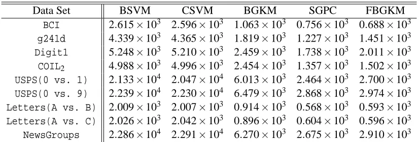
We conduct this evaluation on the first nine data sets in Table 1, randomly partitioning the data into disjoint training and test data sets according to the corresponding settings of n and m. All the inputs are normalized to have zero mean and unit variance. Tables 2 and 3 report the performance of the five Bayesian methods on the nine different data sets in terms of the average classification error rate (%), the standard deviation and the corresponding average computational time (s).

Data Set BSVM CSVM BGKM SGPC FBGKM err (±std) err (±std) err (±std) err (±std) err (±std)

BCI 28.15 (±2.15) 29.40 (±2.58) 29.35 (±2.82) 27.10 (±1.85) 29.83 (±2.36)

g241d 17.15 (±1.68) 17.63 (±1.15) 16.37 (±1.11) 16.55 (±1.22) 16.30 (±0.89)

Digit1 4.86 (±0.74) 4.88 (±0.75) 4.87 (±0.65) 5.51 (±0.66) 4.85 (±0.67)

COIL₂ 9.71 (±0.81) 9.86 (±0.71) 9.16 (±0.99) 9.83 (±0.97) 9.797 (±0.32)

USPS(0 vs. 1) 0.40 (±0.30) 0.35 (±0.11) 0.28 (±0.05) 0.31 (±0.14) 0.28 (±0.06)

USPS(0 vs. 9) 1.36 (±0.36) 1.40 (±0.29) 1.36 (±0.28) 1.21 (±0.19) 1.37 (±0.24)

Letters(A vs. B) 0.92 (±0.59) 0.95 (±0.45) 0.75 (±0.24) 0.53 (±0.19) 0.77 (±0.24)

Letters(A vs. C) 0.83 (±0.15) 0.93 (±0.27) 0.87 (±0.15) 0.65 (±0.20) 0.84 (±0.15)

NewsGroups 5.62 (±0.80) 5.08 (±0.33) 4.92 (±0.28) 4.66 (±0.38) 4.83 (±0.25)

Table 2: Experimental results for the five methods on different data sets: err−the test error rates (%); std−the corresponding standard deviation.

Data Set BSVM CSVM BGKM SGPC FBGKM

BCI 2.615×103 2.596×103 1.063×103 0.756×103 0.688×103

g241d 4.339×103 4.365×103 1.819×103 1.227×103 1.451×103

Digit1 5.248×103 _5.210×103 _2.459×103 _1.738×103 _2.011×103

COIL2 4.988×103 4.996×103 2.454×103 1.357×103 1.502×103

USPS(0 vs. 1) 2.133×104 2.047×104 6.013×103 2.464×103 2.700×103

USPS(0 vs. 9) 2.239×104 2.230×104 6.479×103 2.868×103 2.974×103

Letters(A vs. B) 2.009×103 2.007×103 0.914×103 0.568×103 0.593×103

Letters(A vs. C) 2.026×103 2.042×103 0.896×103 0.604×103 0.596×103

NewsGroups 2.286×104 2.291×104 6.270×103 2.675×103 2.910×103

Table 3: The computational times (s) for the five methods on different data sets.

In the following experiments, we attempt to analyze the performance of the methods with respect to different values of the training size n and the maximum number kmax of active vectors. For the

sake of simplicity, we only report results on theNewsGroupsdata set.

Tables 4 and 5 show the experimental results when changing the training size n and fixing the

maximum number of active vectors to kmax=200. As can be seen, all the five methods obtain a

lower classification error rate and have greater computational costs as the training size n increases. Furthermore, FBGKM, SGPC and BGKM slightly outperform BSVM and CSVM in both classi-fication error rate and computational cost. The FBGKM and SGPC methods are relatively more efficient for the data sets of large training size n.

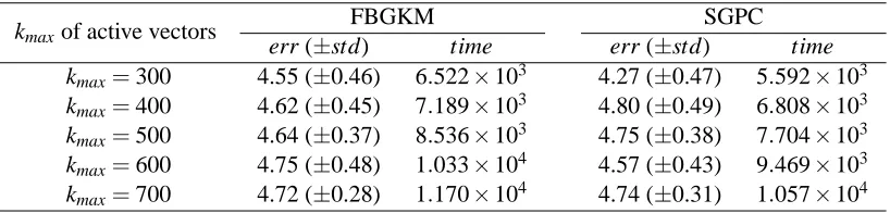
Table 6 shows the experimental results for our FBGKM and SGPC methods with respect to

different values of the maximum number kmax of active vectors and for a fixed training size of

n=800. The performance of these two methods is roughly similar for each setting kmax; that is,

they are insensitive to kmax. However, their computational costs tend to slightly increase as the

maximum number kmaxof active vectors increases.

Training size n BSVM CSVM BGKM SGPC FBGKM err (±std) err (±std) err (±std) err (±std) err (±std)

n=300 5.99 (±1.44) 5.84 (±0.80) 5.37 (±0.52) 5.34 (±0.40) 5.08 (±0.49)

n=400 5.65 (±0.98) 5.83 (±0.93) 5.10 (±0.35) 5.03 (±0.55) 5.05 (±0.39)

n=500 5.62 (±0.80) 5.08 (±0.33) 4.92 (±0.28) 4.66 (±0.38) 4.83 (±0.25)

n=600 5.77 (±0.61) 5.13 (±0.20) 4.92 (±0.43) 4.35 (±0.47) 4.74 (±0.28)

n=700 5.63 (±0.82) 4.82 (±0.21) 4.44 (±0.36) 4.12 (±0.22) 4.61 (±0.52)

n=800 5.14 (±0.59) 5.10 (±0.16) 4.49 (±0.47) 4.13 (±0.51) 4.56 (±0.34)

Table 4: Experimental results for the five methods corresponding to different training sizes n on the

NewsGroupsdata set with kmax=200: err−the test error rates (%); std−the

correspond-ing standard deviation.

Training size n BSVM CSVM BGKM SGPC FBGKM

n=300 5.949×103 5.830×103 2.467×103 1.862×103 2.085×103

n=400 1.173×104 _1.171×104 _4.674×103 _2.555×103 _2.804×103

n=500 2.286×104 2.291×104 6.270×103 2.675×103 2.910×103

n=600 3.458×104 3.461×104 8.340×103 2.748×103 2.973×103

n=700 5.195×104 _5.186×104 _1.207×104 _3.279×103 _3.610×103

n=800 7.754×104 7.757×104 1.673×104 3.885×103 4.327×103

Table 5: The computational times (s) for the five methods corresponding to different training sizes n on theNewsGroupsdata set with kmax=200.

kmaxof active vectors

FBGKM SGPC

err (±std) time err (±std) time

kmax=300 4.55 (±0.46) 6.522×103 4.27 (±0.47) 5.592×103

kmax=400 4.62 (±0.45) 7.189×103 4.80 (±0.49) 6.808×103

kmax=500 4.64 (±0.37) 8.536×103 4.75 (±0.38) 7.704×103

kmax=600 4.75 (±0.48) 1.033×104 4.57 (±0.43) 9.469×103

kmax=700 4.72 (±0.28) 1.170×104 4.74 (±0.31) 1.057×104

Table 6: Experimental results for FBGKM and SGPC corresponding to different maximum num-bers kmax of active vectors on theNewsGroupsdata set with n=800: err−the test error

rates (%); std−the corresponding standard deviation; time−the corresponding computa-tional time (s).

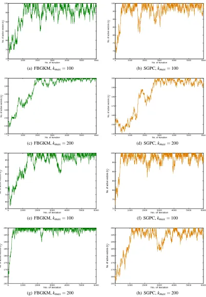
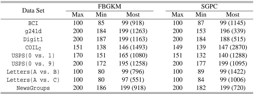
depicts the output of the numbers n_γof active vectors corresponding to the first 6000 sweeps in the

MCMC inference procedure onBCI,Digit1,Letters{(A vs.B)}andNewsGroups. The results

0 1000 2000 3000 4000 5000 6000 70 75 80 85 90 95 100

No. of iteration

No. of active vectors (n

γ

)

(a) FBGKM, kmax=100

0 1000 2000 3000 4000 5000 6000

65 70 75 80 85 90 95 100

No. of iteration

No. of active vectors (n

γ

)

(b) SGPC, kmax=100

0 1000 2000 3000 4000 5000 6000

130 140 150 160 170 180 190 200

No. of iteration

No. of active vectors (n

γ

)

(c) FBGKM, kmax=200

0 1000 2000 3000 4000 5000 6000

140 150 160 170 180 190 200

No. of iteration

No. of active vectors (n

γ

)

(d) SGPC, kmax=200

0 1000 2000 3000 4000 5000 6000

60 65 70 75 80 85 90 95 100

No. of active vectors (n

γ

)

No. of iteration

(e) FBGKM, kmax=100

0 1000 2000 3000 4000 5000 6000

70 75 80 85 90 95 100

No. of active vectors (n

γ

)

No. of iteration

(f) SGPC, kmax=100

0 1000 2000 3000 4000 5000 6000

160 165 170 175 180 185 190 195 200

No. of iteration

No. of active vectors (n

γ

)

(g) FBGKM, kmax=200

0 1000 2000 3000 4000 5000 6000

160 165 170 175 180 185 190 195 200

No. of iteration

No. of active vectors (n

γ

)

(h) SGPC, kmax=200

Figure 2: MCMC Output for the numbers n_γ of active vectors of our FBGKM and SGPC

meth-ods on the four data sets: (a/b) BCI; (c/d) Digit1; (e/f) Letters (A vs. B); (g/h)

In probit-type models, since the posterior distribution of each si is truncated normal, we are

able to update the si using the Gibbs sampler. Recall that we employ an efficient auxiliary variable

approach proposed by Holmes and Held (2006) for the implementation of the Gibbs sampler (see

Appendix A). For the other models, however, a MH sampler is required to update the si. This

makes the corresponding MCMC algorithms take longer to mix. Thus, our models, which are based on the probit link, can be expected to be more efficient computationally than the BSVM and CSVM. However, to standardize the experimental comparison, we use the same setup for MCMC sweeps and burn-in for all algorithms.

Table 7 describes distributions of active vectors to appear after the burn-in (in the last 5,000 sweeps). As we can see, the number n_γof active vectors jumps between a small range for different data sets, due to the rapid mixing. The maximum frequency of active vectors corresponding to the number n_γof active vectors is also given in Table 7.

Data Set FBGKM SGPC

Max Min Most Max Min Most

BCI 100 85 99 (918) 100 87 99 (1145)

g241d 200 184 199 (1263) 200 153 196 (339)

Digit1 200 187 199 (1163) 200 184 188 (515)

COIL₂ 151 138 146 (1493) 149 139 147 (2870)

USPS(0 vs. 1) 170 151 165 (1080) 151 132 140 (1288)

USPS(0 vs. 9) 200 172 195 (1258) 200 177 199 (1095)

Letters(A vs. B) 100 80 99 (796) 100 89 99 (1422)

Letters(A vs. C) 100 80 97 (551) 100 84 99 (1006)

NewsGroups 200 186 199 (918) 200 182 199 (720)

Table 7: Distributions of active vectors after the burn-in under FBGKM and SGPC. Max—the max-imum number of active vectors to appear; Min—the minmax-imum number of active vectors to appear; Most—the number of active vectors with the maximum frequency and the corre-sponding frequency shown in brackets.

5.3 Evaluation 2

We further evaluate the performance of our sparse Bayesian kernel methods under kernel parameter learning, and compare the FBGKM and SGPC with SGP+FIC and full GP (FGP) (Rasmussen and Williams, 2006). In particular, we use the Gaussian RBF kernel with multiple parameters, that is, K(xi,xj) =exp −∑_lp₌₁(xil−xjl)2/θ2l

, and estimate those parameters θ= (θ1, . . . ,θp) in all

compared Bayesian kernel methods. In order to distinguish from the Bayesian methods with the

fixed kernel parameters, we label the Bayesian methods with the learned parameters via “⋆+KL.”

We conduct experimental analysis on the Adult, Mushrooms, Splice, andAstroparticle data

sets.

Since for FGP+KL learning the kernel parameters results in a huge computational cost, we set the sizes of the training and test data as 1000 (i.e., n=m=1000) in each data set. In this setting,

there is no distinction between Adult1 and Adult2, so we just use Adult to denote the

expectation propagation (EP) algorithm (Minka, 2001) for FGP+KL. However, to provide an apples-to-apples comparison with our sparse Bayesian kernel methods, we employ MCMC inference for SGP+FIC+KL. For the sparse methods compared here, we fix the size of active set to 100, that is,

kmax=100. Our implementations for SGP+FIC and FGP are based on the Matlab codes fromhttp:

//www.lce.hut.fi/research/mm/gpstuff/andhttp://www.gaussianprocess.org/gpml/,

respectively.

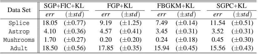
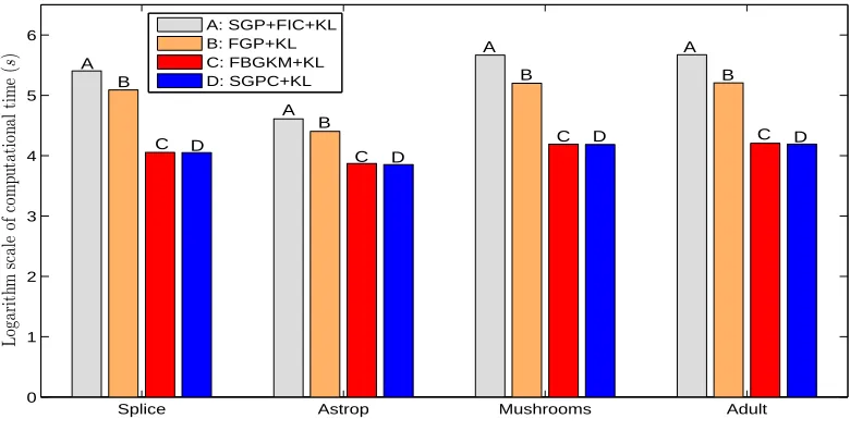
Tables 8 and 9 and Figure 3 report the performance of the SGP+FIC+KL, FGP+KL, FBGKM+KL, and SGPC+KL methods on the four data sets in terms of the average classification error rate (%), the standard deviation and the corresponding average computational time (s). Figure 3 depicts the logarithm scale of the corresponding average computational time (s) on the different data sets. It is clear that FBGKM+KL and SGPC+KL outperform other methods on the whole. Additionally, the computational times of all compared methods tend to increase when the number p of the kernel parameters increases. We note that the computational times of SGP+FIC+KL and FGP+KL would become huge if we directly applied them to the large data sets listed in Table 1—Adult₁,Adult₂,

Mushrooms,Splice, andAstroparticle.

Data Set SGP+FIC+KL FGP+KL FBGKM+KL SGPC+KL

err (±std) err (±std) err (±std) err (±std)

Splice 18.05 (±0.77) 9.19 (±1.25) 7.49 (±0.14) 11.54 (±0.51)

Astrop 4.10 (±0.36) 4.57 (±0.41) 3.45 (±0.31) 3.52 (±0.31)

Mushrooms 1.70 (±0.27) 0.20 (±0.20) 0.24 (±0.18) 0.45 (±0.30)

Adult 18.50 (±0.56) 17.85 (±0.35) 15.94 (±0.45) 15.56 (±0.43)

Table 8: Experimental results for the four Bayesian kernel methods on the four data sets with

learned kernel parameters θ, kmax=100, n=1000, and m=1000: err−the test error

rates (%); std−the corresponding standard deviation.

Data Set SGP+FIC+KL FGP+KL FBGKM+KL SGPC+KL

Splice 2.542×105 1.228×105 1.132×104 1.121×104

Astrop 4.081×104 2.531×104 7.431×103 7.103×103

Mushrooms 4.639×105 1.583×105 1.551×104 1.534×104

Adult 4.713×105 1.605×105 1.606×104 1.557×104

Table 9: The computational times (s) of the four Bayesian kernel methods on the four data sets with learned kernel parametersθ, kmax=100, n=1000, and m=1000.

In order to further evaluate the performance of our sparse Bayesian kernel methods on some larger data sets, we also conduct comparative experiments of FBGKM, SGPC, and SGP+FIC

(Snel-son and Ghahramani, 2006) on theAdult₁,Adult₂,Mushrooms,Splice, andAstroparticledata

Splice Astrop Mushrooms Adult 0

1 2 3 4 5 6

L

og

ar

it

hm

sc

al

e

of

co

m

pu

ta

ti

on

al

ti

m

e

(

s

)

A: SGP+FIC+KL B: FGP+KL C: FBGKM+KL D: SGPC+KL

C

A B

C D

A B

C D

B

C D

B

A A

D

Figure 3: The computational times (s) for the four Bayesian kernel methods on the four data sets with learned kernel parameterθ, kmax=100, n=1000, and m=1000.

Table 10 reports the classification performance of the SGP+FIC+MCMC, SGP+FIC+EP, FBGKM and SGPC methods on the five data sets. It should be pointed out here that we do not report the

cor-responding results of SGP+FIC+MCMC on theAdult2data set due to the huge computational times

of performing it on this data set. From Table 10, we can see that our FBGKM and SGPC methods outperform other methods on the whole. Furthermore, it is still difficult for SGP+FIC+MCMC and SGP+FIC+EP to calculate the optimal solution for sparse approximation of full Gaussian process, due to the sensitivity of the performance to the initial active set.

Data Set SGP+FIC+EP SGP+FIC+MCMC FBGKM SGPC SVM

err (±std) err (±std) err (±std) err (±std) err (±std)

Splice 14.38 (±1.10) 16.32 (±0.15) 12.53 (±0.57) 12.07 (±0.45) 13.01 (±0.69)

Astrop 5.20 (±0.26) 3.38 (±0.11) 3.59 (±0.18) 3.34 (±0.16) 3.37 (±0.14)

Mushrooms 1.55 (±0.21) 1.38 (±0.13) 0.19 (±0.08) 0.21 (±0.06) 0.55 (±0.37)

Adult₁ 15.89 (±0.38) 15.79 (±0.26) 15.24 (±0.21) 15.59 (±0.16) 16.64 (±0.33)

Adult₂ 15.49 (±0.21) − − 15.01 (±0.17) 15.26 (±0.19) 16.27 (±0.28)

Table 10: Experimental results for the five methods on theSplice,Astroparticle,Mushrooms,

Adult₁, andAdult₂ data sets with kmax=200: err−the test error rates (%); std−the

corresponding standard deviation.

Splice Astrop Mushrooms 0 1 2 3 4 5 6 7 Lo ga ri th m sc al e of co m pu ta ti on al ti m e ( s ) A: SGP+FIC+EP B: SGP+FIC+MCMC C: FBGKM D: SGPC Adult

1 Adult2

B

D C

D C D

B

C D

D C

A

A C A A

A B

B

Figure 4: The computational times (s) of the four sparse Bayesian kernel methods on theSplice,

Astroparticle,Mushrooms,Adult1, andAdult₂data sets with kmax=200.

other methods on the five different data sets, and that the computational times of SGP+FIC+EP, FBGKM and SGPC are very close to each other.

Data Set SGP+FIC+EP SGP+FIC+MCMC FBGKM SGPC

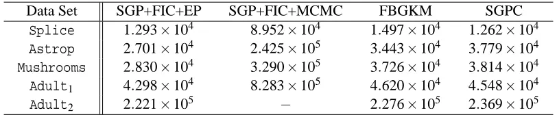
Splice 1.293×104 8.952×104 1.497×104 1.262×104

Astrop 2.701×104 _2.425×105 _3.443×104 _3.779×104

Mushrooms 2.830×104 3.290×105 3.726×104 3.814×104

Adult₁ 4.298×104 8.283×105 4.620×104 4.548×104

Adult₂ 2.221×105 _{− 2.276×10}5 _2.369×105

Table 11: The computational times (s) of the four sparse Bayesian kernel methods on theSplice,

Astroparticle,Mushrooms,Adult₁, andAdult₂data sets with kmax=200.

Data Set SGP+FIC+MCMC FBGKM SGPC

time burn-in time burn-in time burn-in

Splice 4.017×104 4566 1.019×103 906 2.195×103 1898

Astrop 9.265×104 _{3874 7.016×10}3 _{2125 1.123×10}4 ₃₂₁₈

Mushrooms 9.857×104 3192 1.362×104 3924 9.677×103 2616

Adult₁ 1.865×105 2451 8.605×103 1906 1.206×104 2873

Adult₂ − − 5.217×104 _{2424 8.142×10}4 ₃₆₀₅

Table 12: Monitoring convergence of MCMC algorithms for the three sparse Bayesian kernel

meth-ods on the Splice, Astroparticle, Mushrooms, Adult₁, and Adult₂ data sets with

kmax=200: time−the computational time (s) for convergence; burn-in−the length of

chain for convergence.

5.4 Bayesian vs. Non-Bayesian

Since FBGKM and SGPC are Bayesian alternatives to IVM and SVM, it is useful to compare our FBGKM and SGPC with the conventional IVM and SVM. We compared these methods on

the following data sets: Ringnorm, Thyroid, TwonormandWaveform. These data sets were also

used by Zhu and Hastie (2005) and a detailed presentation of results can be found in R¨atsch et al. (2001). Each data set is randomly partitioned into two disjoint subsets as training and test data sets according to the training and test sizes n and m given in Table 1. In addition, the maximum number kmax of active vectors is set according to Table 1. The results in Table 13 are based on the average

of twenty realizations and the results with the conventional IVM and SVM are cited from Zhu and Hastie (2005). We also conduct a comparison of FBGKM and SGPC with the conventional SVM on

theSplice,Astroparticle,Mushrooms,Adult1, andAdult2data sets. The classification results

are given in Table 10. From Tables 10 and 13 we can see that the Bayesian approaches slightly outperform the non-Bayesian approaches.

Data Set SVM IVM FBGKM SGPC

err (±std) err (±std) err (±std) err (±std)

Ringnorm 2.03 (±0.19) 1.97 (±0.29) 1.51 (±0.10) 1.56 (±0.12)

Thyroid 4.80 (±2.98) 5.00 (±3.02) 4.60 (±2.65) 4.51 (±2.32)

Twonorm 2.90 (±0.25) 2.45 (±0.15) 2.86 (±0.21) 2.79 (±0.23)

Waveform 9.98 (±0.43) 10.13 (±0.47) 9.80 (±0.31) 9.73 (±0.30)

Table 13: Experimental results for the four methods on the four data sets: err−the test error rates (%); std−the corresponding standard deviation.

6. Extensions

conditional likelihood from the hinge loss (also see Sollich, 2001) and assign a mixture of the point-mass distribution and the Silverman g-prior to the regression vector. In the following subsections we consider two additional extensions.

6.1 Multiple Kernel Learning

Kernel learning has emerged as an important theme in the machine learning community. We have provided a Bayesian foundation for kernel learning in Section 3. In particular, given a kernel func-tion, we can estimate parameters of the kernel function. We now discuss how to extend this capa-bility to the learning of combinations of kernels; the multiple kernel learning problem (Bach et al., 2004).

Assume that we are given q distinct kernel functions Kl(xi,xj), for l=1, . . . ,q. Correspondingly,

we have q feature functions (sayψ_l(x)). In this case, the predictive function is expressed as

f(x) =u+

q

∑

ψl(x)′bl.

Letting bl =glΨ′lβlwhereΨl= [ψl(x1), . . . ,ψl(xn)]′,βl = (βl1, . . . ,βln)′and gl≥0, we have

f(x) =u+

q

∑

gl n

∑

Kl(x,xi)βli.

Now we assignβ_l∼Nn 0,σ2(K(l))−1

and

gl ∼ρδ0(gl) + (1−ρ)Ga(gl|ag/2,bg/2),

where K(l)=ΨlΨl′(n×n) is the lth kernel matrix,δ0(·)is a point-mass at zero and the user-specific parameter ρ∈(0,1) controls the levels of the nonzero gl. Thus, we only need to update the gl

instead of g in the Bayesian computation in Section 3. Note that kernel parameter learning and multiple kernel learning can be incorporated together.

6.2 Multi-class Learning

We consider the extension of our fully Bayesian modeling approach to a c-class (c>2) classification problem where the class label yi is a binary c-vector with values all zero except a one in position j

if xibelongs to the jth class. In this case, we define c regression vectorsβj= (β1 j, . . . ,βn j)′∈Rn and c auxiliary vectors sj= (s1 j, . . . ,sn j)′∈Rn, j=1, . . . ,c, for each class. We then have

sj=1nuj+Kβj+ej, j=1, . . . ,c,

where the ej are i.i.d. from Nn(0,In).

We now denote u= (u1, . . . ,uc)′, B= [β1, . . . ,βc], S= [s1, . . . ,sc]and E= [e1, . . . ,ec]. As in the

binary problem, we also introduce a binary n-vectorγwith eitherγi=1 if xi is an active vector or γi=0 if xiis not an active vector. Let K′_γand Bγbe K′and B with the rows for whichγi=0 deleted.

Thus, we can form the following sparse model: