Mutual Information Based Matching for Causal Inference
with Observational Data
Lei Sun [email protected]
Department of Industrial and Systems Engineering University at Buffalo, Buffalo, NY 14260, USA
Alexander G. Nikolaev [email protected]
Department of Industrial and Systems Engineering
University at Buffalo, 312 Bell Hall, Buffalo, NY 14260, USA Department of Computer Science and Information Systems University of Jyvaskyla, Jyvaskyla, FIN-40014, Finland
Editor:Peter Spirtes
Abstract
This paper presents an information theory-driven matching methodology for making causal inference from observational data. The paper adopts a “potential outcomes framework” view on evaluating the strength of cause-effect relationships: the population-wide average effects of binary treatments are estimated by comparing two groups of units – the treated and untreated (control). To reduce the bias in such treatment effect estimation, one has to compose a control group in such a way that across the compared groups of units, treatment is independent of the units’ covariates. This requirement gives rise to a subset selection / matching problem. This paper presents the models and algorithms that solve the match-ing problem by minimizmatch-ing the mutual information (MI) between the covariates and the treatment variable. Such a formulation becomes tractable thanks to the derived optimality conditions that tackle the non-linearity of the sample-based MI function. Computational experiments with mixed integer-programming formulations and four matching algorithms demonstrate the utility of MI based matching for causal inference studies. The algorithmic developments culminate in a matching heuristic that allows for balancing the compared groups in polynomial (close to linear) time, thus allowing for treatment effect estimation with large data sets.
Keywords: Observational Causal Inference, Mutual Information, Matching, Subset Se-lection, Optimization
1. Introduction
The most widely adopted conventional matching methods employ various distance met-rics (e.g., Mahalanobis distance) and propensity scores (see Section 2 for a detailed review); the success of a matching venture is typically assessed by checking if the compared groups are “well-balanced”, i.e., if the distributions of covariates within them are similar. The methods introduced more recently strive to directly optimize balance (Zubizarreta, 2012). In particular, Nikolaev et al. (2013) re-cast matching as a subset selection problem with the objective to optimize a measure of covariate balance across groups (as opposed to indi-vidual unit pairs). The approach was coined Balance Optimization Subset Selection, with its applicability illustrated by employing linear programming models (Nikolaev et al., 2013) and simulated annealing heuristics (Tam Cho et al., 2013).
Note, however, that improving balance, expressed via some metric(s) capturing the dif-ference between the distributions of covariates in the compared groups, is just one approach that defines a matching procedure objective. It is as good as any other approach that would achieve the reduction of the dependence between the covariates and the treatment variable in the matched groups. This observation is exploited in the present paper, as it explores a new form of covariate balance and an alternative approach to doing matching.
This paper frames matching as an optimization problem with a mutual information (MI) based objective. The presented methods are non-parametric, and hence, do not suffer from human bias in model selection. The value of information theory in empirical statistics research and computer science has been emphasized over the past decade (Burnham and Anderson, 2002). However, while this thrust has been successful in facilitating hypothesis testing, optimization problems with information measures have proven to be difficult, mainly due to the inherent non-linearity of entropy and MI functions (Shannon, 1948). This paper presents a way to treat such non-linearity in subset selection problems, which arise in applying information theory logic for making causal inference with observational data.
MI has been used to formulate various problems involving feature selection (Est´evez et al., 2009), dependency analysis (Kraskov et al., 2004) and chaotic data identification (Fraser and Swinney, 1986). It measures the level of dependence between random variables; e.g., when evaluated for two variables, it takes a high value when one random variable con-tains much information about the other, signifying high dependence, while zero MI implies that the variables are independent. We show that the difference between the covariate dis-tributions among the treated and untreated units can be directly evaluated MI, exploiting the fact that randomization in treatment assignment implies zero MI between covariates and the treatment variable. To the best of the authors’ knowledge, no MI based method has yet been employed for grouping observations (units) to achieve a particular group property – most likely due to the non-linearity in the expression defining MI. This paper tackles this challenge and offers the models and algorithms that make theoretical and practical advances in subset selection, or simply, matching for treatment effect estimation.
First, this paper identifies pathways for the effective use of information theoretic mea-sures (namely, MI) in optimization problems. The presented theoretical analysis techniques for treating non-linearity are generic, and hence, can be adopted in other applications, where making assumptions on model/data structures is undesirable. More generally, this paper may open up venues for the application of mathematical programming and optimization techniques in information theory itself.
Second, this paper explains how MI can serve as the basis of a new form of covariate balance. The resulting MI-based matching method for selecting control groups for causal inference is flexible in that it can achieve solutions of pre-specified quality, with pre-set control group size, – moreover, it can optimize the latter. The presented algorithmic devel-opments produce a matching heuristic that runs in polynomial (close to linear) time: it thus allows for causal effect estimation with large data sets that are nowadays becoming available through mining social networks, health records, etc. While this work is not the first effort to employ the information theoretic tools for the needs of causal inference Hainmueller (2012), it appears to be the first where mutual information is used as an optimization objective.
The paper is organized as follows. Section 2 explains the problem of causal inference with observational data, and motivates optimization-driven subset selection approaches to attacking it. Section 3 introduces a class of MI-based matching problems with different ob-jectives. Section 4 derives optimality conditions for matched groups using MI, and presents the mixed integer programming-based and sequential selection-based matching algorithms that work to balance the covariate distributions across the treatment and control groups. Section 5 showcases the practical value of the MI-based matching approach by comparing the designed algorithms’ performance against the best previously existing matching meth-ods. Section 6 discusses the MIM limitations and future research directions. Section 7 provides concluding remarks and discusses the promising extensions of this line of work.
2. Causal Inference with Observation Data
Observational studies are often the only source of information about a program, policy, or treatment. For example, people non-randomly choose to participate in economy-boosting programs, political movements, online activities such as post re-tweeting, question answer-ing, service subscription, etc. In estimating any causal effect with such data, the researchers resort to the nonparametric data preprocessing, commonly referred to as matching (Ho et al., 2011).
Among different types of matching recipes, the first proposed and well-used one is the nearest neighbor matching (Rubin, 1973). It prescribes to pair up each observed treatment unit with a control unit so as to minimize a weighted distance between the units’ covariate vectors in each such pair. Mahalanobis distance is widely used for this purpose (Rubin, 1980), however, as a measure of divergence, it relies on elliptical distributions of covariates (Sekhon, 2008). Another widely-used recipe prescribes to match units on propensity score (Rosenbaum and Rubin, 1983) defined as the probability of a unit to receive treatment.
The Mahalanobis distance and propensity score based matching methods can be com-bined in various ways (Rubin, 2001; Diamond and Sekhon, 2013). However, such methods require assumptions on model and/or data structure. As such, true units’ propensity score values are generally unknown, and must be estimated via regression on covariates, which makes room for the researcher’s bias in data analysis (when one can “tinker with” with an analysis tool to make it output the result that one anticipates, perhaps subconsciously). This weakness has led to controversial exchanges between the authors analyzing the same data and reaching conflicting conclusions (Dehejia and Wahba, 1999, 2002; Smith and Todd, 2005b; Dehejia, 2005; Smith and Todd, 2005a).
Both the Mahalanobis distance and propensity score based matching methods are ap-plied with the objective to minimize the differences between the units in the treatment group and the control group of the same size. In contrast, Iacus et al. (2012) introduce a new class of matching methods, the Monotonic Imbalance Bounding (MIB) matching, which looks to assemble matched control groups consisting of a sufficiently large number of observations with a fixed pre-set level of maximum allowed imbalance. Based on the imbalance level, an algorithm is designed to split the range of each covariate into several coarse categories, so that any exact matching algorithm can be applied to solve this discretized problem.
Methodologies for direct optimization of balance have been proposed by researchers just recently. Rosenbaum et al. (2007) introduce a fine balance method, where exact balance is sought on several categorized nominal covariates and approximate matching is conducted on the remaining ones. For the exact matching part, a matrix of Mahalanobis distance values across all pairs of treatment and control units is defined, and then the classic assignment algorithm is used to minimize the total distance. Nikolaev et al. (2013) introduce Balance Optimization Subset Selection (BOSS) approach, optimizing explicit measures of balance and treating several models with exact and heuristic methods. Zubizarreta (2012) builds mixed integer programming models to optimize covariate balance directly by minimizing the total sum of the distances between the treated units and matched control units. The latter two lines of research work to measure the difference between the covariate distributions in the treatment group and control pool by employing chi-square, correlations, quantiles and Kolmogorov-Smirnov statistics, which are fundamentally different from the information theory-driven approach developed in the present paper.
3. Problem Definition
3.1 Motivating the Use of Matching for Causal Inference: Problem Statements
Given a set of observed units that have been treated, termed a treatment pool, and a set of observed untreated units, termed a control pool C, the causal inference problem objective is to evaluate the degree of influence of the treatment on the population units, termed treatment effect. For an observable unitu, letYu1(Yu0) denote a treated (untreated) response and tu a treatment indicator (1 means treated, 0 means not treated). Per Rubin’s model
of causal inference, these responses are referred to aspotential outcomes, reflecting the fact that it is impossible to observe bothYu1andYu0on the same unitu(Holland, 1986). For this reason, in estimating the population-wide effects of a treatment, researchers have to resort to comparing the averages across the treatment and control groups (Holland, 1986). One commonly targeted quantity of interest in causal inference studies, and the one this paper focuses on, is the average treatment effect for the treated (ATT),E(Y1|t= 1)−E(Y0|t= 1),
i.e., the average effect of treatment on the units that actually receive it.
Assume that a treatment group, T : |T | < |C|, is given (randomly selected from a treatment pool), so E(Y1|t = 1) can be estimated directly. A decision has to be made about selecting a control subsetS ⊂ Cso that the units inT andS can be compared. If the two groups have the same distribution of covariates, one can use the valueE(Y0|t= 0) over
S as an estimate of E(Y0|t = 1) over the entire population (refer Rosenbaum and Rubin (1983) for more statistical fundamental work), and then, obtain an estimate of ATT.
The goal of a matching procedure is to ensure that the covariate distributions in the treatment and control groups are as similar as possible. The key insight this paper exploits is that, if a matching procedure is successful, then it should make it impossible to distinguish the treatment units from the control units based on the covariates, or, in other words, learn the treatment status of an observation based on the information captured by its covariate values. For example, randomization guarantees that the treated and control units are indis-tinguishable by making the covariate distributions in both groups be identical to that in the whole population; in other words, randomization tends to balance covariates on expecta-tion. The information about the treatment captured in the covariates can be quantified as the MI between the covariates and the treatment variable, and more specifically, expressed using either the joint covariate distribution or the marginal covariate distributions. This paper considers both these formulations, separately.
Let K be the set of covariates. For an observed unit, the |K|-dimensional covariate vector is denoted byX={X1, X2, ..., X|K|}. Assume that every covariate is or can be made
10
10
15
2
10
(a) Treatment group
10
10
16
1
(*)10
(b) Matching on joint distri-bution
11
9
15
1
(*)11
(c) Matching on marginal distribution
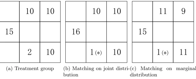
Figure 1: Different control groups selected when the perfect matching cannot be achieved due to the lack of control units in bin (*).
Note that the matching problem is trivial if there exists a control group that perfectly matches the treatment group (i.e., the empirical covariate distributions in the groups are identical). Consider the treatment group in Figure 1a, where the two-dimensional grid (built for two covariates) contains in its cells, termed bins, the number of units found in each bin. If a perfect matching of the control units to the treated ones does not exist, then the selection of a good control group becomes challenging. When a joint distribution is used to capture the dependence between the treatment variable and the covariates, the joint bins can be viewed as being independent and all equally important for representing the distribution. A good matching method should select some control units to form a group with a minimum loss in the joint distribution (Figure 1b). On the other hand, since the joint bins are formed as the intersections of |K| multiple marginal bins, the assumption of the independence between the bins may not be well justified. Then, one can take an alternative approach and select the control group that achieves the best matching in all the marginal distributions (Figure 1c), albeit sacrificing some information captured in the copula. In summary, the problems of matching on the joint or marginal distributions each have their pros and cons, which is why the ensuing computational studies use and compare them both for treatment effect estimation (see Section 5).
3.2 Nonlinear Integer Optimization Problems
The objective of our matching problem is to select such a subsetS ⊆ C that minimizes the MI between the treatment indicator and covariate vector over set S ∪ T. The MI between
t and X (or all theXk) is denoted by I(t;X) if the computation is based on the full joint
distribution of the covariates, and by P
k∈KI(t;Xk) if the computation is based on the
marginal distributions of individual covariates. Since these expressions have similar math-ematical forms, only I(t, X) will be used for notation in the following discussion, with X
representing eitherXorXk, depending on the context. Note thatI(t, X) is an unambiguous
into a one-dimensional range, and hence, can also be treated as a single-covariate problem, albeit possibly with the additional constraints capturing the copula-based dependencies.
In order to express I(t;X) using the empirical covariate distribution for the units in a given problem, denote the covariate value for any unit contained in binbby the same variable
Xb. Letp(t) be the probability that a unit is treated, and p(Xb) be the probability that its
covariate value falls into bin b, with P
b∈Bp(Xb) = 1. Also, let p(Xb, t) be the probability
that the covariate value of a unit with treatment indicator t falls into bin b. Then, the empirical MI between the treatment indicator tand covariateX can be expressed as
I(t;X) =X
b∈B
X
t∈{0,1}
p(Xb, t) log
p(Xb, t)
p(Xb)p(t)
. (1)
Let Sb (or Tb, Cb) denote the number of units in group S (or T, C) with covariate
values falling into bin b. From the characteristics of the units in S ∪ T, the probabilities in equation (1) can be estimated. If t = 0, p(Xb, t) = |S|S+b|T | and p(t) = |S||S|+|T |; if t = 1,
p(Xb, t) =|S|T+b|T | and p(t) = |T |
|S|+|T |; also, p(Xb) = |S|Tb++|T |Sb.
In general, an MI estimation bias (which is different from the causal estimation bias discussed above) arises when the MI estimation is done based on a fixed limited number of observations (1) (Panzeri and Treves, 1996; Roulston, 1999). However, this paper analyzes theempirical distributions of the variables defined for the units in the control and treatment groups, which are available in their entirety, and hence, by (1), the MI is exactly given,
I(t;X) = log (|S|+|T |) + 1
|S|+|T |( X
b∈B
Sb[logSb−log(Tb+Sb)−log|S|]
+X
b∈B
Tb[logTb−log(Tb+Sb)−log|T |]).
(2)
Two alternative MI-based objective functions are analyzed in this paper: I(t;X) and
P
k∈KI(t;Xk). Formally, a problem from the class of Mutual Information based
Matching (MIM) problems is stated:
Given: |K|covariates; treatment groupT; control poolC with|C|>|T |; for each observed unit u ∈ T ∪ C, the covariate vectors X = {X1, X2, ..., X|K|}; segmented covariate space
with joint bins b ∈ B and marginal bins m ∈ M; a fixed integer N as the target control group size.
Objective: find a subsetS ⊆ C such that
• |S|=N and I(t;X) is minimized (MIM-Joint problem), or
• |S|=N and P
k∈KI(t;Xk) is minimized (MIM-Marginal problem).
Theorem 1 The decision version of the MIM-Marginal problem, minS⊂CPk∈KI(t;Xk)
subject to |S|=N, is NP-complete.
Proof See Appendix A.
4. Solution Approaches
This section investigates the properties of solutions with the minimum MI, with the goal of developing a method for treating the nonlinearity in the objective function of MIM problems. The derivations presented in this section unfold from the problem of minimizing I(t;X) under the assumption that the contents of the bins capturing the distribution of covariate
X are independent. The obtained insights are next extended to the Joint and MIM-Marginal problems. The mixed integer programming models and matching algorithms are then developed for selecting control subsets for MIM-Joint and MIM-Marginal problems.
4.1 Analyses of Optimality Conditions
Consider the expression of MI in (2); observe that since the treatment group is given, and the target control group size is known, |S| = N, several terms in equation (2) are constant. Also,P
b∈BSblog|S|+
P
b∈BTblog|T |=|T |log|T |+|S|log|S|. Then, the term
P
b∈BSb[logSb−log(Tb+Sb)] +Pb∈BTb[logTb−log(Tb+Sb)] remains the only one to be
considered for MI minimization. For the ease of presentation, this term can now be rewritten based not on the bins’ aggregate contents but on the individual units’ locations in the bins. Because all the observed units, whose covariate values Xu are contained in the same bin, have the same values ofTb and Sb, the minimization of (2) is equivalent to that of
R≡ Y
u∈S,Xu∈b
Sb
Tb+Sb
Y
u∈T,Xu∈b
Tb
Tb+Sb
. (3)
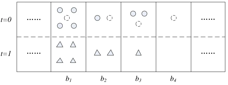
Consider the MIM problem instance illustrated by Figure 2, where N−1 control units have been selected from the control pool into a control group (not necessarily optimally). In order to complete the selection of units into the control group, one last unit has to be selected from any of the bins with Sb < Cb. All such bins can be partitioned into three
subsets: B1 ={b : Sb < Tb}, B2 = {b :Sb ≥ Tb, Tb 6= 0}, B3 = {b :Tb = 0}. Given that
the last unit added to the control group is contained in binb, letIb denote the resulting MI
betweent andX, and Rb denote the resulting objective function value in (3).
The following two lemmas provide the guidelines for the optimal selection of the last unit to be included into the control group.
Lemma 2 Consider an instance where an incomplete control group has N −1 units in it, and three candidate units (that could complete it) are contained in bins b1 ∈ B1, b2 ∈ B2
and b3∈B3, respectively. Then, I1 < I2 < I3.
Proof If the candidate unit from bin b1 ∈ B1 is selected, then the value of Sb1 increases
by 1, while all the other Sb and Tb values stay unchanged. Thus, the objective
func-tion value in (3) becomes R1 = ˆR(
Sb1+1
Tb1+Sb1+1)
Sb1+1( Tb1
Tb1+Sb1+1)
Tb1( Sb2
Tb2+Sb2)
Sb2( Tb2
Tb2+Sb2)
t=0
t=1
……
……
……
……
b
1b
2b
3b
4Figure 2: A selection process illustration. Treated units in T, selected control units in S
and unselected control pool units are represented by triangles, full circles and dashed circles, respectively.
where ˆR represents the terms unrelated to b1 or b2. Similarly, if the candidate unit
from bin b2 ∈ B2 is selected, then the objective function value in (3) becomes R2 =
ˆ
R( Sb1
Tb1+Sb1)
Sb1( Tb1
Tb1+Sb1)
Tb1( Sb2+1
Tb2+Sb2+1)
Sb2+1( Tb2
Tb2+Sb2+1)
Tb2. By the definitions of B1 and B2,
observe that Tb1 ≥Sb1 + 1> Sb1 and Sb2+ 1 > Sb2 ≥Tb2. Therefore,
R1
R2 <1, and hence,
I1 < I2.
If a unit fromb2∈B2orb3 ∈B3is selected to complete the control group, then the
corre-sponding objective function value in (3) is given byR2 = ˆR(
Sb2+1
Tb2+Sb2+1)
Sb2+1( Tb2
Tb2+Sb2+1)
Tb2 or
R3 = ˆR( Sb2
Tb2+Sb2)
Sb2( Tb2
Tb2+Sb2)
Tb2, where ˆRrepresents the terms unrelated tob
2 orb3,
respec-tively. By the definition of B2, observe that Sb2 + 1> Sb2 ≥Tb2, and hence, 0.5<
R2
R3 <1.
Consequently, one has I2 < I3.
Lemma 3 Consider an instance where an incomplete control group has N −1 units in it, and two candidate units (that could complete it) are contained in bins b1, b2 ∈ B1 (or
b1, b2 ∈B2), respectively. Then,I1 < I2 if and only if Sb1−A
Tb1 <
Sb2−A
Tb2 , where A≈ −0.47.
Proof First, consider the case where b1 ∈ B1 and b2 ∈ B1. Similarly to the proof
of Lemma 2, one obtains R1 = ˆR(
Sb1+1
Tb1+Sb1+1)
Sb1+1( Tb1
Tb1+Sb1+1)
Tb1( Sb2
Tb2+Sb2)
Sb2( Tb2
Tb2+Sb2)
Tb2,
and R2 = ˆR( Sb1
Tb1+Sb1)
Sb1( Tb1
Tb1+Sb1)
Tb1( Sb2+1
Tb2+Sb2+1)
Sb2+1( Tb2
Tb2+Sb2+1)
Tb2, and hence, R1
R2 = (1 +
1 Sb1)
Sb1 1
(1+Tb 1
1+Sb1
)Tb1+Sb1
Sb1+1
Tb1+Sb1+1
1
Sb2+1
Tb2+Sb 2+1
1 (1+Sb1
2
)Sb2(1 +
1 Tb2+Sb2)
Tb2+Sb2
= {
(1+ 1
Sb1) Sb1
(1+Tb 1
1+Sb1
)Tb1+Sb1(1+ Tb1
Sb1+1)
}/{
(1+ 1
Sb2) Sb2
(1+Tb 1
2+Sb2
)Tb2+Sb2(1+ Tb2
Sb2+1)
}. Observe that both the
prop-erties of the ratio R1
R2 can be analyzed by studying the properties of function f(x, y) =
(1+x1)x
(1+y+1x)(y+x)(1+ y x+1)
; more specifically, if one can show that f(Sb1, Tb1) < f(Sb2, Tb2), then
one has R1
R2 <1 andI1< I2, and vice versa. Per the properties off(x, y) (see Appendix B),
it is concluded thatf(Sb1, Tb1)< f(Sb2, Tb2) if and only if
Sb1−A
Tb1 <
Sb2−A
Tb2 , whereA
≈ −0.47.
The proof for the case with b1 ∈B2 and b2∈B2 is constructed in the same manner.
Given the arbitrary bins b1 ∈ B1, b2 ∈ B2 and b3 ∈ B3, I1 < I2 < I3, by Lemma 2
and by the definition of the subsets B1, B2 and B3, one has Sb1−A
Tb1 < 1,
Sb2−A
Tb2 >1, and
Sb3−A
Tb3 = +∞. Therefore, Lemma 2 can be viewed as a special case of Lemma 3. Having considered the problem of optimally adding a single unit to the existing (incomplete) control group, the obtained results are now generalized to the problem of selecting a whole control group of a given size.
Theorem 4 (Necessary and Sufficient Condition for Optimality) Consider an instance of minimizing I(t;X). A control group S of size N is optimal if and only if for any pair of bins b1 and b2 with |Cb2 −Sb2| ≥1 it holds that
Sb1−1−A
Tb1
≤ Sb2 −A
Tb2
, (4)
where A≈ −0.47.
ProofThe proof will proceed by contradiction. For convenience, in the following narrative, any group violating the theorem’s condition is termed animprovable group. For an improv-able group, one can identify at least one pair of bins, b1 and b2, such that |Cb2 −Sb2| ≥1
and Sb1−1−A
Tb1 >
Sb2−A
Tb2 . Any such pair is termed animprovable pair.
First, consider the necessary condition for optimality: if a group is optimal, then it is not an improvable group. Suppose that S is an optimal group with the minimumI(t;X), andS is also an improvable group. Without loss of generality, assume thatb1 andb2 are an
improvable pair and Sb1−1−A
Tb1 >
Sb2−A
Tb2 . Consider an incomplete control group of sizeN−1, obtained by removing a control unit from bin b1 in S. Because
(Sb1−1)−A
Tb1 >
Sb2−A
Tb2 and according to Lemma 3, one can obtain a group with a smaller value of I(t;X) by adding the last unit into binb2. Thus, S is not optimal, and one arrives at a contradiction.
Second, consider the sufficient condition for optimality: if a group is not an improvable group, then it is optimal. Suppose that S is not an improvable group, S∗ is an optimal group with the minimum I(t;X), and S∗ 6=S. Then, there must exist some bin(s) where
S∗ has fewer units thanS, and some other bin(s) whereS∗has more units thanS. Without
loss of generality, assume thatb1 andb2 are two such bins, respectively. SinceS∗ has more
units in binb2 thanS, this implies|Cb2 −Sb2| ≥1. BecauseS is not an improvable group,
one has Sb1−1−A
Tb1
≤ Sb2−A
Tb2 .
If Sb1−1−A
Tb1 <
Sb2−A
Tb2 , then according to Lemma 3, if a unit is removed from b1 and
I(t;X), with Sb1−1−∆−A
Tb1 <
Sb1−1−A
Tb1 <
Sb2−A
Tb2 <
Sb2+∆−A
Tb2 holding for ∀∆>0. Note again that b1 and b2 were arbitrarily picked. Such unit shuffling (i.e., removal and addition)
operations can repeat until S is modified to become identical toS∗. Since in this process,
I(t;X) increases with every shuffle, thenS∗ could not be optimal, which is a contradiction. If Sb1−1−A
Tb1 =
Sb2−A
Tb2 , then as a result of removing a unit fromb1 and adding one intob2,
I(t;X) will not change. In such a case, if the updatedS becomes identical to S∗, then this means thatS is an alternative optimal solution with the minimum I(t;X). Otherwise, one can continue shuffling units, with Sb1−1−∆−A
Tb1 <
Sb1−1−A
Tb1 =
Sb2−A
Tb2 <
Sb2+∆−A
Tb2 holding for
∀∆>0. Similarly,I(t;X) will continue increasing, leading toS∗ not being optimal, i.e., to a contradiction.
Theorem 4 provides the necessary and sufficient optimality conditions for the control groups with the minimum I(t;X). Its value lies in condition (4) being linear in Sb, unlike
the minimization problem objective (2). Note, however, that Theorem 4 only works to determine whether a control group is optimal or not; it cannot be used to assess or compare the quality of suboptimal control groups.
In order to effectively apply Theorem 4 in practice, one would like to avoid the exhaustive traversal of bin pairs. Corollaries 5 and 6 allow for tackling this problem and provide a means for efficient optimal control group selection.
Corollary 5 Consider an instance of minimizingI(t;X)whereN >P
b∈{b:Tb≥1}Cb. Then, a control group S is optimal if it includes all the control units in all b∈ {b:Tb ≥1}.
Proof Follows directly from Lemma 2.
Corollary 6 Consider an instance of minimizing I(t;X), where N ≤ P
b∈{b:Tb≥1}Cb. Then, a control group S is optimal if and only if for every pair of bins b1 and b2 such
that
b1 ∈argmax b∈B
{Sb−1−A Tb
} (5)
and
b2 ∈argmin b∈B
{Sb−A Tb
:|Cb−Sb| ≥1}, (6)
one has Sb1−1−A
Tb1
≤ Sb2−A
Tb2 , where A
≈ −0.47.
ProofConsider any pair of bins,b3 and b4, with|Cb4−Sb4| ≥1. In order to determine ifS
is optimal, Theorem 4 prescribes to compare the left-hand and right-hand sides of inequality (4) for binsb3 and b4. By the statement of this corollary, one has
Sb1−1−A
Tb1 ≥
Sb3−1−A
Tb3 and
Sb2−A
Tb2 ≤
Sb4−A
Tb4 . Then, if inequality (4) holds for bins b1 andb2, then it also holds for bins
B3 and B4, because
Sb3−1−A
Tb3 ≤
Sb1−1−A
Tb1 ≤
Sb2−A
Tb2 ≤
Sb4−A
4.2 Mixed Integer Programming-Based Matching Algorithms
The optimality conditions in Theorem 4 and Corollary 6 allow one to construct an alter-native formulation for the problem of minimizing I(t;X) with N ≤P
b∈{b:Tb≥1}Cb, using the expression Sb−1−A
Tb . Note that this ratio is undefined for bins with Tb = 0; however, per Lemma 2, an optimal solution can contain control units from such bins only if all the available control units from other bins have been exhausted. In order to reformulate the ob-jective function of minimizingI(t;X), the expression Sb−1−A
Tb should first be revised so that its denominator evaluates to a fixed number,α∈(0,1), small enough to make the selection of control units from bins with Tb = 0 very costly. In order to search for a control group
satisfying the condition in Corollary 6, the following optimization problem is formulated:
min
S⊂C{maxb∈B
Sb−1−A
max{Tb, α}}, (7)
where α is a positive parameter small enough to distinguish Tb = 0 from other positive
values ofTb, e.g., α= 0.01.
By solving (7), one can work to construct an optimal control group through minimizing the maximum value of the function in (5). Having found an optimal solution to (7), one can check if (for this solution) the set in (5) is a singleton. If it is, then the condition in Corollary 6 holds. Otherwise, satisfying (7) may not be sufficient for satisfying Corollary 6, since it requires one to check every pair of bins in both the set in (5) and the set in (6). As an example of this situation, suppose that there exist two bins, b1 and b3, in the set
in (5), and a bin b2 in the set in (6) such that
Sb1−1−A
Tb1 =
Sb3−1−A
Tb3 >
Sb2−A
Tb2 . If a unit is removed from b1 while another unit is added into b2, the objective value of (7) does not
improve because Sb3−1−A
Tb3 does not decrease. Thus, the optimization process based purely on solving (7) would terminate early without guaranteeing an optimal matching.
To handle the situation where the set in (5) is not a singleton for a solution of (7), an algorithm is developed to iteratively solve for the optimal number of units to be selected from each bin. In any iteration, if solving (7) returns multiple bins with values of Sb−1−A
Tb equal to the maximum (over all the bins), then one of these bins is added to a “forbidden bin set”, denoted by BF and initialized at an empty set before the first iteration. Every timeBF is updated, problem (7) is reformulated, with all the bins that are not inBF, and solved again in the next iteration. After several such iterations, once the set in (5) is found to be a singleton for a solution to (7), one can be sure that an optimal control group has been found. In order to ensure that the unit picking in a given iteration does not mess up the optimality achieved within any bin in the previous iteration(s), a bin with the smallest number of the treatment units in the non-singleton set (5) is always fixed first. In every iteration, (7) is solved as a mixed integer programming (MIP) model,
min q (8)
s.t. q≥ Sb−1−A
max{Tb, α}
∀b /∈BF, (9)
X
b∈B
Sb≤Cb ∀b∈B, (11)
Sb≥0 ∀b∈B, (12)
Sb :integer ∀b∈B, (13)
B ={b:Cb+Tb ≥1}. (14)
The decision variables in this MIP are the numbers of the control units,Sb, to be selected
from each bin. Since it is only necessary to consider the bins in {b : Cb+Tb ≥ 1}, then
despite the fact that the total number of joint bins grows exponentially with the binning partition granularity, the number of the decision variables is bounded by |T |+|C|. The contents of the forbidden bin set BF are updated iteratively in the described algorithm. The minimax optimization problem (7) is formulated with the objective function (8) and the constraint set (9). Constraint (10) ensures that the total number of units in the control group is equal toN. Constraints (11), (12) and (13) restrict the range ofSb to nonnegative
integers not exceeding the number of available control units in each respective bin.
Note that for solving any MIM-Joint problem, since the bins’ contents can be treated as being independent from each other, the described procedure for minimizing I(t;X) can be exactly followed to minimize I(t;X), with binsb in (8)-(14) being the joint bins.
Algorithm 1 MIP-based matching for MIM-Joint problem
1: Initialize the bin set{b:Cb+Tb ≥1} consisting of all the bins occupied by the units
inT ∪ C; computeTb and Cb; forbidden bin setBF =∅.
2: Update and solve the corresponding instantiation of formulation (8)-(14) to obtain Sb
for every binb.
3: If argmaxb /∈BF{Sb−T1−A
b } is a singleton, go to step 4. Otherwise, add the bin with the smallest number of treatment units in argmaxb /∈BF{Sb−T1−A
b } into set B
F, record and
fix the optimal number of control units to be selected in it, and go to step 2.
4: Construct a control group complying with the obtained values ofSb over all the
initial-ized binsb. Stop.
However, for solving an MIM-Marginal problem, modifications to the above formulation and the algorithm are necessary due to the fact that the marginal bins cannot be assumed independent. The decision variables of an MIP-Marginal model are the numbers of control units to be selected into S for every joint bin (b still denotes a joint bin), and constraints (10)-(14) remain a part of the optimization problem. Let m denote a marginal bin, MF
denote the forbidden marginal bin set, and Tm, Cm and Sm denote the number of all the
treatment units, number of all the control units and number of the selected control units in
m, respectively. Equation (9) is then replaced by (15). Also, an additional constraint (16) is added to the formulation to ensure that the number of units in any marginal bin equals the summed total number of units in all the corresponding joint bins.
q≥ Sm−1−A
max{Tm, α}
∀m /∈MF, (15)
Sm=
X
b;Xm∈b
Recall that in every iteration of solving MIM-Joint using Algorithm 1, one checks whether the set of bins with the maximum value of Sm−1−A
Tm is a singleton. Because of the dependence between the contents of marginal bins, this condition by itself does not guarantees optimality for MIM-Marginal problem. Specifically, given a feasible solution to an MIM-Marginal problem, if exactly one marginal bin is found to achieve the maximum value of Sm−1−A
Tm and this marginal bin is associated with covariatek, then because the bins in the same covariate are independent and according to Corollary 6,I(t;Xk) is minimized.
But the MI in other covariates might still be improved without changing I(t;Xk), e.g., by
adding and removing the same number of control units to/from the same marginal bin in covariatek. Thus, while solving for the optimal number of units in each marginal bin, and adding the marginal bins one-by-one to a forbidden bin set, one should not stop until the sets of bins with the maximum values of Sm−1−A
Tm in all the|K|covariates become singletons.
Algorithm 2 MIP-based matching for MIM-Marginal problem
1: Initialize the joint bin set{b:Cb+Tb≥1}and the marginal bin set{m:Cm+Tm≥1}
consisting of all the bins occupied by the units inT ∪ C; computeTb,Cb, Tm and Cm;
forbidden bin set MF =∅.
2: Update and solve the corresponding instantiation of formulation (8), (10)-(16) to obtain
Sb for every joint bin b.
3: If argmaxm /∈MF{Sm−T1−A
m }is a singleton for every covariate, go to step 4. Otherwise, add the marginal bin with the smallest number of treatment units in argmaxm /∈MF{Sm−T1−A
m }
into set MF, record and fix the optimal number of control units to be selected in it, and go to step 2.
4: Construct a control group complying with the obtained values ofSb over all the
initial-ized binsb. Stop.
4.3 Sequential Selection Matching Algorithms
Based on the optimality conditions in Theorem 4, Algorithms 1 and 2 are guaranteed to achieve best matched control groups for MIM-fixed and MIM-marginal problem instances. However, their MIPs may become difficult to solve for problems of large size, which, however, can be avoided by utilizing the result captured in Theorem 7, presented for the problem of minimizing I(t;X).
Theorem 7 If control group S has the minimum I(t;X) among all the control groups of size N, then a group with the minimum I(t;X) among all the control groups of size N+ 1 (N−1) can be obtained fromS by adding to it a single unit from binb∈argminb∈B{
Sb−A
Tb :
|Cb−Sb| ≥1} (removing from it a single unit from bin b∈argmaxb∈B{Sb
−1−A
Tb }).
Proof LetS+ denote a control group obtained from S by adding to it a single unit from
bin b∈argminb∈B{Sb−A
Tb :|Cb−Sb| ≥1}. According to Lemma 3, the MI between T and
X over set T ∪ S+ is minimal among all the groups that can be built onS. The following
Let Sb+ denote the number of control units selected into S+ in bin b. Let b 1 and
b2 be two bins such that b1 ∈ argmaxb∈B{
Sb+−1−A
Tb } and |Cb2 −S
+
b2| ≥ 1. If b1 is the
bin where S+ has one more unit than S, then S+
b1 −1 = Sb1 and S
+
b2 = Sb2, and then
S+b
1−1−A
Tb1 =
Sb1−A
Tb1 ≤
Sb2−A
Tb2 =
Sb+
2−A
Tb2 . Note that by Theorem 4, because S is optimal, one has Sb1−1−A
Tb1 ≤
Sb2−A
Tb2 . Ifb2 is the bin whereS
+has one more unit thanS, thenS+
b2−1 =Sb2
and S+b
1 =Sb1, and then
Sb+
1−1−A
Tb1 =
Sb1−1−A
Tb1 ≤
Sb2−A
Tb2 <
S+b
2−A
Tb2 . IfS andS
+ have the same
numbers of units in both b1 and b2, then Sb+
1−1−A
Tb1 =
Sb1−1−A
Tb1 ≤
Sb2−A
Tb2 =
Sb+
2−A
Tb2 . Therefore, by Corollary 6, S+ is a group with the minimum I(t;X) among all the control groups of
sizeN + 1.
Let S− denote a control group obtained from S by removing a single unit from bin
b ∈ argmaxb∈B{Sb
−1−A
Tb }. Let S
−
b denote the number of control units selected into S
− in
bin b. Letb1 and b2 be two bins such that b1 ∈argmaxb∈B{
S−b−1−A
Tb } and |Cb2 −S
−
b2| ≥1.
If b2 is the bin where S has one more unit than S−, then Sb2 −1 = S
−
b2 and S
+
b1 = Sb1,
and then S
−
b1−1−A
Tb1 =
Sb1−1−A
Tb1 ≤
Sb2−1−A
Tb2 =
S−b
2−A
Tb2 . Note that due to the optimality of S,
Sb1−1−A
Tb1 ≤
Sb2−A
Tb2 . Ifb1 is the bin where S has one more unit thanS
−, thenS
b1 −1 =S
−
b1
and S+b
2 =Sb2, and then
Sb−
1−1−A
Tb1 <
Sb1−1−A
Tb1 ≤
Sb2−A
Tb2 =
S−b
2−A
Tb2 . IfS andS
+ have the same
numbers of units in both b1 and b2, then Sb−
1−1−A
Tb1 =
Sb1−1−A
Tb1 ≤
Sb2−A
Tb2 =
Sb−
2−A
Tb2 . Therefore, by Corollary 6, S− is a group with the minimum I(t;X) among all the control groups of sizeN −1.
Theorem 7 provides a method for finding optimal control groups for MIM problems, without solving any programming models. One can iteratively build control groups of increasing sizes until an optimal solution of the desired size N is obtained. Each control group in this process results in the minimum value of MI among all the groups of the same size. Also, Theorem 7 provides establishes a relationship between the optimal subsets for problems with different target control group sizes. This result will be important for seeking the minimum MI in the problems with an unrestricted (flexible) control group size.
For the MIM-Joint problem, since its bins are treated as independent from each other, Theorem 7 directly applies, and Algorithm 3 guarantees to return an optimal solution. Note that Algorithm 3 is polynomial. In the worst case, it needs to make comparisons of Sb−A
Tb forN multiples of the number of bins occupied by treatment units.
With the MIM-Marginal problem, a challenge arises due to the dependence between the marginal bins’ contents. By comparing the terms Sm−A
Tm , one can identify the marginal bin to which a control unit should be added, but one still needs to pick some joint bin. Even further, since the marginal bins on the same covariate are independent from each other, the comparison of Sm−A
Algorithm 3 Sequential selection matching for MIM-Joint problem
1: Initialize the joint bin set {b :Cb +Tb ≥1} consisting of all the bins occupied by the
units inT ∪ C; computeTb and Cb; set Sb= 0 for all b.
2: Select a binb∈argminb∈B{Sb−A
Tb :|Cb−Sb| ≥1}, updateSb by adding 1. 3: IfN units are selected, go to step 4. Otherwise, go to step 2.
4: Construct a control group complying with the obtained values ofSb over all the
initial-ized binsb. Stop.
to achieve good (but not necessarily optimal) solutions to MIM-Marginal instances in the following manner. For each joint unit,|K|ratios of the form Sm−A
Tm are evaluated (one per covariate); these |K| ratios are organized in a descending order; then, the joint bin with the lexicographically minimal ratio gets one more unit added to it. Again, the resulting Algorithm 4 is an approximate method, but it is polynomial, and in practice, is found to return solutions of high quality for diverse matching problem instances (see Section 5).
Algorithm 4 Sequential selection matching for MIM-Marginal problem
1: Initialize the joint bin set {b :Cb +Tb ≥1} consisting of all the bins occupied by the
units inT ∪ C; computeTb and Cb; set Sb= 0 for all b.
2: Update Sm−A
Tm for each marginal bin, and order all associated
Sm−A
Tm by values in descend sequence for each joint bin.
3: Find a binbin set{b:|Cb−Sb| ≥1}such that its ordered set ofSm−A
Tm is lexicographically minimal; increase the value of the decision variable,Sb, corresponding to this bin, by 1.
4: IfN units are selected, go to step 5. Otherwise, go to step 2.
5: Construct a control group complying with the obtained values ofSb over all the
initial-ized binsb. Stop.
The complexity of Algorithm 4 depends on the number of covariates |K|, the number of marginal bins |M|, treatment group size|T |, control pool size |C|and target control group sizeN. In the worst case, every unit (treated or control) occupies one unique joint bin, with each joint bin contributing to|K|marginal bins. The storage of these data requires a space of size O(|K|(|T |+|C|)). In the binning step, both the treatment group and control pool are traversed, with each unit being assigned to the appropriate marginal and joint bins: this operation takes O(|M|(|T |+|C|)) time. In the matching step, all the occupied joint bins are traversed for the lexicographic comparison, which takesO(N(|T |+|C|)|K|2) time.
5. Computational Analyses
5.1 Algorithm Performance Assessment
In order to evaluate the performance of the MIM algorithms, a series of tests is first con-ducted with the data set designed by Sauppe et al. (2014), which was found challenging for the existing matching methods1. This synthetic data set with 25 covariates contains 100 treatment units and 10,000 control units. All the covariate values are drawn from nor-mal distributions with mean 0. All the treatment and control units have the same, highly nonlinear response function. Thus, by design, the average treatment effect for the treated (ATT) for the created population is zero.
The experiments were conducted with the number of the considered covariates varied in the range from 1 to 25. In optimizing the covariate balance, Sauppe et al. (2014) uniformly partitioned the range of the observed unit values in each covariate into 20 bins, and used Balance Optimization Subset Selection (BOSS) for control group selection. In order to treat the instances resulting in large MIP formulations, Sauppe et al. (2014) adopted a time limit heuristic. They achieved quite well balanced control groups; however, the limited computa-tional efficiency remains the key challenge for the existing BOSS methods, especially when the data sets to make inference from are very large.
With the same settings as in Sauppe et al. (2014), this section compares the performance of the following matching methods: the Mahalanobis distance-based one, the propensity score-based one, the BOSS methods from Sauppe et al. (2014), and three MIM methods – MIM-Joint, MIM-Marginal MIP, and MIM-Marginal sequential selection. Note that the first two of these methods are widely used and included in several existing matching packages, e.g., MatchIt (Ho et al., 2011) and optmatch (Hansen and Klopfer, 2012). We also used Coarsened Exact Matching (CEM) in MatchIt (Ho et al., 2011) and fullmatch method in optmatch (Hansen and Klopfer, 2012). However, CEM excluded many treatment units from the matched treatment group in the experiments with five or more covariates, and thus, was not found suitable for ATT estimation. Also, under the pre-set control group size, the results of fullmatch were no different from those of the standard Mahalanobis distance or propensity score matching (depending on the selected parameter settings).
The MIP models for MIM were solved using CPLEX. To reduce the runtime in solving some large-size problems, a heuristic was applied that utilized the solution of sequential selection to covert MIP to an integer program. Generally, MIP-based methods (be it for BOSS or MIM) are time-consuming. However, the sequential selection algorithm always runs very quickly: it took about 7 seconds on average to find solutions for the instances with 25 covariates on a desktop with an Intel Xeon E5-2420 1.9GHz CPU and 16G RAM.
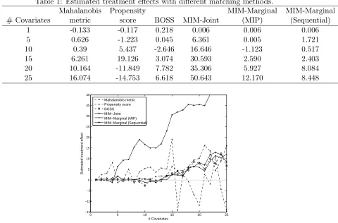
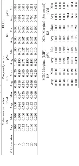
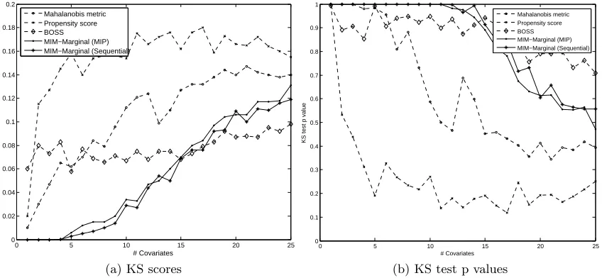
Table 1 presents the ATT estimates obtained with the considered methods for the in-stances with the varied number of covariates; Figure 3 provides a graphical illustration of the results. Recall that by design, the ATT is zero, so the closer an estimate is to zero, the better. Table 2, Figure 4a and Figure 4b report the Kolmogorov-Smirnov (KS) test statistic scores and associated p-values for checking whether the underlying covariate distributions differ in the treated and control groups. In Table 2, column “Avg” reports the average
1. The data set, named 25c10k, features a highly nonlinear response function and is available in full in the online supplement of Sauppe et al. (2014). The response function in it isy= 0.8x1(1.0−x1)+0.5x2(0.7+
x1) + 0.27x3x2−0.9x24+ 0.7x5(0.5 +x5)x2−0.6x6x1+ 0.4x7−0.8x8+ 0.6x9(0.9−x9) + 0.2x210(0.3−x7) +
0.5x211−1.4x12−0.8x13−0.9x214+ 0.5x215(0.1 +x15) + 0.8x16−0.9x17(0.2−x13) + 1.5x18−1.2x19(1.0 +
Table 1: Estimated treatment effects with different matching methods.
Mahalanobis Propensity MIM-Marginal MIM-Marginal
# Covariates metric score BOSS MIM-Joint (MIP) (Sequential)
1 -0.133 -0.117 0.218 0.006 0.006 0.006
5 0.626 -1.223 0.045 6.361 0.005 1.721
10 0.39 5.437 -2.646 16.646 -1.123 0.517
15 6.261 19.126 3.074 30.593 2.590 2.403
20 10.164 -11.849 7.782 35.306 5.927 8.084
25 16.074 -14.753 6.618 50.643 12.170 8.448
0 5 10 15 20 25
−15 −10 −5 0 5 10 15 20 25 30 35 40
# Covariates
Estimated treatment effect
Mahalanobis metric Propensity score BOSS MIM−Joint MIM−Marginal (MIP) MIM−Marginal (Sequential)
Figure 3: Trends for estimated treatment effects with different matching methods.
KS distance or p-value over all the covariates, and columns “Max” and “Min” report the maximum KS test statistic and minimum p-values, respectively. The smaller the KS score and the larger the p-value, the better balance is achieved.
In general, the MIM-Joint does not output accurate treatment effect estimates in the multi-covariate cases. If an exact or almost-exact matching solution exists, the MIM-joint performs well, e.g., as in the one-covariate case. However, it is too sensitive to imbalance. As the number of the covariates grows, there remain fewer and fewer bins in which exact matching is possible, making the MIM-Joint formulation not-so-useful for most practical cases. At the same time, the marginal bin-based matching methods succeed in obtaining rather accurate ATT estimates.
0 5 10 15 20 25 0
0.02 0.04 0.06 0.08 0.1 0.12 0.14 0.16 0.18 0.2
# Covariates
KS score
Mahalanobis metric Propensity score BOSS MIM−Marginal (MIP) MIM−Marginal (Sequential)
(a) KS scores
0 5 10 15 20 25
0 0.1 0.2 0.3 0.4 0.5 0.6 0.7 0.8 0.9 1
# Covariates
KS test p value
Mahalanobis metric Propensity score BOSS MIM−Marginal (MIP) MIM−Marginal (Sequential)
(b) KS test p values
Figure 4: Trends for marginal balance quality for matching solutions.
instances with more than 15 covariates, the large number of bins makes for a large variance in the ATT estimates; comparing only the 100 treatment units and the 100 matched control units, one observes significant divergence between the ATT and its estimates obtained with all the methods, even though BOSS achieves the smallest KS scores. Considering both the matching quality and runtime performance, the MIM-Marginal with sequential selection algorithm comes out as the most efficient matching method for practical purposes.
5.2 The Experiences with Using Mutual Information as a Measure of Balance
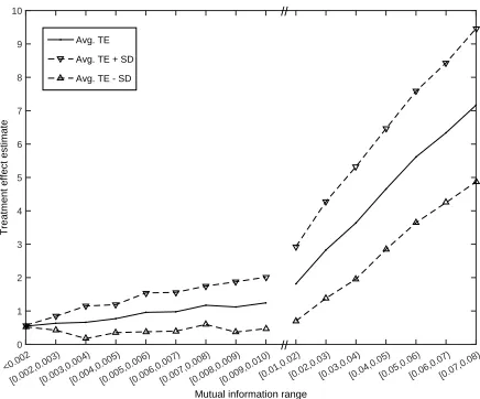
The next set of experiments reveals that the MI function, employed as the objective in MIM, can be viewed as a surrogate measure of covariate balance. In order to trace the dependence between the MI values, obtained with different control groups, and the corresponding ATT estimates, an additional set of results is reported with the data set of Section 5.1 with 10 covariates. This set is also used to help us assess the impact of the MIM algorithm parameter settings on the matching quality
For a large number of randomly generated control groups, the MI values were recorded together with the resulting treatment effect estimates (see Figure 5). Among these, four groups were found to have the MI less than 0.002 and at least 100 groups fell in each of the other intervals, into which the MI range was divided. Observe that, as the MI grows, the average of the ATT estimates tends to increase, and the standard deviation of the estimate values over the intervals grows as well. This confirms the premise that minimizing MI is a valid approach to guiding the matching process.
Mutual information range
<0.002
[0.002,0.003)[0.003,0.004)[0.004,0.005)[0.005,0.006)[0.006,0.007)[0.007,0.008)[0.008,0.009)[0.009,0.010)[0.01,0.02)[0.02,0.03)[0.03,0.04)[0.04,0.05)[0.05,0.06)[0.06,0.07)[0.07,0.08)
Treatment effect estimate
0 1 2 3 4 5 6 7 8 9 10
// //
Avg. TE Avg. TE + SD Avg. TE - SD
Figure 5: Trends for estimated treatment effects with different mutual information ranges.
20 40 60 80 100 120 140 160 180 200 0
0.5 1 1.5 2 2.5 3 3.5
Control group size
Absolute value of treatment effect estimate
20 40 60 80 100 120 140 160 180 2000 0.002 0.004 0.006 0.008 0.01 0.012 0.014
Mutual information
Mutual Information Treatment effect
Figure 6: Trends for estimated treatment effects with different control group sizes.
the control groups of different sizes can be compared on the same scale, and hence, the optimization of the control group size becomes possible.
5.3 Experiences with Large Data Sets
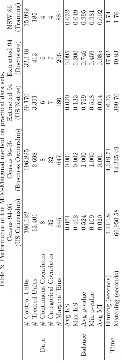
In order to test the performance of the presented MIM methods with large data sets, three suitable real-world data sets were identified. The first one contains weighted census data extracted from the 1994 and 1995 Current Population Surveys conducted by the U.S. Census Bureau (Lichman, 2013): it contains 199,523 records with 41 demographic and employment related variables. The second one was extracted from the 1994 Census database (Lichman, 2013): it contains 32,561 records with 14 variables. The third one was collected in a study focusing on the National Supported Work Demonstration Program (NSW) (LaLonde, 1986), where the randomized job training experiment benchmark was obtained for the treatment effect: it contains 16,177 records with 8 variables. Of the three data sets, only the third one was originally created for a matching purpose. The aim of its creator was to examine how well the statistical methods would perform in trying to replicate the result of a randomized experiment (LaLonde, 1986). To design the test instances with the different number of covariates and varied control pool and treatment group sizes, the first data set was split into a treatment group and a control pool by “US citizenship” and “Business ownership” indicators, respectively; and the second data set was split by “US native” and “Doctorate degree” indicators, respectively. To apply the MIM-Marginal method, each continuous covariate’s range was partitioned into 20 bins, while all the categorical covariates kept their original categories. The target control group size was set equal to the treatment group size. Table 3 gives an aggregate view of the data sets’ specifics, and MIM results and runtimes.
Overall, the MIM-marginal method achieves very good balance across all the covariates. The average KS scores in all the tests are below 0.01 and the averagep-values are all greater than 0.05. Note that since the treated and control data sets in every test are distinct, the results cannot be meaningfully compared across the test instances. For example, the best balance metric values were achieved in the experiment the “Business ownership” data set, even though it had more units and covariates than some other data sets. In the experiment with the “US citizenship” data set, the matching algorithm performed the worst. Indeed, this was a challenging test instance with the target control group size of 13,401, amounting to about 7.2% of the control pool: in such a case, the method is forced to pick non-optimal units to reach the target size, and hence, increases the imbalance. Note, however, that selecting such a large size control group might not be a good idea in practice anyway.
Excellent computational efficiency of the MIM-Marginal method is unparalleled by any other matching method, making it highly practical for data mining; its runtime requirement grows polynomially with the problem size. For example, the “US citizenship” test instance features a very large data set: compared to the training data set, it has 11.6 times more control units, 72.4 times more treated units, significantly larger target control group size, and 5 times more covariates. Yet, the MIM-Marginal runtime with the the “US citizenship” is only 38,040 times larger.
The runs of MIM-Marginal with the NSW data set produce a solution set with mean 1,851.5 and standard deviation 92.1. The average MI over this set is 0.002383; see the achieved balance metrics in Table 3. Importantly, if one removes the target control group size restriction and allows the MIM-Marginal to optimize over it, then a solution with 169 control units is obtained, with the MI of 0.001824 and ATT estimate set with mean 1,818.2 and standard deviation 91.2.
6. MIM Limitations and Future Research Directions
While the presented computational investigations demonstrate the utility of the MIM methodology, this work has its limitations and desirable directions for further improvement. First, this paper does not offer an approach to the calculated selection of a binning scheme. The discretization of the covariate space affects the MI-based estimation outputs, however, the present MIM algorithms take the binning scheme as an input and do not work to perturb it to account for the differences in the shapes of the distributions of different covariates or the distances between bins. Intuitively, if the binning is coarse then the MIM cannot be expected to produce high quality solutions. While binning has been a point of research in multiple branches of optimization-based matching literature, the design of binning structures is still an open question. Another point, relevant to the MI based methods specifically, is that mutual information could be employed in its continuous form, in which case the accuracy of matching might be improved without the use of bins.
Second, in its current form as a non-parametric matching methodology, MIM does not differentiate the covariates by relative importance. Moreover, if there is any indispens-able information of the form of the response function, covariate relationships, or covariate distributions that is not captured via binning, MIM may underperform. There may even exist circumstances where MIM would be consistently unsuccessful in producing accurate treatment effect estimates: such circumstances, as those exposed by Sauppe et al. (2014) with propensity score-based matching, are yet to be explored with MIM. In any case, prior to using MIM, the researcher must be careful about selecting the covariates to work with. Indeed, data preprocessing has been a topic of research worth much attention. Distance-based matching methods employ weights to emphasize the importance of balancing certain some covariates over others. The developments in propensity score-based methods led to the introduction of the concept of “fine balance”. Expanding the MIM research in a similar direction would add to its value.
Finally, by relaxing the integrality constraints of the MIM problems’ decision variables, one could produce linear (non necessarily integer) solutions allowing for insightful interpre-tations. The research in this direction might remedy the MIM dependence on binning.
7. Conclusion
for matching on a single covariate and on the joint distribution of multiple covariates, allowing one to remove non-linear terms from the original mutual information formula and leading to a mixed integer programming formulation of the problem. A sequential selection algorithm is presented that runs in polynomial time and obtains optimal solutions for the problems of matching on a single covariate and matching on a joint distribution of multiple covariates.
Appendix A. Proof of Theorem 1
The decision version of the matching problem on marginal covariate distributions with a fixed target control group size (MIM-Marginal) can be stated as follows. Given a treatment group T, a control pool C and a set of covariates Xk, k ∈ K. Let m be a marginal bin.
(In this proof, it is not necessary to indicate which covariate this marginal bin partitions.) Given parametersγ andN, do there exist subsetsS ⊂ Csuch thatP
k∈KI(T;Xk)≤γ and
|S|=N?
First, it has to be proven that MIM-Marginal belongs to the NP class. For any given subset, one can check that the subset contains exactly N units, and then, calculate the mutual information value as in 2 to check if it is smaller or equal to γ. This can be completed in polynomial time, thus MIM-Marginal belongs to NP.
Second, it has to be proven that MIM-Marginal is NP-hard. Letδumbe a binary variable,
with δum = 1 if unit u belongs to m, and 0 otherwise; let ηu be another binary variable,
with ηu = 1 if unit u is selected into S, and 0 otherwise. Let Tm denote the number of
units in groupT with the values of covariates falling into binm. If letγ = 0 and N =|T |, then problem’s objective is to check whether a perfect matching exists, i.e., whether the following constraints can be simultaneously satisfied:
|C| X
u=1
δumηu =Tm ∀m, (17)
|C| X
u=1
ηu =N, (18)
ηu ∈ {0,1} ∀u,
whereηuis the decision variable. Constraint (17) ensures that a perfect matching is achieved
in each covariate. Constraint (18) limits the size of a control group that can be selected. Note that, sinceN =|T |and each unit belongs to exactly|K|marginal bins, then converting the constraints (17) and (18) into inequalities does not affect the optimal set of the problem, which can now be stated as
|C| X
u=1
δumηu ≥Tm ∀m,
|C| X
u=1
ηu ≤N,
ηu ∈ {0,1} ∀u.
Let δ0ij be a binary variable, with δij0 = 1 if element j is included in set Ii ∈ I, and 0
otherwise; letη0ibe another binary variable, withηi0 = 1 if setIiis selected, and 0 otherwise.
The objective of the SC problem is to findη0 such that
|I| X
i=1
δij0 ηi0 ≥1 ∀j ∈J,
|I| X
i=1
η0i≤n,
ηi0 ∈ {0,1} ∀i.
Define the following mapping: Tm = 1, N =n, u = i, m = j, δum =δij0 and ηu =ηi0.
Thus, the SC problem has a feasible solution if and only if the corresponding MIM-Marginal has a solution. The transformation required to execute the described mapping can be completed in polynomial time in the size of problem inputs. This completes the proof.
Appendix B. Properties of the Ratio Function f(x, y) in Lemma 3
This Appendix analyzes how the values of function f(x, y) = (1+
1
x) x
(1+x+1y)(x+y)(1+ y x+1)
can be
compared for arbitrary inputs (x, y), with x >0 andy >0.
Define functiong(x, y)≡logf(x, y) =xlog(1 +1x)−(x+y) log(1 +x+1y)−log(1 +1+yx) =x(log(1 +x)−log(x))−(x+y)(log(1 +x+y)−log(x+y))−(log(1 +x+y)−log(1 +x)) = (1 +x) log (1 +x)−xlog(x)−(1 +x+y) log(1 +x+y) + (x+y) log(x+y).
Then, ∂g∂x = log(1+x)−log(x)+log(x+y)−log(1+x+y) and ∂g∂y = log(x+y)−log(1+x+y).
Also, ∂x∂g = f1∂f∂x and ∂g∂y = f1∂f∂y.
Because x > 0 and y > 0, one has 1 +x+y > 1 +x > 0. Also, the logarithm is a monotonically increasing function with the monotonically decreasing slope, and hence, one has log(1 +x)−log(x) >log(1 +x+y)−log(x+y)> 0, which implies that ∂g∂x >0 and
∂g
∂y <0. Moreover, sincef >0, then ∂f
∂x >0 and ∂f ∂y <0.
To sum up, the function of interest is monotonic along both x and y directions. This prompts one to study its contour lines over the feasible range of inputs (x, y) (Figure 7). Unfortunately, even though the contours look linear, it does not seem possible to produce a closed-form expression for them, of the formf(x, y) =C, with constantC.
Sincef(x, y) =Cis approximately a straight line for every specificC, then the values of
f(x, y) under different inputs can be compared by evaluating the slopes of the corresponding
contour lines: dydx =−
∂f ∂x ∂f ∂y
=−
∂g ∂x ∂g ∂y
= log(1+log(1+x+xy))−−log(log(xx)+y) −1. Let h(x, y)≡ dydx. For arbitrary (x0, y0) and (x1, y1) such that f(x0, y0) =f(x1, y1), one has h(x0, y0) =h(x1, y1) = xy11−−yx00;
thus, one can study the linearizationh(x, y) off(x, y). Since these contour lines are straight and do not intersect in the first quadrant, they must have a unique, common intersection point. Thus, one can write h(x, y) = y−A2
x−A1, where (A1, A2) are the coordinates of that
unknown intersection point. By numerical approximation, one can derive that (A1, A2)≈
§
¨
ïð îð íð ìð ëð êð éð èð çð ïðð ïð
îð íð ìð ëð êð éð èð çð ïðð
ﱩ
Ø·¹¸
Figure 7: A sketch of the contour lines of f(x, y) on (x, y) plane.
Due to the monotonicity off(x, y), the greater the slope of a contour line that the point (x, y) lies on, the smaller its corresponding function value. In other words, the smaller
h−1(x, y) = x−A1
y−A2, the smallerf(x, y), and vice versa.
Appendix C. A Complete List of Notations Used
T: Treatment group.
C: Control pool.
S: Control group.
N: A given integer as the target control group size, i.e. |S| =N for an eligible matched control group.
u: An observable unit, u∈ T ∪ C.
t: Treatment indicator (1 means treated; 0 means not treated).
Yu1 (orYu0): Treated (or untreated) response of unit u.
b: Joint bin. b1,b2 andb3 are different bins used in proofs.
B: Set of joint bins. B1,B2 and B3 are different bin sets used in proofs. BF is particular
bin set in the MIP-based algorithm.
m: Marginal bin.
M: Set of marginal bins. MF is particular bin set in the MIP-based algorithm.
k: A covariate.
K: Set of covariates.
Xk: Value of covariatek.
X: Covariate vector {X1, X2, ..., X|K|}.
X: A generalized covariate value to representX and Xk for writing convenience.
Xu: Covariate value of unit u.
Xb: Covariate value for any unit contained in binb.
Xm: Covariate value for any unit contained in marginal binm.
p(t): Probability that a unit is treated.
p(Xb): Probability that a unit’s covariate value falls into bin b.