_____________________________________________________________________________________________________
Mathematical Nonlinear Goal Programming in
Quality Control
Safia M. Ezzat
1*1
Faculty of Commerce, Al-Azhar University (Girls’ Branch Cairo), Egypt.
Author’s contribution
The sole author designed, analysed, interpreted and prepared the manuscript.
Article Information
DOI: 10.9734/JERR/2019/v5i116914 Editor(s): (1)Dr. David Armando Contreras-Solorio, Professor, Academic Unit of Physics, Autonomous University of Zacatecas, Mexico. Reviewers: (1) Tajini Reda, École Nationale Supérieure des Mines de Rabat, Morocco. (2)Abdullah Sonmezoglu, Bozok University,Turkey. Complete Peer review History:http://www.sdiarticle3.com/review-history/48482
Received 17 February 2019 Accepted 24 April 2019 Published 09 May 2019
ABSTRACT
This paper concerned with applying suggested mathematical programming and nonlinear goal programming models to determine the producer's risk (α), consumer's risk (β) and acceptance level (c) simultaneously. The suggested nonlinear goal programming model allowed α and β values to be free and determined their values more accurately which make balance between the power of a statistical test (1-β) and level of significance α. Real quality control data are used to evaluate the performance of the suggested models . This enables decision makers in quality control to develop more accurate and free acceptance sampling plans.
Keywords: Hypotheses tests; mathematical programming; nonlinear goal programming model; quality control; acceptance sampling.
1. INTRODUCTION
Hypothesis testing is the most widely used method for statistical inference in the world. Hypothesis testing forms the bedrock of the
scientific method. Quality has become one of the most important consumer decision factors in the selection among competing products and services. Quality control via the use of statistical methods is a very large area of study in its own
right and is central to success in modern industry with its emphasis on reducing costs while at the same time improving quality [1].
Quality always has been an integral part of virtually all products and services. Production processes were becoming more complex at the end of the 19th century and it was beyond the capabilities of a single individual to be responsible for all aspects of production. Statistical quality control can and does provide the environment within which the product is manufactured correctly the first time. A process called acceptance sampling improves the average quality of the items accepted by rejecting those items which are of unacceptable quality. In the 1920s, mass production brought with it the production line and assembly line concepts. Frederick W. Taylor introduced some principles of scientific management as mass production industries began to develop prior to 1900. Taylor pioneered dividing work into tasks so that the product could be manufactured and assembled more easily. His work led to substantial improvements in productivity [2].
Quality control via the use of statistical methods is a very large area of study in its own right and is central to success in modern industry with its emphasis on reducing costs while at the same time improving quality. A landmark in the development of statistical quality control came in 1924 as a result of the work of Dr. Walter Shewhart during his employment at Bell Telephone Laboratories. He recognised that in a manufacturing process there will always be variation in the resulting products.
Procedures of statistical quality control are traditionally attributed to two main areas: acceptance sampling and statistical process control. The main aim of the oldest procedures of acceptance sampling, known as acceptance sampling plans, is to inspect certain items (products, documents, etc.) submitted for inspection in lots or batches [3].
Acceptance sampling procedures can be applied to lots of items when testing reveals non-conformance or non-conformities regarding product functional attributes. It can also be applied to variables characterizing lots, thus revealing how far product quality levels are from specifications. Both acceptance sampling applications have the basic purpose of classifying a lot as accepted or rejected, given the quality levels required for it [4].
This paper used the goal programming technique to convert the mathematical programming models are going to be introduced by Elrefaey et al. [5] to nonlinear goal programming models. This paper also concerned with applying the
mathematical programming presented by
Elrefaey et al. [5] and the suggested nonlinear goal programming models, which determine the producer's risk (α), consumer's risk (β) and acceptance level (c) simultaneously. Real quality control data are used to evaluate the performance of the suggested models, which is used to determine the producer's risk α, consumer's risk β and acceptance level (c).
The rest of this paper: In Section 2 describes hypothesis tests for acceptance sampling. The suggested nonlinear the goal programming models formulation of hypotheses tests presented in section 3. In Section 4 introduces the application study. Finally, concluding remarks are provided in Section 5.
2. HYPOTHESES TESTS FOR
ACCEPTANCE SAMPLING
Acceptance sampling is an inspecting procedure applied in statistical quality control. Sampling plans are hypothesis tests regarding product that has been submitted for an appraisal and subsequent acceptance or rejection. The products may be grouped into batches or lots or may be single pieces from a continuous operation. A random sample is selected and could be checked for various characteristics. For lots, the entire lot is accepted or rejected in the whole. The decision is based on the pre-specified criteria and the amount of defects or defective units found in the sample. Accepting or rejecting a lot is analogous to not rejecting or rejecting the null hypothesis in a hypothesis test [6,2].
In quality control the statistical procedure of acceptance sampling is based on hypothesis testing methodology presented. The null and alternative hypotheses are stated as follows:
H0: The lot is of acceptable quality. H1: The lot is not of acceptable quality.
broken down, the sampling will prevent defective products from passing any farther [7].
Acceptance sampling is based on probability and is the most widely used sampling technique all through industry. Many sampling plans are tabled and published and can be used with little guidance. Some applications require special unique sampling plans, so an understanding of how a sampling plan is developed is important. In acceptance sampling, the risks of making a wrong decision are known [2].
This incurs the risk of making two types of errors in «the accept: not accept» decision. A lot may be rejected that should be accepted and the risk of doing this is the producer's risk ( ). The second error is that a lot may be accepted that should have been rejected and the risk of doing this is called the consumer's risk (β).
The producer’s risk (α) is the probability of a type I error or significance level (rejecting a good quality lot) creates a risk for the producer of the lot. Most often the producer’s risk is set at 0.05, or 5% chance that a good quality lot will be erroneously rejected. While the consumer’s risk (β) is the probability of a type II error (accepting a poor quality lot) creates a risk for the consumer of the lot. A common value for the consumer’s risk is 0.10, or 10% chance that a poor quality lot will be erroneously accepted and thus used in production on shipped to the customer. It is true that:
α = P {Type I Error}
α = P {rejected H0 \ H0 is true},
and
β = P {Type II Error}
β = P {not rejected H0 \ H0 is false}.
The power of the test is equal to:
Power=1- β = P {rejected H0 \ H0 is false}.
Because the probability of committing a Type I Error (α) and the probability of committing Type II Error (β) have an inverse relationship and the letter is the complement of the power of the test (1-β), then α and the power of the test vary directly. An increase in the value of the level of significance (α) results in and increase in power, and a decrease in α results in a decrease in power. An increase in the size of the sample n
chosen results in an increase in power and vice versa [7].
In the other hand, The producer’s risk α is the risk of incorrect rejection is the risk that the sampling plan will fail to verify an acceptable lot’s quality set by AQL and, thus, reject it. The probability of acceptance of a lot with LTPD quality is the consumer’s risk β or the risk of incorrect accepting [8].
In quality control operating characteristic (OC) curve describes how well an acceptance plan discriminates between good and bad lots. Acceptance sampling plan consists of a sample size n, and the maximum number of defective items that can be found in the sample c. The OC curve pertains to a specific plan, i.e. to a combination of the sample size n and the acceptance criterion or level c [9].
3. THE SUGGESTED NONLINEAR GOAL
PROGRAMMING MODELS FOR
HYPOTHESES TESTS
Goal programming is a tool for analyzing the problems that involve multiple, conflicting objectives with different measurement units. This technique has been applied to different areas to support the decision maker. The main point for solving a goal programming problem, it is necessary to establish a hierarchy of importance among its conflicting goals so that lower priority goals are considered only after higher priority ones are satisfied. The goal programming is a good tool to enable the decision maker to realize the balance between the available resources and the desired goals. The objective function of a
goal programming problem focuses on
minimizing the deviations between the available resources and the required goals. Goal programming can be used as a technique for solving the problems that involve multiple objectives. So the goal programming could be useful in treating the hypothesis test [10,11,12].
The suggested nonlinear goal programming models determine the critical value (c) which keeps the probabilities of type I ( ) and type II (β) errors as small as possible and makes the balance between the power of the test (1-β) and the level of significance ( ). The following section describes the suggested models:
The first suggested nonlinear goal programming model depends on the first mathematical programming model Elrefaey et al. [5] when binomial distribution is used as probability distribution as follows:
+ (1) s.t
∅ p (1 − ) + − = (2)
∅ p (1 − ) + − = 1 − (3)
0 ≤ ≤
∅ = 0 1 ∈ ∗
Where
~ ( , ).
And is level of significance or type I error and (1-β) is power of a statistical test.
where ∗= {1,2, … … . , } be the set of all indices of ∈ , = { , , … … … . , }
And ∅ be the indicator of any ⊂ , that is,
∅ = 1 ∈
0 ℎ .
where ∅ = (∅ , … … . , ∅ )/, the probability that the realization is given that is true. Similarly, is defined.
This problem can be readily seen as a nonlinear-programming problem with the additional restriction that ∅ is 0 or 1. Such problems are known as 0-1 integer nonlinear programming problems. It determined critical or rejection region as points.
The suggested nonlinear goal
programming model is extension for the mathematical programming model Elrefaey et al. [5] by using goal programming technique. Also the suggested model depends on the first suggested nonlinear goal programming model when incomplete Beta distribution, as probability distribution,
is used as equivalent to cumulative Binomial distribution as follows:
= + (4) s.t
1
( , − + 1) (1 − ) + − = (5)
1
( , − + 1) (1 − ) + − = 1 − (6)
, , , ≥ 0
The study will measure the performance of the suggested nonlinear goal programming models for hypotheses tests in the following section.
4. APPLICATION STUDY
The study applies the mathematical
programming which introduced by Elrefaey et al. [5] and nonlinear goal programming models in real quality control data to determine the producer's risk ( ), consumer's risk ( ) and critical value or acceptance level (c) simultaneously. Also the study measures the behaviour and the efficiency for the mathematical programming and nonlinear goal programming models when real data are used.
In most quality control studies, suitable sample size n which taken from the lot and the acceptance criterion or level c are known. This paper is concerned with using the suggested models, which presented in the previous chapters, to determine the producer's risk,
consumer's risk and acceptance level
simultaneously. The study used Dumicic et al. [7] data to evaluate the performance of the suggested models, which is used to determine the producer's risk α, consumer's risk β and acceptance level.
The study applied the Dumicic et al. [7] data in twice. First: when used the mathematical programing model which introduced by Elrefaey et al. [5]. Second: when used the suggested nonlinear goal programing model in this paper.
4.1 First Application of the Mathematical Programming Model
calculates Producer's risk (α) and consumer's risk (β) when acceptance number or level (c) is fixed.
The first application takes the following steps:
This model use to determine the power of test (1- consumer's risk (β)) and the
acceptance number or level c
simultaneously.
The study is based on the values of the producer's risk α, sample sizes (n), AQL (P0) and LTPD (P1) which are used in Dumicic et al. [7].
The values of the producer's risk α, sample sizes n, which was given in Dumicic et al. [7], are mention in first two Column of tables 1, 2.
The values of AQL (P0) and LTPD (P1), which was given in Dumicic et al. [7], are 0.05, 0.01 respectively.
The study compered the Dumicic et al. [7] results with the mathematical programming model results when the assumption for β and c are free.
GAMS statistical packages were used to solve the mathematical programming model for hypotheses tests.
This model, takes the following form:
( , − + 1) =
( , ) ∫ (1 − )
.
(7)
s.t
( , ) ∫ (1 − )
.
≤ (8)
0 ≤ ≤
The following results are obtained in Table 1.
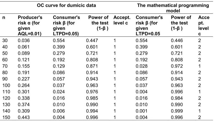
Table 1 showed the power which calculated by the mathematical programming model comparing with the power which calculated when acceptance level is fixed (c=1) by OC curve in Dumicic et al. [7]. The power which calculated by the mathematical programming model is approximately the same as the power which calculated by OC curve in Dumicic et al. [7].
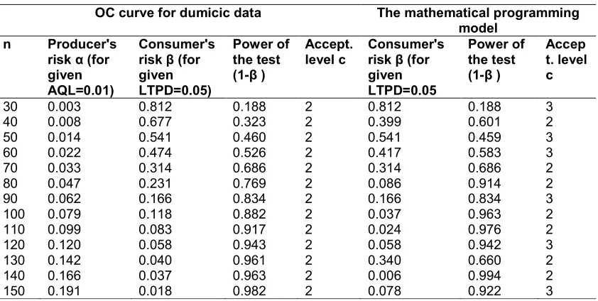
Table 2 showed the power which calculated by the mathematical programming model comparing with the power which calculated when acceptance level is fixed (c=2) by OC curve in Dumicic et al. [7]. The power which calculated by the mathematical programming model is approximately the same to the power which calculated by OC curve in Dumicic et al. [7].
Table 1. The power of test and acceptance level for the mathematical programming model by Elrefaey et al. [5] when c=1
OC curve for dumicic data The mathematical programming model
n Producer's risk α (for given AQL=0.01)
Consumer's risk β (for given LTPD=0.05)
Power of the test (1-β )
Accept. level c
Consumer's risk β (for given LTPD=0.05
Power of the test (1-β )
Acce pt. level c
30 0.036 0.554 0.447 1 0.554 0.446 2
40 0.061 0.399 0.601 1 0.399 0.601 2
50 0.089 0.279 0.721 1 0.279 0.721 2
60 0.121 0.192 0.808 1 0.192 0.808 2
70 0.155 0.129 0.871 1 0.028 0.972 1
80 0.191 0.086 0.914 1 0.086 0.914 2
90 0.227 0.057 0.943 1 0.057 0.943 2
100 0.264 0.037 0.963 1 0.037 0.963 2
110 0.301 0.024 0.976 1 0.004 0.996 1
120 0.338 0.016 0.985 1 0.016 0.984 2
130 0.374 0.010 0.990 1 0.010 0.990 2
140 0.309 0.006 0.994 1 0.001 0.999 1
Table 2. The power of test and acceptance level for the mathematical programming model by Elrefaey et al. [5] when c=2
OC curve for dumicic data The mathematical programming model
n Producer's risk α (for given AQL=0.01)
Consumer's risk β (for given LTPD=0.05)
Power of the test (1-β )
Accept. level c
Consumer's risk β (for given LTPD=0.05
Power of the test (1-β )
Accep t. level c
30 0.003 0.812 0.188 2 0.812 0.188 3
40 0.008 0.677 0.323 2 0.399 0.601 2
50 0.014 0.541 0.460 2 0.541 0.459 3
60 0.022 0.474 0.526 2 0.417 0.583 3
70 0.033 0.314 0.686 2 0.314 0.686 2
80 0.047 0.231 0.769 2 0.086 0.914 2
90 0.062 0.166 0.834 2 0.166 0.834 3
100 0.079 0.118 0.882 2 0.037 0.963 2
110 0.099 0.083 0.917 2 0.024 0.976 2
120 0.120 0.058 0.943 2 0.058 0.942 3
130 0.142 0.040 0.961 2 0.340 0.660 2
140 0.166 0.037 0.963 2 0.006 0.994 2
150 0.191 0.018 0.982 2 0.078 0.922 3
Table 3. The power, the level of significances and acceptance level for the suggested model
N Producer's risk α (for given AQL=0.01)
Consumer's risk β (for given LTPD=0.05)
Power of the test (1-β )
Acceptance level c
30 0.260 0.215 0.785 1
40 0.331 0.129 0.871 1
50 0.089 0.279 0.721 2
60 0.121 0.192 0.808 2
70 0.155 0.129 0.871 2
80 0.047 0.231 0.769 3
90 0.062 0.166 0.834 3
100 0.079 0.118 0.882 3
110 0.025 0.194 0.806 4
120 0.033 0.135 0.865 4
130 0.042 0.106 0.894 4
140 0.014 0.166 0.834 5
150 0.018 0.126 0.874 5
Tables 1 and 2 presented the acceptance level values which calculated by the mathematical programming model where the OC curve put it as fixed. The study explain the reason for the fixed number for acceptance level not realistic because it must be different when the sample size increase. That mean the mathematical programming can used to calculate efficiently the power and the acceptance level.
4.2 Second Application of the Suggested Nonlinear Goal Programming Model
The study used the suggested nonlinear goal programming model which presented in this
paper to determine Producer's risk (α) and consumer's risk (β) and acceptance number or level (c) simultaneously, while OC curve in acceptance sampling calculates Producer's risk (α) and consumer's risk (β) when acceptance number or level (c) is fixed.
The application takes the following steps:
This model used to determine the power of test (1- consumer's risk (β)), the level of significances (Producer's risk α) and the
acceptance number or level (c)
simultaneously.
respectively which used in Dumicic et al. [7].
Different sample sizes has been used, which given in Dumicic et al. [7], are mention in first column of Table 3.
Initial values 0.05 for level of significance is used.
Initial value 0.8 for the power of test (1-β) is used and it fixed for all cases.
GAMS statistical packages were used to solve the suggested nonlinear goal programming model for hypotheses tests. This model, takes the following form:
= + (9)
s.t
( , ) ∫ (1 − )
.
+ − = (10)
( , ) ∫ (1 − )
.
+ − = 1 − (11)
, , , ≥ 0
The following results are obtained in Table 3.
Table 3 presented the values for the power which calculated by the suggested nonlinear goal programming model depend on sample sizes, AQL (P0) and LTPD (P1) which are used in the OC curve in Dumicic et al. [7].
The power values which calculated in Table 3 can be divided the results to two cases. First: when sample sizes (30-70) are relatively small. Second: when sample sizes (80-150) are relatively large.
First: when the sample sizes (30-70) are relatively small, the values for the power which calculated are greater than the power values which calculated in the Tables 1 and 2.
Second: when the sample sizes (80-150) are relatively large, the values for the power which calculated are relatively less than the power values which calculated Tables 1 and 2.
That mean the results for the suggested nonlinear goal programming model is more logical and realistic.
The suggested nonlinear goal programming model calculated the Acceptance level or number c clearly. The suggested models can used in quality control application to make sample plan and calculate the acceptance level (c) more accurate in real application.Also the model
allowed α and β values to be free and determined their values more accurately which make balance between the power of a statistical test (1-β) and level of significance α. This enables decision makers in quality control to develop more accurate and free acceptance sampling plans.
5. CONCLUSION
The paper developed the mathematical
programming models presented by Elrefaey et al. [5] to nonlinear goal programming models for hypotheses tests. The paper introduced two nonlinear goal programming models for hypotheses tests. Then applied the previously models to the real quality control data from Dumicic et al. [7] to evaluate the efficiency of the suggested models with the real quality control data.
The results showed that the acceptance level values which calculated by the mathematical programming model and the suggested nonlinear goal programming models where the OC curve put it as fixed. The study explain the reason for the fixed number for acceptance level not realistic because it must be different when the sample size increase. That mean the suggested models can used to calculate efficiently the power and the acceptance level. The results also showed that the suggested nonlinear goal programming models calculated the Acceptance level or number c clearly. Also the model allowed α and β values to be free and determined their values more accurately which make balance between the power of a statistical test (1-β) and level of significance α. This enables decision makers in quality control to develop more accurate and free acceptance sampling plans.
COMPETING INTERESTS
Author has declared that no competing interests exist.
REFERENCES
1. Grant EL, Leavenworth RS. Statistical quality control. 7th Edition, McGraw-Hill, New York; 1996.
2. Montgomery DC. Introduction to statistical quality control. 7th Edition, John Wiley & Sons, Inc.; 2012.
4. Duarte BPM, Saraiva PM. An optimization‐based framework for designing acceptance sampling plans by variables for non‐conforming proportions. International Journal of Quality & Reliability Management. 2010;27(7):794-814.
5. Elrefaey AMM, Hamid R, Ismail EA, Ezzat
SM. Mathematical programming for
statistical inference. Asian Journal of Probability and Statistics. 2018;1(1):1-8. Article no.AJPAS.41012.
6. Juran JM, Godfrey AB. Juran's quality control handbook. 5th Edition, McGraw-Hill, New York; 1999.
7. Dumicic K, Vlasta Bahovec V, Zivadinovic NK. Analysing the shape of an OC curve for an acceptance sampling plan: A quality management tool. WSEAS Transactions
on Business and Economics. 2006;3(3): 169-177.
8. Schilling EG, Neubauer DV. Acceptance sampling in quality control. 4th Edition, Taylor & Francis Group, LLC. New York; 2017.
9. Mitra A. Fundamentals of quality control and improvement. 4th Edition, John Wiley and Sons, Inc.; 2016.
10. Ignizio JP. Goal programming and extensions. D.C. Health, Lexington, Massachusetts, U.S.A.; 1976.
11. Steuer RE. Multiple criteria optimization: Theory, computation and application. John Wiley, New York; 1986.
12. Rustem B. Algorithms for nonlinear programming and multiple - objective decision. John Wiley and Sons, Inc., New York; 1998.
© 2019 Ezzat; This is an Open Access article distributed under the terms of the Creative Commons Attribution License (http://creativecommons.org/licenses/by/4.0), which permits unrestricted use, distribution, and reproduction in any medium, provided the original work is properly cited.
Peer-review history: