R E S E A R C H A R T I C L E
Open Access
Discrimination-based sample size calculations
for multivariable prognostic models for
time-to-event data
Rachel C. Jinks, Patrick Royston
*and Mahesh KB Parmar
Abstract
Background: Prognostic studies of time-to-event data, where researchers aim to develop or validate multivariable prognostic models in order to predict survival, are commonly seen in the medical literature; however, most are performed retrospectively and few consider sample size prior to analysis. Events per variable rules are sometimes cited, but these are based on bias and coverage of confidence intervals for model terms, which are not of primary interest when developing a model to predict outcome. In this paper we aim to develop sample size recommendations for multivariable models of time-to-event data, based on their prognostic ability.
Methods: We derive formulae for determining the sample size required for multivariable prognostic models in time-to-event data, based on a measure of discrimination,D, developed by Royston and Sauerbrei. These formulae fall into two categories: either based on the significance of the value ofDin a new study compared to a previous
estimate, or based on the precision of the estimate ofDin a new study in terms of confidence interval width. Using simulation we show that they give the desired power and type I error and are not affected by random censoring. Additionally, we conduct a literature review to collate published values ofDin different disease areas.
Results: We illustrate our methods using parameters from a published prognostic study in liver cancer. The resulting sample sizes can be large, and we suggest controlling study size by expressing the desired accuracy in the new study as a relative value as well as an absolute value. To improve usability we use the values ofDobtained from the literature review to develop an equation to approximately convert the commonly reported Harrell’sc-index toD. A flow chart is provided to aid decision making when using these methods.
Conclusion: We have developed a suite of sample size calculations based on the prognostic ability of a survival model, rather than the magnitude or significance of model coefficients. We have taken care to develop the practical utility of the calculations and give recommendations for their use in contemporary clinical research.
Keywords: Prognostic modelling, Sample size, Survival data, Multivariable models
Background
Prognosis is one of the central principles of medical practice. Understanding the likely course of a disease or condition is vital if clinicians are to treat patients with confidence or any degree of success. No two patients with the same diagnosis are exactly alike, and the differences between them – e.g. age, sex, disease stage, genetics – may have important effects on the course their disease will take. Such characteristics are called ‘prognostic factors’,
*Correspondence: [email protected]
MRC Clinical Trials Unit at UCL, Aviation House, 125 Kingsway, London, WC2B 6NH, UK
and this phrase is usually taken to mean a factor which influences outcome independently of treatment.
For most applications, a single predictor is not suffi-ciently precise; rather a multivariable approach to progno-sis is required. Multivariable prognostic research enables the development of tools which give predictions based on multiple important factors; these are variously called prognostic models, prediction models, prediction rules or risk scores [1]. Such research also means that potential new prognostic factors are investigated more thoroughly, as it allows the additional value of the factor, above and beyond that of existing variables, to be established [1].
The majority of prognostic research is done retrospec-tively, simply because results are obtained much more quickly and cheaply by using existing data. In their 2010 review, Mallett et al. [2] found that 68 % of the 47 prog-nostic studies using time-to-event data included were retrospective. Altman [3] conducted a review of publi-cations which presented or validated prognostic mod-els for patients with operable breast cancer, and found that of the 61 papers reviewed, 79 % were retrospective studies. Disadvantages to retrospective studies include missing data, a problem which in general cannot be mit-igated by researchers. In addition, the assumption that data are missing at random may be implausible in such datasets, biasing results [4]. This is particularly true with stored samples, for example McGuire et al. [5] report that tumour banks usually contain a disproportionate num-ber of samples from larger tumours, which may introduce bias. Existing datasets may also contain many more can-didate variables than are really required to develop a good model, which can lead to multiple testing problems and a temptation to ‘dredge’ the data [6].
The best way to study prognosis is in a prospective study, which ‘enables optimal measurement of predictors and outcome’ [1]. However, a hurdle to designing good quality prognostic studies – whether prospective or retro-spective – is ensuring that enough patients are included in order that the study has the required precision of results. In the second of a series of papers on prognosis research strategies, Riley et al. [7] stress that in particular, studies aiming to replicate or confirm prognostic factors should ‘incorporate a suitable sample size calculation to ensure adequate power to detect a prognostic effect, if it exists’. Sample size is always an important issue for clinical stud-ies; however, little research has been performed which pertains specifically to the sample size requirements of multivariable prognostic studies. In his review of 61 pub-lications concerning breast cancer models, Altman [3] found that none justified the sample size used; and for many it was impossible to discern the number of patients or events contributing to the final model. Mallett et al. [2] found that although 96 % of studies in their review of survival models reported the number ofpatientsincluded in analyses, only 70 % reported the number ofevents– a key quantity for time-to-event data. In the same review, 77 % of the studies included did not give any justification for the sample size used. It is perhaps unsurprising that most papers reporting prognostic research do not justify the sample sizes chosen, as little guidance is available to researchers on how many patients should be included in prognostic studies.
Calculations based on the standard formula for the Cox proportional hazards (PH) model [8] are available for the situation where just one variable is of primary interest, but other correlated variables need to be taken
into account in the analysis [9–11]. For the more com-mon scenario where researchers wish to produce a mul-tivariable prognostic model and all model variables are potentially equally important, basing sample size on the significance of numerous individual variables is likely to be an intractable problem. In this situation the most often cited sample size recommendation is the rule of ‘10 events per variable’ (EPV) which originated from two simula-tion studies [12, 13]. In these studies, exponential survival times were simulated for 673 patients from a real ran-domised trial with 252 deaths and 7 variables (36 EPV), and then the number of deaths were varied to reduce the EPV. The authors found that choosing a single min-imum value for EPV was difficult but that results from studies having fewer than 10 EPV should be ‘cautiously interpreted’ in terms of power, confidence interval cov-erage and coefficient estimation for the Cox model. A later simulation study found that in ‘a range of circum-stances’ having less than 10 EPV still provided acceptable confidence interval coverage and bias when using Cox regression, but did not directly consider the statistical power of analyses nor the variability of the estimates [14]. It is perhaps inevitable that these two papers are often cited to justify low sample sizes. Indeed, Mallett et al. [2] found in their review of papers reporting development of prognostic models in time-to-event data, that of the 28 papers reporting sufficient information to calculate EPV, 14 had fewer than 10 EPV.
between 1 and 29 uniformly distributed covariates. The authors found that in both the 64 and 185 event datasets, 5-year survival predictions from the Cox models became increasingly biased upwards as the EPV decreased. In both datasets, the average error was below 10 % when EPV >10, and below 5 % when EPV >20. For ’sick’ subjects – those at high risk of death – higher EPVs were required: EPV >20 was required to reduce the expected error to 10 %. This work suggests that an EPV of 20 may be considered a minimum if accuracy of predictions are important, how-ever as it is found within a National Institutes of Health report, it is not easily available and so seems to be sel-dom cited. Additionally, two papers considered the effect of sample size on Harrell’scindex. Ambler, Seaman and Omar [17] noted that the value of thecindex increased with the number of events, however this issue was not the main focus of the publication and so investigation of this aspect was limited in scope. Vergouwe et al. [18] consid-ered the number of events required for reliable estimation of thecindex in logistic regression models and suggested that a minimum of 100 events and 100 non-events be used for external validation samples, which is likely to be higher than 10 EPV in many datasets. However being based on binary data, the results are not directly comparable to the sample size issue in prognostic models of time-to-event data.
In this paper we aim to develop calculations based on the prognostic ability of a model in time-to-event data, as quantified by Royston & Sauerbrei’sDmeasure of prog-nostic ability. We first describe theDstatistic, and then present sample size calculations based on Dfor use in prognostic studies. Finally we give examples and describe suggested methods for increasing the practical usability of the calculations.
Methods
Royston & SauerbreiDmeasure
There are various discrimination based measures of prog-nostic ability available for models of time-to-event data. The measure we have chosen to develop our calculations is Royston and Sauerbrei’sDmeasure [19], which has been shown to have many good properties which are described below [20]. The most commonly used measure of prog-nostic ability is probably Harrell’sc index [21], however this measure has some disadvantages: it is affected by censoring [22] and has a scale which can be difficult to interpret. Acknowledging the popularity and prevalence of thecindex in the literature, we do consider the rela-tionship betweencandDto ensure our methods are more widely usable (see Section Appendix).
Dmeasures prognostic ability by quantifying the sepa-ration in observed survival curves between subgroups of patients with differing predicted risks.Dwas developed in the Cox model framework and is based on risk ordering;
thusDcan be calculated whether the prognostic tool out-puts a continuous prognostic index, prognostic groups, or is even a subjective rule. However, it is assumed that the prognostic index resulting from the model is Normally distributed (although this is an approximation in the case of a non-continuous prognostic index). The full deriva-tion ofDcan be found in Royston and Sauerbrei’s original paper [19], but briefly:
D=κσ∗,
whereσ∗is an estimate of the standard deviation of the prognostic index values (under the assumption of Nor-mality) andκ = √8/π 1.60, a constant used to give a direct interpretation toD, as follows.
Dhas an intuitively appealing interpretation as the log hazard ratio between two equal-sized prognostic groups formed by dichotomising the prognostic index at its median. D’s interpretation as a log hazard ratio means that it can be translated to a hazard ratio between equally sized prognostic groups; so aDof 1 corresponds to a haz-ard ratio of e1 = 2.7 and D = 2 to e2 = 7.4. This allows researchers familiar with hazard ratios of treatment effects (for example) to have some idea of the increase in risk across the prognostic index of the model for a partic-ular value ofD. As a log hazard ratio,Dcan theoretically take any value in the range (−∞,∞), but in real situa-tions it is likely to be much closer to zero. A literature search for published values ofDin a wide range of disease areas found that the highest value out of 101 reported was 3.44; the second highest was 2.8 [23].D= 0 implies that the selected model is useless for prediction, andD < 0 may arise when a model fitted to one dataset is validated on another, indicating that the original model was flawed in some way. Additionally,Dhas a functional relationship with a measure of explained variationR2D[19]. This rela-tionship is important as most researchers will be more familiar with the 0–100 % range ofR2in linear regression. As well as its interpretability and applicability to many types of prognostic model,Dhas many other properties which make it suitable for practical use. These include robustness to outliers, sensitivity to risk ordering, inde-pendence from censoring (provided the prognostic model has been correctly specified and the PI is approximately normally distributed), and an easily calculated standard error [19]. Also, since it takes into account the fit of the model to the outcome data, it can be used in a model val-idation context; a vital part of a good prognostic study. Working withR2D, Choodari-Oskooei et al. [20] found that it was sensitive to marked non-normality of the prognostic index, but despite this concluded that overall it was one of two best explained variation measures for quantifying pre-dictive ability (along with Kent and O’Quigley’sR2PM[24]). DandR2Dcan be calculated in Stata using the user-written
Sample size calculations
Introduction
To develop the required calculations we start from the results in Armitage and Berry’s book [26] (p186) for com-parison of the means of two independent groups, with equal within-group variance. In this normal errors case, we consider two meansx1andx2measured in populations
of sizen1andn2respectively, wheres2is the within-group
variance of the response variable in both populations. The standard error of the difference inx1andx2is given by
SE(x1−x2)=
s2
1 n1+
1 n2
.
From this, various sample sizes can be calculated. Ifn1,
x1 and s2 are known, and it is desired that a difference
of x1 − x2 = δ will be just significant at the required
two-sidedαlevel with power 1−β, then the sample size required in the second population is
n2=s2
δ z1−α/2+z1−β
2 − s2
n1
−1
, (1)
where zx is the x-quantile of the standard normal distribution.
We can also calculate sample size in a different way, bas-ing it instead on the confidence interval of the estimated quantityδ. In order that the new estimate ofx2will have
a 100(1−α)% confidence interval of half width w, the sample size required is
n2=s2
w z1−α
2 − s2
n1
−1
. (2)
We can work from the same ideas to develop sample size calculations based onD, as this quantity is also normally distributed [23]. Consider the scenario where estimates ofDandSE(D)are available from a previous study using the same model, and researchers wish to validate the esti-mate of Dfor the model in a new study. LetD1be the
value of Din the first study,σ12the variance of D1, and
e1the number of events in the first study. LetD2be the
Dvalue in the (proposed) second study with e2 events,
andσ22= var(D2). The standard error ofD1−D2is thus
σ2
1 +σ22. As this does not explicitly includee1ande2we
must make an assumption about the relationship between the variance ofDand the number of events in the study in order to obtain sample size calculations.
The quantityλ
To develop the calculations required, we make a propor-tionality assumption. This is that for a given model with a certain ‘true’ value ofD, the ratio of the variancesσ12,σ22of
Din two datasets with differing numberse1,e2of events
(but sampled from the same distribution of covariates) equals the reciprocal of the ratio of the corresponding numbers of events:
σ2 1
σ2 2
= e2
e1.
This is reasonable, since the variance of a statistic is inversely related to the information in the data, which in a censored time-to-event sample is plausibly represented by the number of events [27]. We have shown through simulation and resampling that this assumption does hold reasonably well; and the larger the dataset, the better it holds (see [23], Tables 4.1 – 4.2).
Under the proportionality assumption we can write e1σ12=e2σ22=λ, whereλis a model- and disease-specific
structural constant which is incorporated in our calcula-tions. We can either estimateλby its value in a previous study (termedλs), or use an approximation incorporating a value ofDand the proportion of censoring (cens) in the dataset:
λm=c0+c1D1.9+c2(D·cens)1.3, (3)
where c0 = 2.66, c1 = 1.26, and c2 = −1.65. This
model was developed from simulated data and found to be reasonably accurate (see [23], Section 4.7.5).
Although our findings regardingλare approximations, this seems a reasonable price to pay when first con-structing a new method of planning prognostic studies. Prospective sample size calculations are by definition based on ‘guesstimated’ parameters, and these are not always checked post hoc, so in this respect we feel that the approximations made above are not inappropriate.
A note on the standard error of D
We have found that the default estimate of the standard error ofDoutput by thestr2dStata command tends to underestimate the true value (see [23], Section 3.3 for full details). The negative bias increases the higherDis; for example, whenD=0.8 simulation studies using different combinations of dataset size and proportion of censoring showed that the relative bias varied between 0 and –8 %, whereas whenD = 3.2, it varied from –17 % to –24 %. As an estimate of the standard error ofDis required to obtainλs, a downward bias in this quantity could reduce the required sample size and lead to underpowering.
Obtaining the sample size calculations
By applying this proportionality assumption, we can now
write the standard error ofD1−D2as
σ2
1 +λ/e2which,
using the same rearrangement as above, leads us to the fol-lowing two calculations. Firstly, to detect a difference inD between the first and second studies ofδwith significance levelαand power 1−β:
e2=λ
δ
zz 2
−σ2 1
−1
, (A)
wherezz = z1−α/2+z1−β for a two-sided (superiority)
αandzz=z1−α+z1−β for a one-sided (non-inferiority)
test. Secondly, in order that the estimate ofD1−D2has a
100(1−α)% confidence interval of half widthw
e2=λ
w z1−α
2 −σ2
1
−1
. (C)
By comparing (A) and (C) with (1) and (2) we can see there is an analogy between the common within-sample variances2and the quantityλ.
Note that unlike in typical sample size calculations, here the value ofσ12is available from the first study. Sincee2
must be positive, this places a lower limit onδandwfor these calculations:δ > σ1zz, andw> σ1z1−α. Having cal-culated minimumδ for various datasets, we feel that in general (A) and (C) are not very useful in practice and so do not consider them further. Instead we develop slightly different calculations which are described below.
Significance based calculations
Instead of estimating a value ofD1and its standard error
from a previous study, we pick a fixed target value ofD that we callD∗and assume this has zero uncertainty; so σ2
1 =0. Thus (A) becomes
e2=λ
δ
zz −2
(B)
We further obtain two calculations from (B) which are defined by how λ is estimated. Substituting λs into (B) gives us (B1), while substitutingλmgives us (B2):
e2=λs δ
zz −2
(B1)
e2=λm δ
zz −2
. (B2)
For a one-sided testH0 : D∗−D2 ≥ δandHA : D∗− D2 ≤δ. For a two-sided testH0 :D∗−D2= δandHA: D∗−D2=δ. If a previous study does exist, then either (B1)
or (B2) can be used. If no previous study exists, then (B1) cannot be used asλs cannot be calculated. When using (B1) and (B2)δhas a lower bound of zero.
One major benefit of usingλmis that using this approx-imation, different values ofDandcenscan be input which enables calculation of a range of sample sizes. This may be helpful in study planning where the value ofDand likely censoring proportion in the new study is uncertain.
Confidence interval based calculations
We can alter calculation (C) under the same assumption of a fixed targetDwhich we callD∗, as for (B1) and (B2). The confidence interval is thus around the quantityδ = D∗−D2. However, asD∗is assumed to have zero variance,
var(D∗−D2)=var(D2); so the width of CI forδ=D∗−
D2is equivalent to the width of CI forD2only.
Thus to estimate Din a new study with a confidence interval of half widthw, we replaceσ12with 0 in calculation (C), so the number of events required is
e2=λ
w z1−α/2
−2
(D)
Again substituting eitherλsorλmwe get
e2=λs
w z1−α/2
−2
(D1)
e2=λm
w z1−α/2
−2
(D2)
The only limit onwwhen using calculations (D1) and (D2) is that it must be>0.
Note that Eqs. (D) and (B) are equivalent if the power in (B) is 50 % andαis two-sided. So, for example, a study designed to estimateDwith a 95 % confidence interval of half width 0.2 requires the same number of patients as a study designed such that a difference inDofδ=0.2 from the target value is significant at the (two-sided) 5 % level with 50 % power.
Results
Validating the calculations
if the value ofD, or the censoring proportion, in the new study is larger than it was in the previous study, results in the new study may be less precise than were expected [23]. Equally if the values are smaller in the new study, results may be more precise than planned.
Implementation of commands in Stata
We have written two commands in Stata to implement the four calculations described here.dsampsi sig cal-culates the sample sizes required by (B1) and (B2), while
dsampsi cicalculates (D1) and (D2). These are avail-able from the author upon request.
Absolute and relative precision
AsDincreases, or ascensincreases, the number of events required to retain the same precision increases. This means that if the observed values of these two quanti-ties in the finished study are different to those used in the calculations, the estimate ofDin the final study will have higher or lower precision than was planned. This inadvertent under- or over-powering is a potential prob-lem in any sample size calculation for survival outcomes, including randomised clinical trials: any divergence from the expected censoring rate or hazard ratio for trial treat-ment would mean that the original sample size was either too large or too small; however, post-hoc calculations of power are not routinely performed. As the sample sizes output by our calculations are often high, the conse-quences of this under- or over-powering may be serious for prospectively planned prognostic studies: either many more patients are recruited than were really required, or a study does not meet its aims despite a large sample size.
In an effort to mitigate this problem, we present a prag-matic method to try and minimise the risk of serious under- and over-powering when using (B2) and (D2). Essen-tiallyδorware specified as a proportion ofDrather than as an absolute value, formalising the idea that ifDturns out to be higher than expected, researchers may be happy with a lower absolute precision than initially proposed.
If we denote bypthe proportion of the targetDthat we will accept as ourδorw, then calculations (B2) and (D2) become
e=λm
pD zz
−2
(4)
e=λm
pD z1−α/2
−2
, (5)
whereDis the best estimate available.
It is clear that for calculations (4) and (5), aspincreases the number of events required decreases. Also, it is impor-tant to observe that asDincreases, the number of events required decreases, which means we now have the reverse problem to previously: weloseprecision if the value ofD
is lower than expected. A straightforward solution is to combine the two approaches in a ‘composite’ sample size; specify both an absolute and a relative precision forδorw. For example, for a significance-based calculation we may be happy with precision of eitherδ = 0.15 orp = 10 % ofD, whichever requires the smaller sample size at each value ofD. We illustrate this strategy further below with real data examples.
Examples using parameters from a published paper
To illustrate the calculations we recommend as well as our composite sample size proposal, we use as a basis for our examples a paper published in 2008 which compared three existing staging systems for advanced liver cancer [28]. In this study the CLIP prognostic model was found to be most recommended, withD = 1.01. The standard error ofDwas given as 0.09, and the models were assessed on a dataset of 538 patients with 502 events (7 % censoring).
Calculations (B1) and (D1)
Let us first assume that we wish to validate the CLIP model on new data. Our objective is to have assurance of a certain level of performance (discrimination) of the CLIP model, as measured byD. Calculations (B1) and (D1) requireλto be estimated from the previous dataset; from the reported results in the paper,λs=e1σ12=502∗0.092=4.1.
Note that here we assume that the case mix of the vali-dation study is identical to the development study; if this is not the case then the interpretation of the value of D(or, indeed, any other model performance measure) at external validation is more complex [29, 30].
If we require a significance based non-inferiority study with one-sidedα= 0.05, 90 % power and non-inferiority margin δ = 0.25, 558 events are required according to calculation (B1). If it is expected that the same censor-ing proportion will hold in the new study, 601 patients should be recruited. For a study with two-sidedα = 0.05 (all other parameters held equal) 684 events are required. Figure 1 shows how the number of events required by calculation (B1) changes withδ, for a one-sided test.
If instead of a significance based calculation we wish to specify the CI forDin the new study, then we use (D1). In order that our estimate ofD in the new study has a 95 % confidence interval with half-width 0.2, we require 391 events. Figure 1 shows the effect ofwon the sample size calculation (D1).
Calculations (B2) and (D2)
Fig. 1Variation in events required by (left) calculation (B1) vsδ; (right) calculation (D1) vsw
To determine a target value ofD, we note that the paper in question reportedD=1.01 for the CLIP model, which is equivalent toR2D=19 % [19]. If we believe that the new factor will increase the proportion of variation explained by the model by 10 % (absolute) toR2D =29 %, our target value ofDshould beD=1.3. If we expect the censoring proportion to be 10 %, slightly higher than the CLIP paper, then using (3) we estimateλm=4.62.
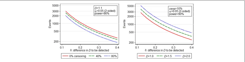
Under calculation (B2), 633 events are required for a non-inferiority study with one-sidedα=0.05, 90 % power and non-inferiority marginδ = 0.25. For the equivalent superiority study with two-sided α = 0.05, 777 events are required. Figure 2 shows the variation in number of events required by calculation (B2) for a two-sided test vs theδ desired, for different values ofDandcens. Note when looking at these graphs that although increasing cens decreases the number of events required, the total number of patients required increases.
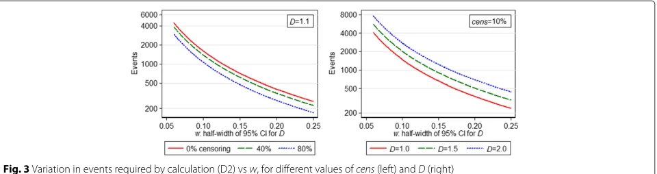
If a CI-based calculation is desired, in order that our estimate ofDin the new study has a 95 % confidence inter-val of half-width 0.2, using (D2) we require 444 events (usingλm=4.62). Figure 3 shows how required study size changes withD, censoring proportion andwaccording to calculation (D2).
Calculating a range of sample sizes
As already mentioned, by using λm we can calculate a range of sample sizes by inputting different likely values
of D and censoring proportion into Eq. (3). We briefly illustrate this using (D2).
We saw above that if we expectD= 1.3 and 10 % cen-soring in the new study, to obtain a 95 % CI forDwith half-width 0.2 we require 444 events (494 patients). If we believeDcould be as low as 1.1 or as high as 1.5, then inputting these values gives usλm = 4.08 andλ = 5.24 respectively, which results in sample sizes of 392 and 504 events (436 and 560 patients). If we think the censoring proportion might be as high as 30 % in the new study, then this results in aλm=4.25 and a sample size of 408 events ifD = 1.3: with 30 % censoring this means 583 patients are required. IfD=1.5 andcens=30 % thenλm =4.79 and 461 events are required; 659 patients.
Performing a range of calculations like this may help during study planning, and in assessing whether a retro-spective study might be large enough; and may be espe-cially useful when the value of Dand/or the censoring proportion in the study is uncertain.
Combining absolute and relative precision
As mentioned above, a pragmatic method for controlling power when the observed value ofDis not very certain is to define the desired precision with both absolute and relative limits. We illustrate this idea again using the CLIP paper example.
We return to the scenario outlined above to illustrate calculation (B2), but the same ideas hold for (D2). We once
Fig. 3Variation in events required by calculation (D2) vsw, for different values ofcens(left) andD(right)
again require a study with two-sidedα = 0.05 and 90 % power. Let us suppose that we are happy with precision of δabs = 0.25 or p = 20 % ofD, whichever requires the smaller sample size at each value ofD. The maximum sample size can be calculated by using calculation (B2): making δ the absolute value desired (0.25 in this exam-ple), and inputting D = δabs/p in the equation forλm (D = 0.25/0.2 = 1.25 in this example). Here this gives λm=4.47 and a required sample size of 753.
Figure 4 shows the sample size curves for the absolute and relative precisions, and the resulting profile for the smallest sample size is shown as a thick line, with a peak at D=1.25 where the number of events is 753. With a study of 753 events, if the value ofDin the new study turns out to beδ/p=1.25, then the study will have the correct pre-cision. As can be seen in Fig. 4, if the value ofDis either higher or lower than 1.25 then slightly more patients will have been recruited than strictly required, so the study will have slightly higher than anticipated precision. The precision that will actually be observed with a different value ofDcan be calculated by rearranging (B2) and sub-stituting the new value ofD. In this example, before the study we would anticipate that if D = 2, the smallestδ detectable with 90 % power and two-sidedα=5 % would
Fig. 4Events required by composite calculation (4) vsD, for absolute and relative values ofδ
be 0.4 (20 % of D = 2), however with 753 events it is actually 0.32.
Din practice
In order to use calculations (B2) and (D2), researchers must have in mind a target value of Dso that they can calculate λm. AlthoughD is becoming more commonly reported in prognostic research, it is not yet available for a wide variety of diseases, so it may be difficult to find a suitable value ofD. For this reason a literature search was carried out to assess how widelyDis used and to deter-mine its value in various disease areas. The main aim of the search was to show a method by which researchers might find a suitable value ofDfor use in their own work, but additionally the values found in the search may be used as a reference library by users of calculations (B2) and (D2). We also used some of the values collected to develop an equation to convert Harrell’sc-index toD. The meth-ods and results of the literature search are described in detail elsewhere [23]; we present the main findings here.
The search was divided into two parts: first a search for all reported values ofD, second a search for a limited num-ber of values of Harrell’sc-index. The former resulted in 108Dvalues reported in 34 separate papers; the latter 331 cvalues from 77 papers. We collated a dataset of models from the searches which had bothDandcvalues reported, and augmented these with values from models developed on publicly available time-to-event datasets (from books and papers). The 294 paired (D,c) values showed a strong relationship and we modelled this by simply fitting a frac-tional polynomial to the data, giving Eq. (6) which could be used by researchers to convert a value ofctoDfor use in our calculations.
D=5.50(c−0.5)+10.26(c−0.5)3 (6)
Figure 5 shows the data used to develop (6) overlaid with the model itself. Table 1 shows various points on the modelled relationship betweenDandc.
Fig. 5The (c,D) pairs used to model the relationship betweencand Dand the final model Eq. (6)
values were explored and grouped by disease area. Ulti-mately, we obtained 480 values ofDin total, ranging from 0 to 3.44 and with mean 1.40 (median 1.30). Of these, 296 values were from prognostic models (predicting a disease event in patients who already have the disease of interest) and 184 from risk models (predicting onset of a disease in healthy patients). We found that the mean value ofD amongst the prognostic models (D = 1.30) was slightly lower than for the risk models (D= 1.47). A full descrip-tion of theDvalues collected can be found in [23]. For most diseases only one or two papers were retrieved.
Discussion
Recommendations for practice
As argued above, we find that calculations based on (A) and (C) are of limited practical use because of the lower limits on the values ofδandwthat can be detected. Thus the calculations which we find most useful are (B1) and (B2) which are based on significance testing, and (D1) and (D2) which are based on the precision of the estimate ofD in the new study. It is purely down to the preferences of the
Table 1The relationship betweenc,DandR2D: selected points
c D R2D c D R2D
0.50 0.000 0.000 0.72 1.319 0.294 0.52 0.110 0.003 0.74 1.462 0.338 0.54 0.221 0.011 0.76 1.610 0.382 0.56 0.332 0.026 0.78 1.765 0.427 0.58 0.445 0.045 0.80 1.927 0.470 0.60 0.560 0.070 0.82 2.096 0.512 0.62 0.678 0.099 0.84 2.273 0.552 0.64 0.798 0.132 0.86 2.459 0.591 0.66 0.922 0.169 0.88 2.652 0.627 0.68 1.050 0.208 0.90 2.857 0.661 0.70 1.182 0.250 0.92 3.070 0.692
researcher as to which type is chosen. Within each type, there are two options depending on whether researchers wish to include information from a previous study in their calculation (B1, D1), or want to (or have no choice but to) choose target values for the parameters (includingD) instead (B2, D2). The latter option makes it easier to cal-culate a range of possible sample sizes, as shown in the example above. This may be important if researchers are not very confident about the likely values ofDthat will be seen in the new study, or wish to explore the effects of different censoring proportions. For this reason we would recommend (B2) and (D2) over (B1) and (D1) in most cases. However, if a reliable previous study exists then (B1) and (D1) may be preferred (for example, if researchers are seeking to validate an existing study). If (B1) or (D1) are used, we recommend that a bootstrap estimate of the stan-dard error ofDis used to calculateλsinstead of the default estimate provided, as this is likely to underestimate this quantity.
If (B2) or (D2) are chosen, a value of D and the censoring proportion for the proposed study must be estimated. Estimating the censoring proportion should be straightforward for researchers but finding a suitable value of Dmay be more problematic. If an appropriate value cannot be found in the library of values presented in [23], we recommend that researchers search litera-ture for a suitablec-index value and convert this instead using (6). The question of what is a ‘suitable’ value of either c or D, in terms of how similar the study pop-ulation, methods, model and other aspects must be, is difficult to answer and we do not attempt to give a solu-tion here. In the absence of any guidance whatsoever as to a suitable value of D, we suggest using a value of D = 1.4, the mean value ofDacross the large number of prognostic models collated here. We give a decision-making flowchart in Fig. 6 to help potential users of our method determine which calculations can be used in their situation.
Although the sample sizes output by the calculations tend to be large, we have given some suggestions on how study size can be managed, for example by considering precision as a proportion of the measure of interest, rather than (or as well as) a fixed value. We recommend using this method to prevent inadvertent loss of precision due to uncertainty around the estimated value ofDwhen using (B2) or (D2). However it is worth noting that this under-or over-powering is a potential problem in any scenario, including randomised clinical trials.
Conclusions
Fig. 6Flowchart to aid decision making
and they often use time-to-event data analysed with the Cox proportional hazards model. Many prognostic studies are performed with retrospective data and often without reference to sample size calculations [2], suggesting that obtaining reliable results from such studies may often be a matter of chance.
The main sample size guidance available to and used by researchers developing prognostic survival models is the events per variable (EPV) calculation with a lower limit of 10 EPV usually quoted; however, this idea is based on just two limited simulation studies. These studies con-centrated on the significance of model coefficients, which is of secondary importance in a prognostic model to be used for outcome prediction. In this paper we have pre-sented some sample size calculations based instead on the discrimination ability of a survival model, quantified by Royston and Sauerbrei’s Dstatistic. We have also given some suggestions and methods for improving the practical use of the calculations in research.
Due to the novel nature of the methods presented in this paper, there are limitations to the work described here and further avenues yet to be explored. In particular, we note that the sample size calculations presented here pay no attention to the number of variables to be explored. From previous work we know that the number of candidate vari-ables for a model can have an effect on the estimate ofD in some situations [23]. If a model is developed using an automatic variable selection method and then validated in the same dataset, then increasing the number of candidate
variables increases the optimism present in the estimate of D; however, we have not covered this issue here. Addition-ally, we acknowledge that changes in case mix between datasets can add complexity to defining improvement in the prognostic performance of a model, whether D or some other performance measure is used. The methods introduced in [29] may offer a solution to this problem but it is too early to say; in this paper we have made the assumption that the distributions of covariates are compa-rable between datasets used for model development and validation purposes.
We hope that these calculations, and the guidance pro-vided for their use, will help improve the quality of prog-nostic research. As well as being used to provide sample sizes for prospective studies in time-to-event data, they can also be used for retrospective research; either to give the required sample size before suitable existing data is sought, or to calculate the likely precision of results where a dataset has already been chosen. At the very least we hope that the existence of these calculations will encour-age researchers to consider the issue of sample size as a matter of course when developing or validating prognostic multivariable survival models.
Appendix: simulation studies to test sample size calculations
The sample size calculations were tested using simulation, to check that they provided the desired power andα, or the desired confidence interval width.
Table 2Results of simulation study to test (B1) and (B2)
Simulation parameters Observed (B1) Observed (B2)
β D power δ cens e2 % type 1 (se) % power (se) e2 % type 1 (se) % power (se)
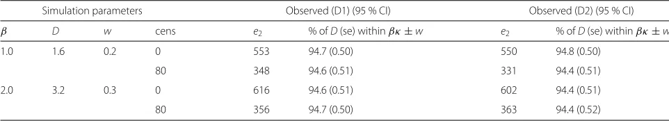
Table 3Results of simulation study to test (D1) and (D2)
Simulation parameters Observed (D1) (95 % CI) Observed (D2) (95 % CI) β D w cens e2 % ofD(se) withinβκ±w e2 % ofD(se) withinβκ±w
1.0 1.6 0.2 0 553 94.7 (0.50) 550 94.8 (0.50)
80 348 94.6 (0.51) 331 94.4 (0.51)
2.0 3.2 0.3 0 616 94.6 (0.51) 602 94.4 (0.51)
80 356 94.7 (0.50) 363 94.4 (0.52)
We simulated time-to-event data from an exponential distribution, with baseline cumulative hazard functionH0,
using the method described by Bender et al. [31]. The sur-vival time for the proportion hazards (PH) model with regression coefficients (log hazard ratios)βand covariate vectorXwas simulated using
Ts=H0−1[−log(U)exp(−βX)] (7)
whereU ∼ U[ 0, 1]. Since simulating a full multivariable vector is complex both computationally and in terms of interpretation, we instead used a surrogate scalarX.Xwas simulated as∼ N(0, 1), and the value ofβ fixed, so that the resulting prognostic indexβX was also normal. In a dataset simulated this way,D=βκ[23].
We simulated random non-informative right-censoring using the same method to obtain an exponentially dis-tributed censoring timeTcfor each patient; noteTcwere not dependent on X. Records where Tc < Ts were considered censored at time Tc. The desired censoring proportion was achieved by changing the baseline hazard. Throughout our simulations we wished to use datasets with an exact number of events and censoring proportion. To obtain a dataset with exactlye1events and exact
cen-soring proportioncens, we first generated a dataset with 2( e1
1−cens)records and approximate censoring proportion cens. We then simply randomly selectede1records ending
in failure, and e1
1−cens −e1censored records, to form the final dataset.
The variance or standard error of Dwas obtained by bootstrap whenever required.
Calculations (B1) and (B2)
For (B1) the first step of the simulation is to generate a ‘first’ study withe1/(1− cens) records and exactly e1
events. This dataset is bootstrapped to obtainσ12, the vari-ance ofD, and thenλsis calculated from this quantity and e1. For (B2) the first step is to calculate λmfrom Eq. (3) with the desired estimates ofDand cens.
The next steps are common to both (B1) and (B2) once e2 is calculated. Datasets of the required size are
gener-ated separately under the null and alternative hypotheses, and bootstrapped to obtainse(D). The whole procedure is repeated 2000 times for each combination of parameters varied (D, power,δand cens), and test statistics calculated
to determine if the number of eventse2gives the required
power and type 1 error. A selection of results is given in Table 2. For (B1), this table shows the results fore1=750;
the simulations were repeated fore1 =1500 and showed
very similar results but these are not presented here.
Calculations (D1) and (D2)
As for (B1), the first step of the simulation study for (D1) is to generate a ‘first study’ to provide values ofe1andσ12
for the calculation ofλs.
For (D2) λm is calculated using Eq. (3). For both (D1) and (D2), oncee2has been calculated, a dataset with the
required number of events and censoring proportion is simulated andDcalculated. This was repeated 2000 times for each combination of parameters. The proportion of repetitions for which the estimate ofDis withinwof the inputD = βκ gives the % CI which has width±w. This should approximate 1−α, if the sample size calculation and estimation ofλare correct. A selection of results is given in Table 3. For (D1), this table shows the results for e1=750; the simulations were repeated fore1=1500 and
showed very similar results but these are not presented here.
Competing interests
The authors declare that they have no competing interests.
Authors’ contributions
All authors developed the methodology. RJ carried out the statistical analysis, simulation studies and literature searching for theDlibrary, and drafted the manuscript. PR and MP input into the manuscript. All authors read and approved the final manuscript.
Acknowledgements
We thank Tim Morris and Babak Oskooei for their helpful comments and suggestions. This work was supported by UK Medical Research Council Hub for Trials Methodology Research budget A735-5QP21.
Received: 6 November 2014 Accepted: 2 October 2015
References
1. Moons KG, Royston P, Vergouwe Y, Grobbee DE, Altman DG. Prognosis and prognostic research: what, why, and how? BMJ. 2009;338:1317–20. 2. Mallett S, Royston P, Dutton S, Waters R, Altman DG. Reporting
methods in studies developing prognostic models in cancer: a review. BMC Med. 2010;8:20+.
4. Altman DG, Lyman GH. Methodological challenges in the evaluation of prognostic factors in breast cancer. Breast Cancer Res Treat. 1998;52(1-3): 289–303.
5. McGuire WL. Breast cancer prognostic factors: evaluation guidelines. J Natl Cancer Inst. 1991;83(3):154–5.
6. Royston P, Moons KG, Altman DG, Vergouwe Y. Prognosis and prognostic research: developing a prognostic model. BMJ. 2009;338:1373–7. 7. Riley RD, Hayden JA, Steyerberg EW, Moons KGM, Abrams K, Kyzas PA,
et al. For the PROGRESS group: Prognosis research strategy (PROGRESS) 2: Prognostic factor research. PLoS Med. 2013;10(2):e1001380+.
8. Schoenfeld DA. Sample-size formula for the proportional-hazards regression model. Biometrics. 1983;39(2):499–503.
9. Schmoor C, Sauerbrei W, Schumacher M. Sample size considerations for the evaluation of prognostic factors in survival analysis. Stat Med. 2000;19(4):441–452.
10. Bernardo MVP, Lipsitz SR, Harrington DP, Catalano PJ. Sample size calculations for failure time random variables in non-randomized studies. J R Stat Soc (Series D): The Statistician. 2000;49:31–40.
11. Hsieh F, Lavori PW. Sample-size calculations for the Cox proportional hazards regression model with nonbinary covariates. Control Clin Trials. 2000;21(6):552–60.
12. Concato J, Peduzzi P, Holford TR, Feinstein AR. Importance of events per independent variable in proportional hazards analysis. I. Background, goals, and general strategy. J Clin Epidemiol. 1995;48(12):1495–1501. 13. Peduzzi P, Concato J, Feinstein AR, Holford TR. Importance of events per
independent variable in proportional hazards regression analysis. II. Accuracy and precision of regression estimates. J Clin Epidemiol. 1995;48(12):1503–10.
14. Vittinghoff E, McCulloch CE. Relaxing the rule of ten events per variable in logistic and Cox regression. Am J Epidemiol. 2007;165(6):710–8. 15. Copas JB. Regression, prediction and shrinkage. J R Stat Soc Ser B
Methodol. 1983;45(3):311–54.
16. Smith LR, Harrell FE, Muhlbaier LH. Problems and potentials in modeling survival. In: Grady ML, Schwartz HA, editors. Medical Effectiveness Research Data Methods (Summary Report) AHCPR publication, no. 92-0056. US Dept of Health and Human Services, Agency for Health Care Policy and Research; 1992. p. 151–159.
17. Ambler G, Seaman S, Omar RZ. An evaluation of penalised survival methods for developing prognostic models with rare events. Stat Med. 2012;31:1150–61.
18. Vergouwe Y, Steyerberg EW, Eijkemans MJ, Habbema JDF. Substantial effect sample sizes were required for external validation studies of predictive logistic regression models. J Clin Epidemiol. 2005;58:475–83. 19. Royston P, Sauerbrei W. A new measure of prognostic separation in
survival data. Stat Med. 2004;23(5):723–48.
20. Choodari-Oskooei B, Royston P, Parmar MK. A simulation study of predictive ability measures in a survival model. Stat Med. 2012;31(23): 2627–43.
21. Harrell FE, Lee KL, Califf RM, Pryor DB, Rosati RA. Regression modelling strategies for improved prognostic prediction. Stat Med. 1984;3(2):143–52. 22. Gönen M, Heller G. Concordance probability and discriminatory power in
proportional hazards regression. Biometrika. 2005;92(4):965–70. 23. Jinks RC. Sample size for multivariable prognostic models: PhD thesis,
University College London; 2012.
24. Kent JT, O’Quigley J. Measures of dependence for censored survival data. Biometrika. 1988;75(3):525–34.
25. Royston P. Explained variation for survival models. Stata J. 2006;6:1–14. 26. Armitage P, Berry G, Matthews JN. Statistical Methods in Medical
Research, 4th ed. Oxford: Blackwell Science; 2001.
27. Volinsky CT, Raftery AE. Bayesian Information Criterion for Censored Survival Models. Biometrics. 2000;56:256–62.
28. Collette S, Bonnetain F, Paoletti X, Doffoel M, Bouché O, Raoul JL, et al. Prognosis of advanced hepatocellular carcinoma: comparison of three staging systems in two French clinical trials. Ann Oncol. 2008;19(6): 1117–26.
29. Vergouwe Y, Moons KGM, Steyerberg EW. External validity of risk models: use of benchmark values to disentangle a case-mix Effect from incorrect coefficients. Am J Epidemiol. 2010;172(2):971–80.
30. Steyerberg EW. Clinical Prediction Models: A Practical Approach to Development, Validation, and Updating (Statistics for Biology and Health), 1st ed.: Springer; 2008.
31. Bender R, Augustin T, Blettner M. Generating survival times to simulate Cox proportional hazards models. Stat Med. 2005;24(11):1713–23.
Submit your next manuscript to BioMed Central and take full advantage of:
• Convenient online submission
• Thorough peer review
• No space constraints or color figure charges
• Immediate publication on acceptance
• Inclusion in PubMed, CAS, Scopus and Google Scholar
• Research which is freely available for redistribution