Available Online at www.ijpret.com 657
INTERNATIONAL JOURNAL OF PURE AND
APPLIED RESEARCH IN ENGINEERING AND
TECHNOLOGY
A PATH FOR HORIZING YOUR INNOVATIVE WORKPGSLDA- BASED FACE DETECTION
MR. A. S. CHHAJED, DR. MS. K. C. JONDHALE
Computer Sci. and Engg. Department, SRTMU, Nanded.
Accepted Date: 05/03/2015; Published Date: 01/05/2015
\
Abstract:Face detection is to determine whether or not there are any faces in an image and if present, then mark face location. Face detection has many computer vision applications. Face detection is a challenging task in computer vision and pattern recognition. There has been much progress in frontal face detection in recent years. Various face detection methods are available in literature. Most of the face detectors use appearance based method. This paper deals with the algorithm for automatic face detection using Parallel Greedy Sparse Linear Discriminant Analysis (PGSLDA) which is capable of processing images speedily and achieving high detection rates. Face detection using PGSLDA method is done in three steps. The first step is preprocessing, the introduction of a new image representation called the “Integral Image” which allows the Haar features used by our detector to be computed very quickly for each node at constant time. The second step is feature selection/extraction method. Linear Discriminant Analysis (LDA) classifier had used. LDA uses class-separability criterion, which selects maximum eigen value as threshold which discriminate face class from nonface class. It is also useful in asymmetric data. The third step is to arrange LDA weak classifiers in coarse-to-fine cascaded manner gives high detection rate with computationally efficient. We have proposed PGSLDA methods which combine specific and sensitive classifiers in a hybrid parallel manner. In which classifiers located near the beginning of the cascade are used more frequently than subsequent classifiers. It gives 94% accuracy with 0.28% false positive rate. These experimental results show that the combination of classifier in hybrid parallel manner which improve the performance as compare to cascade.
Keywords: Integral Image, Face Detection, Greedy Sparse Linear Discriminant Analysis (GSLDA), Feature Selection, Cascade Classifier
Corresponding Author: MR. A. S. CHHAJED
Access Online On:
www.ijpret.com
How to Cite This Article:
A. S. Chhajed, IJPRET, 2015; Volume 3 (9): 657-673
Available Online at www.ijpret.com 658
INTRODUCTION
Face detection is to determine whether or not there are any faces in the image and if present, return the image location and extent of each face. An ideal face detection system should be able to identify and locate all faces regardless of their positions, scale, orientation, lightning conditions, and expressions and so on. Due to the large intra-class variations in facial appearances, face detection has been a challenging problem in the field of computer vision. Face detection is the first processing stage in a face-recognition system. Human face detection by computer systems has become a major field of interest. Face detection algorithms has been used in a wide range of applications, such as security control, video retrieving, biometric signal processing, human computer interface, face recognitions and image database management, intelligent video surveillance, vision based teleconference systems and human motion analysis [2]. Face detection is challenging due to large variations of the visual appearances, poses and illumination conditions. Furthermore, face detection is a highly imbalanced classification task. A typical natural image contains many more negative background patterns than face patterns. The number of background patterns can be 100000 times larger than the number of object patterns [1]. That means if, one wants to achieve a high detection rate, together with a low false detection rate, one need to design a specific and sensitive classifier that takes the imbalanced data distribution into consideration.
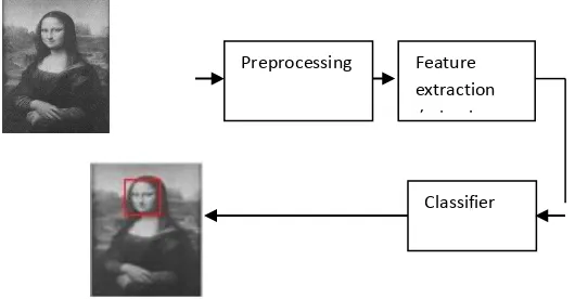
The generic face detection system is as shown in Figure 1.
Figure 1. Generic face detection system.
The function of each module is as follows:
1. Preprocessing: It is the process of manipulating an image so that the result is more suitable than the original for specific application. The image is pre-processed to remove noise. After
Preprocessing Feature extraction /selection
Available Online at www.ijpret.com 659 preprocessing it gives image that is more suitable for face detection. Different techniques available for preprocessing in face detection are as follows:
a. Image smoothing: Edges and sharp intensity transition (such as noise) can be removed by image smoothing using Lowpass filter.
b. Image sharpening: Edges can be detected in the frequency domain can be achieved by Highpass filter.
c. Histogram Equalization: Histogram is used to represent face statistics and training on multiple view samples. It is used to remove light and color normalization.
d. Integral image: To minimize the effect of different lightning conditions, all example images used for training were variance normalized. The variance of an image can be computed quickly using a pair of integral images, also it gives illumination normalization.
e. Size normalization: To remove bias from the detection results due to association of particular scale, position or orientation to a particular face.
f. Interpolation: Image interpolation is a basic tool used extensively in task such as zooming, shrinking, rotating, and geometric correction, scaling [26].
2. Feature extraction/selection: Feature extraction is a process to convert input data into relevant abstract information. There are many motivations for using features rather than the pixels directly. The most common reason is that features can act to encode ad-hoc domain knowledge that is difficult to learn using a finite quantity of training data, another reason is that the feature-based system operates much faster than a pixel-based system. Different feature extraction techniques available are: ICA, PCA, LDA etc.
3. Classifier: Classifier in face detection is a classification function 𝑓(𝑥) for the discrimination between face and non-face patterns. Given a feature set and a training set of face and nonface images, different machine learning approaches could be used to learn a classification function. A classification function takes features as input and defines how face areas can be discriminated from their backgrounds (nonface). Different classifiers available are: Neural network, SVM, AdaBoost, cascade, GSLDA etc.
Available Online at www.ijpret.com 660 system which achieves detection and false positive rates. Its ability to detect faces extremely rapidly. Operating on 640 by480 pixel images, faces are detected at 14 frames per second on a standard PC. Our system achieves high frame rates working only with the information present in a single grey scale image. These alternative sources of information can also be integrated with our system to achieve even higher frame rates. In order to compute these features very rapidly at many scales we introduce the integral image representation for images. The integral image can be computed from an image using a few operations per pixel. Once computed, any
one of these Haar-like features can be computed at any scale or location in constant time. The
second contribution of this paper is a method for constructing a classifier by selecting a small number of important features using LDA . The weak learner is constrained so that each weak classifier returned can depend on only a single feature. The third part is contribution of this paper is a method for combining successively simple to complex classifiers in a parallel structure which increases the speed of the detector by focusing attention on promising regions of the image. In the domain of face detection it is possible to achieve less than 1% false negatives and 40% false positives using a classifier constructed from five Haar-like features.
This paper is organized as follows: Section II, introduce Integral image representation with feature extraction method as LDA. Section III explain the proposed algorithm for training weak classifier and discuss its complexity. The results of numerous experiments are presented in Section IV. We conclude the paper in Section V.
I. FEATURE EXTRACTION METHOD
The GSLDA face detection algorithm had used as basis of our face detection. The algorithm checks specific Haar-like feature of human face. Threshold of each cascade classifier can be found by using GSLDA method [1]. When one of these feature is found, it pass decision stump to the next stage of detection.
The algorithm uses an integral image in order to process Haar-like features of a face candidate in constant time. It uses a cascade of node which is used to eliminate non-face candidates quickly. If all nodes are passed the face candidate is concluded to be a face. These terms will be discussed in more detail in the following sections:
A. Integral Image Representation
Available Online at www.ijpret.com 661 The integral image had computed from an image using a few operations per pixel. Once computed, any one of these Haar-like features can be computed at any scale or location in
constant time.
Rectangle features has computed very rapidly using an intermediate representation for the
image which is called integral image. The integral image at location x, y contains the sum of the
pixels above and to the left of x, y, inclusive:
𝑖𝑖(𝑥, 𝑦) = ∑ 𝑖(𝑥′, 𝑦′) 𝑥′≤𝑥,𝑦′≤𝑦
(1)
Where, 𝑖𝑖(𝑥, 𝑦) is the integral image,
𝑖(𝑥, 𝑦) is the original image.
Integral image calculation is also representing as the following pair of recurrences:
𝑠(𝑥, 𝑦) = 𝑠(𝑥, 𝑦 − 1) + 𝑖(𝑥, 𝑦)
𝑖𝑖(𝑥, 𝑦) = 𝑖𝑖(𝑥 − 1, 𝑦) + 𝑠(𝑥, 𝑦) (2)
Where, 𝑠(𝑥, 𝑦) is the cumulative row sum, 𝑠(𝑥, −1) = 0,and 𝑖𝑖(−1, 𝑦) = 0).
Figure 2. Integral image calculation [3].
As shown in figure 2, the sum of the pixels within rectangle D can be computed with four array references. The value of the integral image at location 1 is the sum of the pixels in rectangle A. The value at location 2 is A+B, at location 3 is A+C, and at location 4 is A+B+C+D. The sum within D can be computed as 4+1-(2+3) [4]. Using the integral image any rectangular sum can be computed in four array references. Clearly the difference between two rectangular sums can be computed in eight references. Since the two-rectangle features defined above involve adjacent rectangular sums they have computed in six array references, eight in the case of the three-rectangle features, and nine for four-three-rectangle features.
Available Online at www.ijpret.com 662 The simplicity of Haar-like features is the key to a success of [3] frontal face detector. However, the features are not discriminative enough to distinguish more complex object. Numerous researchers had introduced more types of wavelets to extend Haar- like’s discriminative power.
1) Haar Wavelet
Wavelets provide a natural mathematical structure for describing patterns; a more detailed treatment can be found in Mallat (1989).
Figure 3. Haar wavelet frameworks [5].
Figure 3 (A) the Haar scaling function and wavelet, (B) the three types of 2-dimensional non-standard Haar wavelets: vertical, horizontal, and diagonal, and (C) the shift in the non-standard transform as compared to our quadruple dense shift resulting in an over complete dictionary of wavelets. The representation we use, Haar wavelets, identifies local, oriented intensity difference features at different scales and is efficiently computable. The Haar wavelet is perhaps the simplest such feature with finite support. In mathematics, the Haar wavelet is a sequence of rescaled "square-shaped" functions which together form a wavelet family or basis. Wavelet analysis is similar to Fourier analysis in that it allows a target function over an interval to be represented in terms of an orthonormal function basis. The Haar sequence is now recognized as the first known wavelet basis. We transform our images from pixel space to the space of wavelet coefficients, resulting in an overcomplete dictionary of features that are then used as training for a classifier.
More specifically, we use three kinds of features. The value of a two-rectangle feature is the difference between the sum of the pixels within two rectangular regions. The regions have the same size and shape and are horizontally or vertically adjacent (see Figure 4). A three-rectangle feature computes the sum within two outside rectangles subtracted from the sum in a center rectangle. Finally a four-rectangle feature computes the difference between diagonal pairs of
Available Online at www.ijpret.com 663 rectangle features is quite large, over 180,000. Note that unlike the Haar basis, the set of rectangle features is over complete [9].
Figure 4. Haar-like rectangle features have shown as above. The sums of the pixels which lie within the white rectangles are subtracted from the sum of pixels in the grey rectangles.
Two-rectangle features are shown in (A) and (B). Figure (C) shows a three-Two-rectangle feature, and (D) a four-rectangle feature.
Linear Discriminant Analysis
Fisher’s linear discriminant (FLD) has recently emerged as a more efficient approach for many pattern classification problems than traditional PCA. The ultimate goal in choosing a representation for a face detection system is finding one that yields high inter-class (face &nonface) variability, while at the same time achieving low intra-class variability. Since face classes of people can be quite complex, this is a nontrivial task.
Although PCA is efficient for data representation, it may not be good for class discrimination.
To find a feature vector w that separates classes, LDA maximizes the following criterion
function, Let us assume that we have a set of training patterns 𝑥 = [𝑥1, 𝑥2, … , 𝑥𝑀]𝑇
where each of which is assigned to one of two classes, 𝐶1 and 𝐶2. We can find a weight vector
𝒘 = [𝑤1, 𝑤2,…,𝑤𝑀]𝑇and a threshold θsuch that
𝑤𝑇𝑥 + θ ≥ 0 (𝑥𝜖𝐶1),
𝑤𝑇𝑥 + θ < 0 (𝑥𝜖𝐶
2) (1)
In general, we seek the vector [𝑤1, 𝑤2, … , 𝑤𝑀] best satisfies (eq.1). The data are said to be
linearly separable if for all 𝑥 (eq.1) is satisfied. An objective of a linear combination is the
Available Online at www.ijpret.com 664
proposed by Fisher is the ratio 𝑗(𝑤) of between-class to within-class variance should be a
maximum.
In this section, we begin by introducing the basic concept of classical linear discriminant analysis (LDA) and greedy sparse linear discriminant analysis (GSLDA).
j(w) = max 𝑤
𝑤𝑇𝑆 𝑏𝑤 𝑤𝑇𝑆
𝑤𝑤
𝑆𝑏 = ∑𝑐∈𝐶𝑁𝑐(𝑚𝑐 − 𝑚̅ )(𝑚𝑐− 𝑚̅ )𝑇,
𝑆𝑤 = ∑𝑐∈𝐶∑𝑥∈𝑐(𝑥 − 𝑚𝑐)(𝑥 − 𝑚𝑐)𝑇. (2)
Where,
𝐶1,𝐶2 - Positive class, negative class respectively
𝑁1, 𝑁2 - The number of training samples in first and second class respectively
𝑥 - The new instance being inserted
𝑚1, 𝑚2 - The mean of the first and second class respectively
𝑚̅ - The global mean of the training samples
𝑆𝑏 - Between class scatter matrix
𝑆𝑤- Within class scatter matrix
To find maximum of 𝐽(𝑤), we differentiate and equate to zero.
𝑑𝑤𝑑 𝐽(𝑤) = 𝑑 𝑑𝑤(
𝑤𝑇𝑆𝐵𝑤 𝑤𝑇𝑆
𝑤𝑤) = 0 (3)
The solution will be eigen vector(s )= 𝑠𝑤−1
Eigen vector of matrix 𝑠𝑤−1 is calculate as
Available Online at www.ijpret.com 665 Where,
𝑠𝑤−1-Inverse of within class scatter matrix,
I-Identity matrix, 𝜆 − Eigen value
Put maximum Eigen value (𝝀) in equation (𝟒) we get Eigen
Vector as discriminant feature. LDA has produced𝑪 − 𝟏. Feature set, where 𝑪 represents
number of classes. As shown in [21], for two-class problems, the computation can be made very efficient as the only finite eigenvalue can be computed in closed-form as with because in this case is a rank-one matrix is a column vector. Therefore, the computation is mainly determined
by the inverse of 𝑺𝒘 .When a greedy approach is adopted to sequentially find the suboptimal, a
simple rank-one update for computing significantly reduces the computation complexity [21].
The objective of LDA is to maximize the projected between-class covariance matrix (the distance between the mean of two classes) and minimize the within-class covariance matrix having large projected mean difference and small projected class variance indicates that the data can be separated more easily and, hence, the asymmetric goal can also be achieved more easily. LDA takes the number of samples in each class into consideration when solving the optimization problem, i.e., the number of samples is used in calculating the between-class
covariance matrix(𝑆𝑏) .Hence, (𝑆𝑏) is the weighted difference between class mean and sample
mean. This extra information minimizes the effect of imbalanced data set.
Cascading
The cascade framework allows most nonface patches to be rejected quickly before reaching the final node, resulting in fast performances. This way, most nonface patches are rejected by these early nodes. Cascade detectors have led to very fast detection speed and high detection rates. In this Figure 5. Circle represents a node classifier. When one of these features is found, it passes decision stump to the next stage of detection node. The face detection algorithm works on specific Haar-like features. When one of these features found, the algorithm allows the face candidate to pass to the next stage of detection. A test image patch is reported as a face only if it passes tests in all nodes.
Available Online at www.ijpret.com 666 The structure of the cascade reflects the fact that within any single image an overwhelming majority of sub-windows are negative. As such, the cascade attempts to reject as many as negative sample possible at the earliest stage, while a positive instance will trigger the evaluation of every classifier in the cascade, this is an exceedingly rare event.
II. THE PROPOSED PARALLEL GSLDA
This section describes an algorithm for constructing a parallel cascade of classifiers which achieves increased detection performance while radically reducing computation time. The key insight is that smaller, and therefore more efficient, critical classifiers can be constructed which reject many of the negative sub-windows while detecting almost all positive instances (i.e. the threshold of a critical classifier can be adjusted so that the false negative rate is close to zero).Proposed algorithm is for building classifier as follows:
Algorithm 1: The training procedure for building
a parallel of GSLDA object detector.
Input:
A positive training set and a negative training set;
A set of Haar-like rectangle features ℎ1, ℎ2, … ℎ𝑀;
1 For eachfeaturedo
2 Train a weak learner (e.g. decision stump parameterized by a threshold that result in the minimum classification error) on the training set;
3 while the target goalis not met
4 Add the best weak learner (e.g., decision stump) that yields the maximum class separation
to the set of selected weak Learners using LDA;
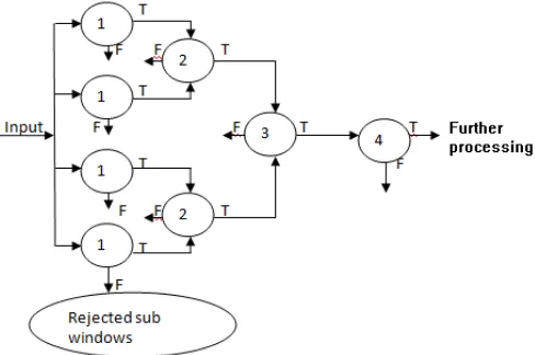
Available Online at www.ijpret.com 667 Simpler classifiers are used to reject the majority of subwindow, before more complex classifiers are called upon to achieve low false positive rates. The overall form of the detection process is that of a degenerate decision tree, what we call a “parallel cascade” (see Figure 6).
A series of classifiers are applied to every sub-window. The initial classifiers eliminates a large number of negative subwindows with very little processing. Layer first contain four classifier of same haar features. subwindows are forwarded in sequential manner i.e.,subwindow1,5,9 etc. to layer first node 1. Subsequent layers eliminate additional negatives but require additional computation. After few stages of processing the number of sub-windows has been reduced radically. Further processing can take any form such as additional stages of the cascade (as in our detection system) or an alternative detection system. A positive result from the first classifier triggers the evaluation of a second classifier which has also been adjusted to achieve very high detection rates. A positive result from the second classifier triggers a third classifier, and so on. A negative outcome at any point leads to the immediate rejection of the sub-window. To determine number of Haar-like feature we use the OpenCV Library [24].
Stages in the cascade are constructed by training classifiers using LDA and then adjusting the threshold to Minimize false negatives.
Figure 6: Proposed parallel cascade of classifier for face detection.
Available Online at www.ijpret.com 668 predicted bounding box and ground truth bounding box. Multiple detections of the same face in an image are considered false positive detections.
A. Time Complexity
Consider numbers of training samples are 𝑁 . For finding the optimal threshold of each feature
needs 𝑂(𝑁 log 𝑁)/𝑝. Assume that the size of the feature set is 𝑀 and the number of weak
classifiers to be selected is 𝑇. The time complexity for training PGSLDA classifier is
𝑂(𝑀𝑇𝑁 log𝑃𝑁
𝑃 ). The time complexity for GSLDA testing pass is 𝑂(
𝑁𝑀𝑇
𝑃 + 𝑀𝑇
3). 𝑂(𝑁)/𝑝 is time
complexity for finding mean and variance of each feature. 𝑂(𝑇2) is the time complexity for
calculating correlation for each feature. Since, we have features and the number of weak
classifiers to be selected is 𝑇, the total time complexity for PGSLDA is 𝑂(𝑁𝑀𝑇/𝑝 + 𝑀𝑇3).
Hence, the total time complexity is 𝑂(𝑀𝑇𝑁 log𝑃𝑁
𝑃 +
𝑁𝑀𝑇
𝑝 + 𝑀𝑇
3).
III. RESULT AND DISCUSSION
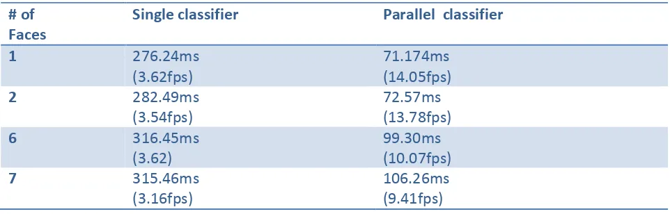
This section is organized as follows. The data sets used in this experiment, including how the performance is increased and ROC of face detection in figure 7. We tested our face detectors on the low resolution faces dataset, MIT+ CMU frontal face test set. The complete set contains 130 images with 507 frontal faces. In this experiment, we set the scaling factor to 1.2 and window shifting step to 1 pixel. Also it’s negative error rate is less as compare with GSLDA (shown in figure 8) [1]. Time required to detect face from given image is shown in Table I. From observation we can say image contain less number of faces required less time to process as compare to more number of face image.
TABLE I. PERFORMANCE OF PROPOSED FACE DETECTION SYSTEM WITH 640×480 RESOLUTION IMAGES
# of Faces
Single classifier Parallel classifier
1 276.24ms
(3.62fps)
71.174ms (14.05fps)
2 282.49ms
(3.54fps)
72.57ms (13.78fps)
6 316.45ms
(3.62)
99.30ms (10.07fps)
7 315.46ms
(3.16fps)
Available Online at www.ijpret.com 669
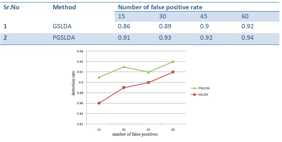
TABLE II. DETECTION RATE IN GSLDA AND PGSLDA METHOD.
Sr.No Method Number of false positive rate
15 30 45 60
1 GSLDA 0.86 0.89 0.9 0.92
2 PGSLDA 0.91 0.93 0.92 0.94
Figure 7: ROC curve for GSLDA and PGSLDA face detector on MIT+CMU test set.
Available Online at www.ijpret.com 670
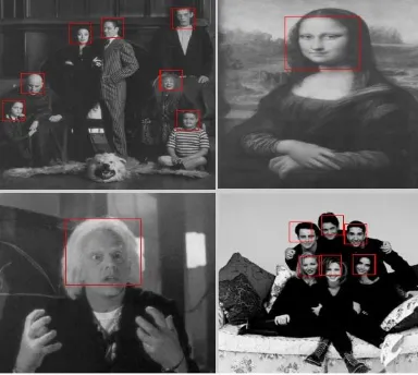
Figure 9. Output of face detector on number of test images from the MIT+CMU test set.
IV. CONCLUSION
In this work, Greedy Sparse Linear Discriminant Analysis (GSLDA) and Parallel GSLDA (PGSLDA) method for face detection had implemented. In GSLDA, we found that feature selection play a vital role in the overall performance of face detection. Face detection using GSLDA method is done in three steps: The step is preprocessing. In this step, input image is processed to get Integral Image which computes the Haar-like features quickly. Haar-like feature are used to detect the faces in given image. Experimental result had proven that Haar-like rectangle feature perform well on frontal images. The second step is feature extraction method. Linear Discriminant Analysis (LDA) method has used as feature extraction. LDA uses class-separability criterion. LDA also maintain the importance of imbalanced data sets. LDA selects maximum eigen value as threshold which discriminate face class from nonface class. LDA act as a weak classifier. The third step is to arrange LDA weak classifier in coarse-to-fine cascaded manner which is computationally efficient and gives high detection rate. Drawback of GSLDA is that first cascaded node must have to check each subimage. Frequently used stages are always busy so face detection time increased. GSLDA require much training time. GSLDA detection rate is 92%.
Available Online at www.ijpret.com 671 Parallel GSLDA based face detection technique is faster and computational efficient than GSLDA. PGSLDA with 41 Haar-like features required 8.33 second time for training.
Detection rate is directly proportional to the number of features in classifier. For good detection it should be in between 40-200. Haar-like feature increases complexity also increases. Proposed PGSLDA detect 14 frames per second on a standard system. Also we found that face detection rate is directly proportional to number of faces in that image. PGSLDA face detection has detection rate 94 % with false positive rate of 0.28 %. An approach that can optimally build a cascade classifier may be a future topic.
REFERENCES
1. C. Shen, S. Paisitkriangkrai, and J. Zhang,“ Efficiently learning a detection cascade with
sparse Eigenvectors,” IEEE Transaction on Image processing, vol.20, no.1, 2011.
2. E. Hjelmas and B. K. Low, “Face Detection: A Survey,” Computer Vision and Image
Understanding, vol. 83, pp. 236-274, 2001.
3. Monika Verma,”A Hybrid Approach to Human Face Detection,” International Journal of
Computer Applications (0975 – 8887), Volume 1 – No. 13,2010.
4. H.A. Rowley, S. Baluja, and T. Kanade,” Neural network-based face detection,” IEEE
Transaction on Pattern Analysis and Machine Intelligence, vol. 20,no.1, pp.23–38, 1998.
5. C. Garcia and M. Delakis,”Convolutional face finder: a neural architecture for fast and robust
face detection,” IEEE Transaction Pattern Analysis and Machine Intelligence, vol.26, no.11, pp.
1408–1423, 2004.
6. C. Papageorgiou, M. Oren, and T. Poggio, “A general framework for object detection,”
International Conference on Computer Vision, 1998.
7. P. Viola and M. Jones, ”Rapid object detection using a boosted cascade of simple features,”
Conference on Computer Vision and Pattern Recognition, 2001.
8. P. Viola and M. J. Jones, “Fast and robust classification using asymmetric AdaBoost
and a detector cascade,” Proc. Advance Neural Information Process System, Canada, pp. 1311–
1318, 2002.
9. P. Viola and M. J. Jones, “Robust real-time face detection,” International Journal Computer
Available Online at www.ijpret.com 672
10.B. Moghaddam, Y. Weiss, and S. Avidan, “Fast pixel/part selection with sparse
Eigenvectors,” Proc. IEEE International Conference on Computer Vision, Brazil, pp. 1–8, 2007.
11.L. Bourdev and J. Brandt, “Robust object detection via soft cascade,” Proc. IEEE Conference
Computer Vision & Pattern Recognition, San Diego, vol. 2, pp. 236–243, 2005.
12.R. O. Duda, P. E. Hart, and D.G. Stork, Pattern classify,2nd Edition,wiley-Interscience, 2000.
13.E. Hjelmas and B. K. Low, “Face Detection: A Survey,” Computer Vision and Image Understanding, vol. 83, pp. 236-274, 2001.
14.http://www.face-rec.org/algorithms.
15.H.A. Rowley, S. Baluja, and T. Kanade,” Neural network-based face detection,” IEEE
Transaction on Pattern Analysis and Machine Intelligence, vol. 20,no.1, pp.23–38, 1998.
16.J. Sochman and J. Matas and Waldboost,”learning for time constrained sequential
Detection,” Conference on Computer Vision and Pattern Recognition, vol.2, pp 150–157, 2005.
17.M. T. Pham and T. J. Cham, “Fast training and selection of Haar features using statistics in
boosting-based face detection,” IEEE International Conference Computer Vision, Brazil, pp. 1–7,
2007.
18.S. Romdhani, P. Torr, B. Scholkopf, and A. Blake, “Computationally efficient face detection,”
in Proc. IEEE International Conference Computer Vision, Canada, pp. 695–700, 2001.
19.S. Balakrishnama, A. Ganapathiraju,” LDA -A brief tutorial,”2007.
20.P.J. Philips, P.J. Grother, R.J. Micheals, “Face recognition vendor test: Evaluation report,”
National Institute of Standards and Technology, 2003.
21.R. Kleihorst, M. Reuvers, B. Krose, and H. Broers, “A smart camera for face recognition,”
Proceedings of the IEEE International Conference on Image Processing, pages 24–27, 2004.
22.A. Lanitis, C.J. Taylor, and T.F. Cootes,”Toward automatic simulation of aging effects on face
images,” IEEE Transactions on Pattern Analysis and Machine Intelligence, vol.24, no.4, pp.442–
455, 2002.
Available Online at www.ijpret.com 673
24.Fei Zuo,”Embedded face recognition using cascaded structures,” Eindhoven Technical
Universities Eindhoven, 2006.
25.Ander Jorgensen,”AdaBoost and Histograms for Fast Face Detection,” ISSN-1653-5715, URL:
www.csc.kth.se, 2006.
26.Andrew King,” A Survey of Methods for Face Detection,” 992 550 627, March 3, 2003.
27.Monika Verma,” A Hybrid Approach to Human Face Detection,” International Journal of
Computer Applications (0975 – 8887), Volume 1 – No. 13,2010.
28.ORL Database available at http://cvc.ORL.edu/
![Figure 3. Haar wavelet frameworks [5].](https://thumb-us.123doks.com/thumbv2/123dok_us/8728827.1745906/6.612.206.408.214.333/figure-haar-wavelet-frameworks.webp)