A THEORETICAL ESTIMATION OF CURRENT DENSITY J AND ORDER PARAMETER ? FOR THIN SUPERCONDUCTOR USING MICROSCOPIC THEORY OF RESISTIVE STATE

Available Online at www.ijpret.com 75

INTERNATIONAL JOURNAL OF PURE AND

APPLIED RESEARCH IN ENGINEERING AND

TECHNOLOGY

A PATH FOR HORIZING YOUR INNOVATIVE WORK

A THEORETICAL ESTIMATION OF CURRENT DENSITY J AND ORDER PARAMETER ∆

FOR THIN SUPERCONDUCTOR USING MICROSCOPIC THEORY OF RESISTIVE

STATE

VIJAY KUMAR VERMA

Associate Professor, Department of Physics, Gaya College, Gaya—823001. (Bihar)

Accepted Date: 06/01/2015; Published Date: 01/02/2015

\

Abstract: Using the microscopic theory of resistive state in which the velocity of the superconducting condensate increases under the action of the electric field, the current j and order parameter ∆ for thin superconductor were evaluated. The obtained theoretical results are in good agreement with theoretical workers.

Keywords: Phase-slip centre (PCS), superconducting condensate , Josephson Frequency, gapless superconductivity, TDGL (Time –dependent Ginzburg-Landau) equation, Current-Current state, Electric field penetration depth, resistive state, super current oscillations.

Corresponding Author: MR. VIJAY KUMAR VERMA

Access Online On:

www.ijpret.com

How to Cite This Article:

Vijay Kumar Verma, IJPRET, 2015; Volume 3 (6): 75-84

Available Online at www.ijpret.com 76

INTRODUCTION

The fluctuation mechanism of phase-Slip Centre (PCS) formation role only in a very narrow vicinity of TC. . If one goes beyond the special interval the probability of fluctuation becomes

extremely small. Moreover, if the current through the sample is sufficiently small there will be no mechanisms of formation of PSC and the voltage across the channel will be zero and the sample will be in a purely superconducting state .When the current exceeds some limiting value (dependent on sample length)the condition of attraction to spontaneous formation of PSC are satisfied (the system falls in the region of attraction to the limiting cycle) and one PSC appears in sample. This finds its reflection as voltage step in the I-V characteristic. When the currents is increased further, two there are more PSCs, may appear in the sample, this accompanied by corresponding voltage steps in the I-V characteristics. This the case in samples of finite length. In an infinitely long sample, the total number of PSCs is always large and its density increases smoothly with the current, the corresponding I-V characteristics has the form of a smooth curve.

The qualitative picture of formation of a PSC consists in that the velocity of the superconducting condensate increases under the action of the electric field. Then at some time and at some place in the sample the velocity reaches such a value (not unstable and the order parameter) falls to zero at this place. When ∆ turn to zero the phase coherence is destroyed. Then the formation of the superconducting condensate starts again in the vicinity of this point since the

sample has a temperature below . Superconducting is restored, superconducting regions to

the right and to the left from the PSC is changed by 2 as compared to the phase difference in the initial state

MATERIALS AND METHODS: Reiger, et al.1 [1], proposed a numerical model for the PSC formation. They defined the moment of PSC formation as that when the free energy of the sample section, increasing due to the acceleration of the Cooper pairs by the electric field , becomes higher than the free energy of the state which this section would have if the phase difference between its ends were 2 less. This condition is, of course, quite artificial and the model proposed by Reiget, et al.[2] , is useful only as the first step in solving the problem of the resistive state.

One discuss now the qualitative picture of formation of the voltage across the PSC: one follow here the model suggested by Skocpol et al.[2], (SBT-model).

The total current density can be represented as a sum of the supercurrent jS and the normal

Available Online at www.ijpret.com 77

1

n s s

Q

j E j j

c t           _  _  

  _{--- (1)}

All the quantities in the right-hand side of equation (1) depend on time varying periodically with the period to=2 / j where j is the Josephson frequency. We are interested in the

time-averaged voltage which is measured experimentally. After averaging equation over time the term = vanishes due to periodically and one has

J=-

+ js ……... (2)

In the SBT-model, the equation for the time- averaged potential ф is written simply in the form

2 2 2 1 E I    _   --- (3) Where IE is considered to be independent of x. The solution of equation (3) in then

1 sinh E x x c I    --- (4)

Where c is a constant and x1 is the point where = 0.We assume for simplicity that the ends of

the superconducting channel are connected with the bulk superconducting ‘bank’ which are in

equilibrium so that x=x1 corresponds to the left end of the channel. One obtained equation

 

_cosh 1

x

c E

x x

j j x c

I I

 

 

Let us suppose that the sample has a finite length and there is only one PSC in it at the point x=x0. Then the constant c is

 



0 01



cosh

x E

E

j j x I

c

x x I 

  



The potential difference between the left end of the channel x=x1 and the PSC is

 





0 1

1 0 tanh

E x

E

x x

I

j j x

I 

    

This is the potential just to the left from the PSC. If one considers now the other (right) end of the channel, x=x2 ,where one assumes also ф=0 then one obtains for the potentialф2 just to the

right from the PSC

 





2 0

2 0 tanh

E x

E

x x

I

j j x

I 

    

Available Online at www.ijpret.com 78

 





0 1 2 0

2 1 0 tanh tanh

E

x

E E

x x x x

I

j j x

I I





   

       _  _

  _{--- (5)}

at point of the PSC. The potential jump across the PSC, is due to the phase-slip process. Indeed, if we average the difference ф(x0+1) ф(xn+0) over time then

































0 0 0 0 0 0 0 0 0 0 0 0 0 0 0 0 0 0 0 0 0 1 1 0 0 2 2 0 0 1 1 2 2 t t t x x x x I

dt x x

I e t e t

x x

I

dt

I e dt t et t

                     _   _{ }    _                 _  _    







Here  _{is the phase difference between two points just to the right and to the left of the PSC.}

We use here the continuity of the potential ф at the PSC. As was solid above the phase 

change 2 by during the phase-slippage, so the last expression is 2 /2et0= / 2e where is the

Josephson frequency.

The time-averaged pair chemical potential p= ( z / ) is constant in regions from x1 to x0 and

from x0 to x2. Indeed, the time-average electric field.

RESULTS OF THE NUMERICAL SOLUTION OF TIME-DEPENDENT SUPERCONDUCTIVITY EQUATION:

One has said that the phase slip process have essentially non-linear nature so it is very difficult obtain the mathematically exact analytical solution even for the comparatively simple-dependent equations and such a solution is not yet found. Numerical methods of solving these equations can be very helpful here.

The first results in this line have obtained by Kramer and Barat off [5]. They investigated the TDGL equations which are valid in the case of gapless superconductivity. In this corresponds to the limit I-- I ,when the lack of a gap in the energy spectrum is due to a strong electron phonon interaction





2

2

2 1 0

u i t x         _  _      

  _{--- (6)}

* 1 * 2 j x i               _  _

Available Online at www.ijpret.com 79 Similar equation apply for gapless superconductors with large concentration of magnetic

impurities (Gor, kov and Eliashberg[6]), where one has to put u =12. Kramer and Barat off [5] solved equation (1) and (2) with two values of the parameter u = 5.79 ,

and u=12 have obtained the following results

1. When the current js less than some value jmin (jmin = 0.326) for u =5.79 and jmin = 0.28 4 for u

= 12 perturbation with respect to the purely superconducting state decay and the superconductor returns to the uniform current-carrying state with the order parameter. Note that in this case jmin < jc where jc =2/2 is the Ginsburg –Landau critical current.

2. When the current is larger than the other threshold value j2 , where j2 =0.335 for u=5.79 and

j2 =0.291 for u=12 the superconducting current carrying state disappear .Thus, when j>j2 the

superconducting state appears to be unstable . The threshold current j2 coincides with the

stability limit of the normal superconducting interface studied by Likharev [7] and Likharev and Yokobson [8].

Within the interval between jmin and j2 there exist the solution which corresponds to

phase-slippage. This solution behaves as follows. The channel remains superconducting over almost all its length , but at at some point local oscillations of the order parameter ∆ take place. When ∆ becomes zero its phase experience a jump by 2 . When the current approach jmin the

oscillation period tends to i infinity and the solution transforms into the Langer and Ambegaokar solution [9] of equation asymptotically as t the amplitude of oscillations decreases with the increase in the current. The Kramer and Barat off [5] solution for u=5.79 and j=jmin .

These results were the first direct verification of the existence of the solution with phase slippage and given evidence of the existence of the limiting cycle with oscillations of the type required for the system described by equations (6) and (7).

Equations (6) and (7) were investigate more recently also by lelev,et al. They use the gapless equations for modelling the processes in superconductors with a gap in the energy spectrum. The main idea was as follows. When there is the gap (i.e., when Γ ) the electron field penetration depth is large _{. This situation can be simulated in terms of}

equations (6) and (7) by giving a small value to the parameter u: since IE in equation (2) is

proportional to

1 2 u



this will ensure IE >>1 Therefore, by means of the simplest TDGL

Available Online at www.ijpret.com 80 The numerical results described above are of great importance. They prove first of all the very fact of the existence of the solutions which corresponds to phase slippage and verify thereby our general understanding of the nature of the resistive state. The numerical methods, however, cannot give the complete information of the resistive state properties and how they depend on various parameters of the sample and on conditions of the real experiment. [11-13].

The Microscopic Theory of The Resistive State: One turn now the more sophisticated theory of the resistive state based on the microscopic dynamic theory of superconductivity.

One consider below the time-dependent equations in the most interesting case, from both the experimental theoretical point of view, when there is a gap in the energy spectrum of the

superconductor, which corresponds to temperatures



_{c ph}



2 1 .

c

T T

T

  .we recall that

the electric field penetration depth is large in large in this case: I

1 2 _1.

E

I   

The following analysis will be based on the results of Ivlev et.al., [10] and Kippin. [14]. When one can write equation TDGL in the form

 

2 2

1 1

Q

j Q Q

t u z z

    

   _    _

      _{……….. (8)}

The estimation of the first term in the right hand side of equation (8) gives

1

1 2

0

Qt  Q  _{. Where}

Q

– is the oscillating part of Q Q: Q| and the bar indicates the averaging core time. The

second and third terms are of the Q at distances of order Q Q so the Q-Q. The oscillating part

Q

– will be of the same order as Q only at shorter distance from a PSC.

So one can obtain the following results:

1. The phase slip region has the size of order of ( )T  .Here all the variables oscillate strongly. At the moments when  0 the phase Z experiences jumps by 2 and  (x 0)

goes to infinity. The amplitude to oscillations is of order GL  _.

2. As one goes away from of PSC oscillations in  becomes practically independent of time at distance x x2 

 

T T .Here    where  is equal to

.The order

Available Online at www.ijpret.com 81 3. At distances

1 2

(I_E)  x L _{oscillations of all the quantities are negligible. Here the}

relaxation of

1

6 _{p n}

e  

 

 _  _

  _{takes place .The imbalance is created in the PSC region as a}

result of phase slips. As the potential  and the normal current jn ( x)

   _

decreases, the

supercurrent js _{increases and}  _{diminishes. The supercurrent} js_{reaches its maximum at the} midpoint between the PSCs.

Now one estimates the temperature range of validity of those results. The Josephson frequency

of oscillations j _{has the order of} 1



 _{.Since our equations are valid if}  1 _and

1

j ph

 _

one has the to see the temperature from the interval.

6

2 5

( _{c ph}) 1 ( _{c ph})

c

T _T

T

 _  

   

……… (9)

RESULTS AND DISCUSSIONS:

In this paper, we have studied and evaluated I-V characteristic current for thin superconductors from microscopic theory of resistive state. If the current through the sample is sufficiently small then there will be no mechanism of formation of phase slip centres (PSC) and the voltage across the channel will be zero and the sample is in the superconducting state .When the current exceeds some limiting values depending upon the sample length the conditions of spontaneous formation of PSC are satisfied .When one PSC appears this find it reflecting as the voltage step in the I-V characteristics. When the current is increased further two more PSC may appear and this is accompanied by corresponding voltage steps in the I-V characteristic. This is the case in samples of finite length. In an infinitely long sample the total number of PSC is always large and its density increases smoothly with the current and the corresponding I-V characteristics has the form of smooth curve. It is clear from the above discussion that the non-linearity of the system play the main role in the resistive state. The qualitative picture of formation of PSC consists in that the velocity of the superconducting condensate increases under the action of electric field. Then at some time and at the same place in the sample the velocity reaches such a value (not necessarily equal to the critical velocity ) that the superconducting state becomes unstable and the order parameter falls to zero at this place. When  turns to zero the phase coherence is destroyed . {16-18] Then the formation of the superconducting condensate state

Available Online at www.ijpret.com 82 as compared to phase difference in the initial state . As the phase slip process is non-linear one so it is very difficult to obtain the mathematically exact analytical solution for the simple time dependent equation. Numerical method have been employed to solve these equations. The results of three equations give direct verification of the existence of the phase slippage . It was found that the range of currents when the solution with phase-slippage exists is board and will

decrease value of  .This cannot J2 _{is proportion of} 1 _{of small}  _{. We have evaluated the}

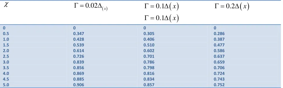
value of  as a factor of x for fixed values of  . The results are shown in Table T1 _.Our

results indicated the x decrease

 

x increases for fixed value of  . The values of 

 

x is larger for  0.02 and small for 0.2 . We have also studied the current voltage character

by using the dynamic theory of resistive state. We have taken three difference solution of 0

and a when 0 _{is a free parameter with} j ac _{is length of weak lin and} a. _{Our theoretical}

results indicates that for all the three given set of 0 _{and a, the current j increases with E}

linearly for higher values of E obeying ohm’s law .For the lower values of E there is slight departure from ohm’s law. In this region the order parameter and the superconductor are practically time independent and become of the highly non-adiabation behaviour of the order parameter and the superconductivity. When the frequency of oscillation is very high [19-35]

CONCLUSION:

In this paper using microscopic theory of resistive state, I have evaluated the value of current j

by taking different value of 0 _{and a.} 0 is free parameter and a is the length of weak links.

Here a is taken less than the coherence length (a ). Our theoretical result shows that for the

given set of 0 _{and a, current j increase with electric field E linearly and for high field E obeys}

Ohm’s law. For lower value of E, there is slight departure from Ohm’s law. . We have also

observed that the order parameter  coordinate dependence.

TableT1_{: The I-V characteristic calculated with difference} 0 _{We have taken values of}

 

0

 

0

 

0

2

, 0 0.9, 0.61 0.975, 0.35

3

i   a ii   a iii   a

(a is the length of weak link)

E

Value of j

0 2

, 0.68

3 a

  

0 0.975,a 0.35

  

0 0.9,a 0.61

    0 0.975,a0.35

Available Online at www.ijpret.com 83 0.10 0.15 0.20 0.25 0.30 0.35 0.40 0.45 0.50 0.55 0.60 0.478 0.496 0.523 0.558 0.572 0.576 0.632 0.659 0.671 0.696 0.734 0.426 0.443 0.472 0.518 0.518 0.532 0.559 0.577 0.596 0.624 0.656 0.405 0.421 0.476 0.473 0.492 0.511 0.535 0.556 0.578 0.599 0.612

Table T2: The coordinate dependence of order parameter  for different values of parameter

 _. 

 

0.02 _x

    0.1

 

x

 

0.1 x   

 

0.2 x    0 0.5 1.0 1.5 2.0 2.5 3.0 3.5 4.0 4.5 5.0 0 0.347 0.428 0.539 0.614 0.726 0.839 0.856 0.869 0.885 0.906 0 0.305 0.406 0.510 0.602 0.701 0.786 0.798 0.816 0.834 0.857 0 0.286 0.387 0.477 0.586 0.637 0.659 0.706 0.724 0.743 0.752 REFERENCES:

1. T.J.Rieger,D.J.Scalapino,and J.E. Merereau, Phy.Rev.,B6.1734 (1972).

2. W.J.Skocpol,M.R.Beasley and M.Tinkham.J.Low Tem.Phy.,16,145 (1974).

3. G.J.Dolan andL.D.Jackel.Phys.Rev.,39,1628 (1977).

4. M.J.Tinkhan,LowTemp.Phrs.,35,147 (1979).

5. L.Kramer and R.J.Watts.Tobin,Rev.Lett.,40,1041(1979).

6. G.M.Eliashberg,26,eksp.teor.Fiz.,61,1254 (1971)

7. K.K.Likharev,Pisma Zh. eksp tor Fiz.,20.730(1974).

8. K.K.Likharev and L.A.Yakosbon,Zh.eksp, tor Fiz.,68, 1150(1975).

9. R.A.Golus,Zh.eksp teor,Fiz.,71.347 (1976).

Available Online at www.ijpret.com 84

11.B.I.Ivlev,and N.B Kophinand, I.A. Larkin,J. Low Temp.Phys.,53,153(1983).

12.F.B.,Iviev Kophin,N.B.and C.J. Pethick,J. Low Temp. Phys.,41,297(1980).

13.R.J., Watts,Tobin, Krahanbuch, Y. and L.Kraker, J.Low Temp. Phys.,42 459(1983).

14.V.P., Galaiko, Zh eksp. Teor. Fiz.,66 379 (1974).

15.V.P., Galaiko, J.Low Temp. Phys., 26 483 (1977).

16.V.P. Galaiko,and V.M.Dmitriev, Fiz Mizh. Temp., 2, 199 (1976).

17.V.P. Galaiko, and M. Schumeiko,J. Low Temp. Phys.,27, 222 (1978).

18.M.J., Fink, Phys. Stat sol.(b),60, 843 (1973).

19.H.J., Fink, Phys. Lett. A.,42, 465(1973).

20.H.J. Fink, and R.S. Polsen, Phys. State sol. (b), 63, 317 (1974).

21.H.J. Fink, and R.S. Polsen, Phys. State sol. (b), 64, 20 (1975).

22.H.J. Fink, and R.S. Polsen, Phys. Rev. Let., 32, 762 (1975).

23.S.N., Artememno, Volkov, A.F. and A.F. and A.V. Zaitse, Pisma Zh. eskp, teor. Fiz., 28, 637 (1978).

24.J.R. Tucker, and B.I. Halperien, Phys. Rev., B. 68 102 (1992).

25.H., suehiro, Awa, K. and H. Yasuhava, sol. Stat. commun., 67, 1641 (1994).

26.M.S. Dressehans, and G. Riganux, Adv. Phs.,50, 139 (1980).

27.D.J.W., Geldart, can J. Phys.,65, 3139 (1996).

28.Q.J. Chen and I. Kosztin, Phy.Rev.B 63, 184519 (2001).

29.Q.J. Chen and J.R. Schrieffer , Phys. Rev. B 66, 014512 (2002).

30.H. Heiselberg, Phys. Rev. Lett (phy) 93,040402(2004).

31.J.Stajic,Q.J.Chen and K.Leven , Phys.Rev. Lett.(Phy)94 ,060401(2005).

32.M.Jaslon,H.Buljan and M.Solijacic,Phys .Rev. B 80 ,245235(2009).

33.M. J. Balaber,M.D.Arnold and M.J. Ford, J.Phys. Codence Matter.22 096601(2010).

34.A. Vakil and N.Enghita , Science 332, 1291(2011).