The Thirty-Third AAAI Conference on Artificial Intelligence (AAAI-19)
CircConv: A Structured Convolution with Low Complexity
Siyu Liao, Bo Yuan
Department of Electrical and Computer Engineering, Rutgers University [email protected], [email protected]
Abstract
Deep neural networks (DNNs), especially deep convolutional neural networks (CNNs), have emerged as the powerful tech-nique in various machine learning applications. However, the large model sizes of DNNs yield high demands on computa-tion resource and weight storage, thereby limiting the prac-tical deployment of DNNs. To overcome these limitations, this paper proposes to impose the circulant structure to the construction of convolutional layers, and hence leads to cir-culant convolutional layers (CircConvs) and circir-culant CNNs. The circulant structure and models can be either trained from scratch or re-trained from a pre-trained non-circulant model, thereby making it very flexible for different training environ-ments. Through extensive experiments, such strong structuimposing approach is proved to be able to substantially re-duce the number of parameters of convolutional layers and enable significant saving of computational cost by using fast multiplication of the circulant tensor.
Introduction
Large-scale deep neural networks (DNNs), especially deep convolutional neural networks (CNNs), have achieved ex-traordinary success in various artificial intelligence appli-cations such as image recognition, video analysis, etc. (Krizhevsky, Sutskever, and Hinton 2012; He et al. 2016; Karpathy et al. 2014). However, the large model sizes of DNNs make themselves both computation-intensive and memory-intensive, thereby potentially hindering the ex-pected widespread deployment of DNNs in many latency-sensitive resource-constrained applications.
To address these limitations, many approaches (Han, Mao, and Dally 2015; Gong et al. 2014; Wen et al. 2016; Feng and Darrell 2015) have been proposed to reduce the computational cost and/or memory footprint of DNNs. In general, those existing efforts can be roughly categorized as two types: fully-connected layer-oriented reduction, such as connection pruning (Han, Mao, and Dally 2015)1, weight clustering (Gong et al. 2014), and convolutional layer-oriented reduction, such as low rank approximation (Jader-berg, Vedaldi, and Zisserman 2014), sparsity regularization
Copyright c2019, Association for the Advancement of Artificial Intelligence (www.aaai.org). All rights reserved.
1
It can also bring reduction for convolutional layers to some degree. But the most reduction in the number of parameters is achieved on fully-connected layers.
(Wen et al. 2016; Feng and Darrell 2015). Nowadays, con-sider 1) convolutional layers consume most of the com-putational processing in DNNs and 2) many state-of-the-art DNNs, such as ResNet (He et al. 2016) and Inception (Szegedy et al. 2015), use very few fully-connected layers that only contain a small portion of parameters of the en-tire models (e.g. less than 5%parameters for fully-connected layers in ResNet-152), the reduction on computational cost and numbers of parameters of convolutional layers become very essential.
Technical preview and advantages. In this paper we propose to impose the circulant structure to the construc-tion of convoluconstruc-tional layers shown in Figure 1, yielding low-computation-complexity, low-space-costcirculant con-volutional layers (CircConvs)and the corresponding circu-lant CNNs. Different from prior convolutional layer-oriented compression approaches that are based on the unstructured tensors, the model-size reduction in this paper results from the use ofcirculant tensors(Rezghi and Eld´en 2011): The weight tensors for convolutional layers, which were origi-nal unstructured, are now constructed in the circulant for-mat, thereby leading to substantial reduction in computa-tional cost and numbers of parameters. In short, the proposed approach brings the following advantages:
1) It reduces the space cost of the convolutional layers because of the inherent spatial regularity of circulant tensors, thereby resulting in high compression ratios for the overall network model sizes.
2) It saves the computation of the convolutional layers by leveraging the fast circulant tensor-specific multiplication algorithm, and hence greatly reduces the computational cost of the entire networks.
3) It enables the improved accuracy for the correspond-ing circulant CNNs as compared with the similar-size non-circulant CNNs. In other words, the benefits of model-size reduction resulting from using circulant convolutional layers can translate to the increase of accuracy.
4)The circulant structure can be imposed by either train-ing from scratch or re-traintrain-ing from a pre-trained non-circulant model, thereby making non-circulant CNNs very flexi-ble for different training environments.
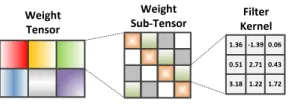
Figure 1: Illustration of a circulant weight tensor. Blocks of the same color in the middle share the same set of kernel weights (on the right). This significantly reduces the total amount of parameters needed to represent this tensor. In ad-dition, the placement of blocks displays a circulant structure, facilitating FFT-based fast algorithms.
and floating point operations (FLOPs) with negligible ac-curacy drop. In addition, the experiments on wide ResNets show that the proposed approach leads to better accuracy than the non-circulant ResNet models with similar numbers of parameters. Furthermore, we also compare the FLOPs of the proposed circulant CNN models with the non-circulant CNN models, and experimental results show that our pro-posed method can reduce FLOPs for the inference.
Related Work
Weight pruning/clustering. (Gong et al. 2014) proposes to cluster the weights to reduce the model sizes of DNNs. In that work, various types of weight clustering, including scalar quantization, product quantization, residual quantiza-tion, are investigated. (Han, Mao, and Dally 2015) proposes a multi-step compression pipeline comprising of weight pruning, clustering, and quantization to achieve high com-pression ratios for the entire networks. Notice that as indi-cated in (Wen et al. 2016), because most parameter reduc-tion in (Gong et al. 2014) and (Han, Mao, and Dally 2015) are achieved on fully-connected layers, the reduction in the computational cost of convolutional layers is not significant. In addition, it is also found that weight parameters in fre-quency domain can be pruned (Wang et al. 2016) or clus-tered via a hashing function (Chen et al. 2016).
Low rank approximation (LRA). LRA is an efficient approach to compress DNNs (Jaderberg, Vedaldi, and Zis-serman 2014; Sainath et al. 2013; Zhao, Li, and Gong 2016). In (Jaderberg, Vedaldi, and Zisserman 2014), various types of LRA-based solutions are proposed to reduce the numbers of parameters and computational cost of convolutional lay-ers. However, the model-size reduction using LRA usually requires costly reiterations of decomposition and fine-tuning to minimize the approximation error and retain the accuracy. Sparsity regularization.Increasing the sparsity of net-work by performing regularization is another popular tech-nique to reduce model sizes of DNNs. (Feng and Darrell 2015), (Girosi, Jones, and Poggio 1995) and (Wen et al. 2016) propose several sparsity-introducing techniques by leveraging different types of regularization, such as L1-norm, group-lasso etc. Though sparsity regularization essen-tially provides a stable reduction in computational cost, the resulting reduction in model size is not significant.
Structured transform.By using structured matrices, the structured transform can enable very high compression
ra-tios for fully-connected (FC) layers. In (Sindhwani, Sainath, and Kumar 2015; Cheng et al. 2015; Moczulski et al. 2015), weight matrices are constructed in the format of structured matrices to achieve significant reduction in model sizes. (Zhao et al. 2017) further proves that the low displacement rank-based neural networks, which are the generalization of the structured networks can still exhibit universal approxi-mation property. However, the FC layer-specific approaches in (Sindhwani, Sainath, and Kumar 2015; Cheng et al. 2015; Moczulski et al. 2015) cannot be directly applied to the popular and important convolutional layers. Instead, con-sider FC layer can be viewed as a type of special convo-lutional layer, our proposed circulant convolution-imposing approach has more generality and is very useful for practi-cal applications. Particularly, compared with (Cheng et al. 2015) and (Sindhwani, Sainath, and Kumar 2015), we gen-eralize the structure from regular 2D weight matrix in fully connected layer to the 4D weight tensor in convolutional layer, where the underlying computation is totally different. Moreover, this paper is significantly different from two related works (Ding et al. 2017; Wang et al. 2018) in fol-lowing aspects: 1) we propose an approach on direct opera-tion on 4D circulant tensor with all the algorithm-level de-tails; while prior works require extra processing step to con-vert tensor to matrix; 2) we perform comprehensive experi-ments on circulant convolution and present accuracy results and analysis on different datasets; 3) we propose a novel al-gorithm to convert non-circulant tensor into circulant ten-sor, thereby making obtaining circulant convolution on pre-trained non-circulant models become possible; while prior works can only train the structure from scratch.
Imposing Circulant Structure to
Convolutional Layers
Circulant Convolutional Layer
Conventional convolutional layer. In general, a convo-lutional layer maps a 3-dimensional input tensor X ∈
RW0×H0×C0 into a 3-dimensional output tensor Y ∈ RW2×H2×C2through convolution with a 4-dimensional
ker-nel tensor W ∈ RW1×H1×C0×C2. Here W
i and Hi for
i = 0,1,2, are the spatial width and height of the input, kernel, and output tensor, respectively;C0 andC2 are the
number of input channels and output channels. The convo-lution operation is expressed as follows:
Y(w2, h2, c2) = W1
X
w1=1 H1
X
h1=1 C0
X
c0=1
X(w2−w1, h2−h1,
c0)· W(w1, h1, c0, c2)
. (1)
Y(w2, h2,:) = W1
X
w1=1 H1
X
h1=1
X(w2−w1, h2−h1,:)
∗ W(w1, h1,:,:)
, (2)
where∗ and:denote the matrix-vector multiplication and the range of indices, respectively.
Circulant convolutional layer.Different from a conven-tional convoluconven-tional layer, the circulant convoluconven-tional layer has a weight tensorW that exhibits circulant structure. In other words, theWof a circulant convolution layer is a 4D
circulant tensors(Rezghi and Eld´en 2011). In general, a cir-culant tensor can exhibit circir-culant structure along any pair of its dimensions. However, asW1andH1are usually much
smaller thanC0 andC2 for tensorW, we impose the
cir-culant structure along the input channel and output channel dimensions to achieve high model-size compression ratio. Note that in practice we need to partition the tensorWinto circulant sub-tensors of sizeW1×H1×N×N. This is
nec-essary because the circulant structure requires that the two corresponding dimension must be equal, whileC0 andC2
are usually not the same. LargerN means larger compres-sion ratio but it could hurt the model performance to some degree. By adjusting the partition sizeNwe can balance the trade-off between compression ratio and model accuracy.
More specifically, letN be the partition size withC0 =
R×N andC2 = S ×N 2, thenW can be defined by a
4-dimensional base tensorW0∈
RW1×H1×RN×S:
W(w1, h1, c0, c2) =W0(w1, h1, p, q), (3)
where p, q are indices satisfying bc0/Nc = bp/Nc, bc2/Nc=q, andc0−c2 ≡p (modN). Fig. 1 illustrates
the circulant structure of weight tensorW. From this fig-ure, it can be seen that the circulant structure is imposed to
W along the input/output channel dimensions. The block-circulant weight tensor consists of six block-circulant weight sub-tensors, where different colors represent different circulant weight sub-tensors. Each circulant weight sub-tensor con-sists of sixteen kernel filters that are represented in different colors such as green and yellow.
Fast Forward and Backward Propagation Schemes
on Circulant Convolutional Layer
Eq. 3 shows that the weight tensorWof a circulant convo-lutional layer exhibits the circulant structure and has the re-duced number of independent parameters. Besides, accord-ing to the tensor theory (Rezghi and Eld´en 2011), circulant tensor also has the advantage of fast multiplication. Since multiplication is the kernel computation in neural network training and inference, the existence of fast multiplication of circulant tensor enables the immediate reduction in compu-tational cost. Next, we describe the fast forward and back-ward propagation schemes by leveraging the fast multiplica-tion of circulant weight tensor.
2
Zero-padding is needed whenNdoes not divideC0orC2.
Fast forward propagation.We first present the fast for-ward propagation scheme. Recall that Eq. 2 is the forfor-ward propagation scheme for a general convolutional layer. To ease the notation, defineNk = ((k−1)N+ 1, ..., kN)for
k= 1, ...,max(R, S), and rewrite Eq. 2 as below:
Y(w2, h2, Ni) = W1
X
w1=1 H1
X
h1=1 R
X
j=1
X(w2−w1,
h2−h1, Nj)∗ W(w1, h1, Nj, Ni)
, (4)
where i ∈ {1, . . . , S}. According to (Rezghi and Eld´en 2011; Pan 2012), Fast Fourier Transform (FFT) can be used to accelerate the multiplication of a fiber and a slice of cir-culant tensor with time complexity reduced fromO(N2)to
O(NlogN). Therefore, whenWis a circulant tensor, Eq. 4 can be reformulated using FFT as below:
Y(w2, h2, Ni) = ifft
XW1
w1=1 H1
X
h1=1 R
X
j=1
fft X(w2−w1,
h2−h1, Nj)
◦fft W0(w1, h1, Nj, Ni)
. (5)
Here◦is the element-wise multiplication.
Fast backward propagation. Now consider backward propagation. Given loss function L, it is well known that the goal of backpropgation algorithm (LeCun et al. 1998) is to compute gradients of loss functionLwith respect to each weight and input. Hence according to the chain rule, the gra-dient computation for circulant convolutional layer can be derived from Eq. 3 and Eq. 4 as below:
∂L ∂W0(w
1, h1, p, q) =
W2
X
w2=1 H2
X
h2=1 qN
X
c2=(q−1)N+1
∂L ∂Y(w2, h2, c2)
∂Y(w2, h2, c2)
∂W0(w
1, h1, p, q)
, (6)
∂L ∂X(x, y, c0) =
W1
X
w1=1 H1
X
h1=1
X
c2≡c0(modN)
∂L
∂Y(w1+x, h1+y, c2)
∂Y(w1+x, h1+y, c2)
∂X(x, y, c0) . (7)
Again, according to (Rezghi and Eld´en 2011), whenWis a circulant tensor, Eq. 6 and Eq. 7 can also be accelerated by using FFT as below:
∂L ∂W0(w
1, h1, Nj, i) =ifft(
W2
X
w2=1 H2
X
h2=1
fft( ∂L
∂Y(w2, h2, Ni)
∂L ∂X(x, y, Nj)
=ifft( W1
X
w1=1 H1
X
h1=1 S
X
i=1
fft(
∂L
∂Y(w1+x, h1+y, Ni)
)◦fft(wj0,i)), (9)
wherex0
jandw0j,iare fibersX(w1, h1, T)andW0(x, y,(j− 1)N+T, i)withT = (1, N, ...,2).
Capability of training Circulant CNN from scratch.It should be noted that the gradient computations described in Eq. 8 and Eq. 9 are actually based onW0. Since we can
al-ways construct the circulant tensorWfrom base tensorW0
using Eq. 3, Eq. 8 and 9 imply that the circulant structure of weight tensorW is always kept during the training phase. In other words, if we initialize W as the circulant tensor at the initialization stage of training, then during the train-ing procedure Eq. 8 and 9 can guaranteeW always exhibit circulant structure. Therefore, a circulant CNN can be com-pletely trained from the scratch.
Conversion from Non-circulant Tensor to
Circulant Tensor
Forward and backward propagation section indicates that a circulant convolutional layer can be trained from scratch. In this subsection, we also present a conversion technique that can directly convert a non-circulant weight tensor to a circu-lant one. Such conversion is very useful when a pre-trained model is already available and needs to be imposed with cir-culant structure.
Specifically, the proposed conversion technique is based on the circulant approximation approach (Chu and Plem-mons 2003) used for circulant matrix. In matrix theory, let
Z1∈RN×N denote a permutation matrix as following:
Z1=
0 1 0 . . . 0
0 0 1 . . . 0
..
. . .. . .. ...
0 1
1 0 0 . . . 0
. (10)
Then a circulant matrixWcirc ∈ RN×N with its first row
w= (w0, w1, . . . , wN−1)can be represented in the
polyno-mial form ofZ1as follows:
Wcirc=P
N−1
i=0 wiZ1i. (11)
According to (Chu and Plemmons 2003), for a non-circulant matrixWnon−circ ∈RN×N, its nearest circulant
matrixWcirc(measured in the Frobenius norm) is given by
projection:
w=projNWnon−circ,
∀wi∈w, wi= 1
NhWnon−circ,Z1
i
iF,
(12)
whereh·,·iFis the Frobenius inner product.
Note that the 4-D weight tensor of a convolutional layer can be viewed as a matrix of size W1 ×W2 where each
entry is a matrix of sizeC0×C2. Therefore, by using Eq.
12, the conversion from a non-circulant tensorWnon−circto
Table 1: Comparison with (Mathieu, Henaff, and LeCun 2013) in terms of FFT, time and space complexity, where
N =C0=C2.
Approach Time Complexity Space Complexity FFT Type Original O(W2H2W1H1N2) O(W1H1N2) N/A This Work O(W2H2W1H1NlogN) O(W1H1RN S) 1-D (Mathieu, Henaff, and LeCun 2013) O(N2W
0H0logW0H0) O(W1H1N2) 2-D
a circulant tensorWcirccan be achieved by performing the
projection as follows:
W0(w
1, h1, Nj, i) =projNWnon−circ(w1, h1, Nj, Ni),
(13) where W0 is the base tensor that defines circulant tensor
Wcirc, and the mapping fromW0 toWcirc is given in Eq.
3.
Capability of training Circulant CNN from a pre-trained model. Based on the conversion scheme shown in Eq. 13, any non-circulant convolutional layer of a pre-trained model can be directly converted to a circulant convo-lutional layer. Typically such direct conversion brings non-negligible accuracy drop incurred by the approximation er-ror. In order to recover the accuracy, further re-training on the converted model is needed by following the backward propagation scheme in Eq. 8 and 9. Consequently, a non-circulant pre-trained model can be imposed with non-circulant structure by using the proposed circulant conversion and re-training schemes with preserving high accuracy.
Efficiency on Space and Computation
Table 1 summarizes the space and time complexity of the circulant convolutional layers. It can be seen that the pro-posed circulant structure-imposing approach enables simul-taneous improvement on both space efficiency and compu-tation efficiency. LargerNcan result in larger FFT size and lower space and time complexity. Also, compared with the 2-D FFT-based fast convolution in (Mathieu, Henaff, and LeCun 2013), our 1-D FFT-based approach has much lower space and time complexity sinceNis typically much larger thanRandS.
Experiments
Dataset, Baseline & Experiment Environment.We evalu-ate our circulant structure-imposing approaches on two typ-ical image classification datasets: CIFAR-10 (Krizhevsky and Hinton 2009) and ImageNet ILSVRC-2012 (Deng et al. 2009). For each dataset, we take classical network mod-els (ResNet (He et al. 2016) for CIFAR-10 and AlexNet (Krizhevsky, Sutskever, and Hinton 2012) for ImageNet) as the baseline models. The compressed circulant CNN models are generated by replacing convolutional layers of the base-line models with circulant convolutional layers. All models in this paper are trained using NVIDIA GeForce GTX 1080 GPUs and Intel(R) Xeon(R) CPU E5-2620 v4 @ 2.10GHz.
two different training strategies on different datasets. Exper-imental results show that with the same compression config-uration setting, the compressed circulant CNN models gen-erated by these two training strategies have very similar test accuracies. Therefore in this paper we only report the results using training-from-scratch strategy.
ResNet on CIFAR-10
In this experiment, ResNet-32 is selected as the baseline model due to its high accuracy and easiness of training. The training data is augmented by following the method in (Si-monyan and Zisserman 2014): First pad each side of the im-age with four pixels and then apply32×32sized random crops with horizontal flipping. The compressed ResNet-32 models are trained using stochastic gradient descent (SGD) optimizer with learning rate 0.1, momentum 0.9, batch size 64 and weight decay 0.0001.
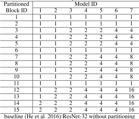
Model setting.ResNet-32 consists of 15 convolutional blocks, where each convolutional block contains two or three convolutional layers. Considering the number of possible compression configurations on different convolutional lay-ers is very large, we choose to make the laylay-ers in the same block have the same compression ratio. In other words, a
block-wisecompression strategy is adopted. Notice that be-cause the first few convolutional layers of ResNet are very sensitive for compression (He et al. 2016), in this experiment we do not impose circulant structure to the convolutional layers in the 1st and 2nd blocks of ResNet-32. Besides, the 6th and 11th blocks are not compressed due to their small weight tensor.
Table 2 shows the detailed compression configurations for different convolutional blocks of ResNet-32. Here we ex-plore 7 different compression configurations and then ob-tain 7 compressed models. For each compressed model, the compression ratios for its component convolutional blocks are listed in the row direction. Here each numberiin a spe-cific compression configuration scheme indicates the com-pression ratio asifor the convolutional layers in the corre-sponding convolutional block. When the block is associated with 1, that means the corresponding convolutional block is not compressed. Notice that due to the sensitivity of front blocks, for all the 7 models in Table 2 the compression ra-tios of the front blocks are typically less than those of the later blocks.
Trade-off between accuracy and model size.Figure 2 shows the test error for 7 compressed models. It can be seen that model 1 even achieves slightly better performance with a smaller model size than the baseline. Moreover, model 2, 3 and 4 achieve around 50% reduction in model size with negligible accuracy drop. With more aggressive compres-sion configurations are selected (such as model 5, 6 and 7), more reduction in model size can be further achieved with slight increase of test error.
Trade-off between accuracy and FLOPs. Our experi-ment also shows that the use of circulant convolutional layer helps reduce computational cost significantly. As shown in Figure 3, compressed model 1 and 2 achieve fewer FLOPs than baseline with the same or even less test error. For model 3, it can achieve 50% reduction in FLOPs with negligible
Table 2: Compression Configurations. For the convolutional block with compression ratioi, all the convolutional layers in that block has the same compression ratioi.
Partitioned Model ID
Block ID 1 2 3 4 5 6 7
1 1 1 1 1 1 1 1
2 1 1 1 1 1 1 1
3 1 1 2 2 2 4 4
4 1 1 2 2 2 4 4
5 1 1 2 2 2 4 4
6 1 1 1 1 1 1 1
7 1 1 2 2 4 4 8
8 1 1 2 2 4 4 8
9 1 1 2 2 4 4 8
10 1 1 2 2 4 4 8
11 1 1 1 1 1 1 1
12 1 2 2 4 4 4 16
13 1 2 2 4 4 4 16
14 2 2 2 4 4 4 16
15 2 2 2 4 4 4 16
baseline (He et al. 2016):ResNet-32 without partitioning
test error increase. An interesting discovery is that though model 4, 5 and 6 have more aggressive compression con-figurations than model 3, their corresponding reduction in FLOPs are less than what model 3 achieves. This is because the convolutional layers in the model 3 are mainly com-pressed with the factor of 2, which corresponds to 2-point FFT computation that only needs real number operations.
1 2
3 4
5 6 7
Baseline 7.0
7.5 8.0 8.5 9.0 9.5
80 180 280 380 480
)
%(
ror
rE
tse
T
Parameters (K) CircConv Baseline
Figure 2: ResNet-32 Test Error and Model Size. Use of cir-culant convolutional layer can bring half of parameters re-duction with negligible test error increase.
Wide ResNet on CIFAR-10
We also conduct the experiment on CIFAR-10 dataset using Wide ResNet (Zagoruyko and Komodakis 2016), which has better performance than conventional ResNet in term of test accuracy. In this experiment, the compressed Wide ResNet models are trained using SGD with learning rate 0.01, mo-mentum 0.9, batch size 64 and weight decay 0.0005.
1 2
3 4
5 6 7
Baseline
6.0 6.5 7.0 7.5 8.0 8.5 9.0 9.5 10.0
40% 50% 60% 70% 80% 90% 100%
)
%(
ror
rE
tse
T
FLOPs percentage (%) CircConv Baseline
Figure 3: ResNet-32 Test Error and Model Size. Use of cir-culant convolutional layer can bring half of FLOPs reduction with negligible test error increase.
r
Figure 4: Wide ResNet Model Size Reduction. Compared with baseline models, compressed models achieve similar model size as ResNet-110. Compressed model named like ”48-4” has 48 convolutional layers and widening parameter as 4.
(Zagoruyko and Komodakis 2016) and set different num-bers of convolutional blocks and widening parameters for different models. To achieve better performance, we add two more blocks to the convolutional blocks that are wider than
16×k, wherekis the inherent widening parameter of each block. Different from the experiment in ResNet experiment section, this experiment on Wide ResNet adopts very ag-gressive compression strategy: For one convolutional layer, if the numbers of input channels (C0) and output channels
(C2) are the same, then the compression ratio for that layer
isi = C0 = C2; otherwise the convolutional layer is not
compressed. We apply this compression strategy to five dif-ferent Wide ResNet baselines and obtain five compressed Wide ResNet models. For each compressed model, it is la-beled with two numbers (”d-k”), wheredandkdenote the number of convolutional layers (”depth”) and widening pa-rameter (”width”), respectively. These compressed models are compared with their corresponding baseline models as well as ResNet-110, which achieves the best performance on CIFAR-10 in (He et al. 2016).
Model size reduction.Figure 4 shows the number of pa-rameters of Wide ResNet baselines and the corresponding compressed models after imposing circulant structure. It can
be seen that the compressed models greatly reduce the model size. In particular, model ”60-4” can achieve 8.35 times re-duction in the model size. Also, it can be seen that the num-bers of parameters of Wide ResNet models are similar to the size of ResNet-110 after applying circulant convolutional layer. For instance, Model ”48-4” has around 1.6M parame-ters which is less than 1.7M for ResNet-110.
Test error analysis. Figure 5 shows test errors of base-line Wide ResNet models and the corresponding compressed models using circulant convolutional layer. It can be seen that all compressed models have slightly test error increase less than 1%. In addition, compared with the state-of-the-art ResNet-110, all of the compressed models have around 1% test error decrease.
Figure 5: Wide ResNet Test Error. Baseline models are dif-ferent original Wide ResNets and they are compared with the corresponding compressed models and ResNet-110.
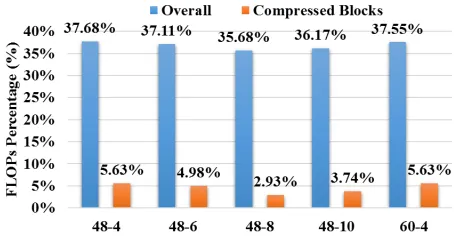
Figure 6: Wide ResNet FLOPs. The overall FLOPs measure the FLOPs percentage of compressed models over corre-sponding baselines. We also list FLOPs percentage of com-pressed convolutional blocks over original blocks.
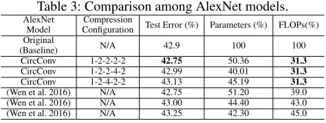
Table 3: Comparison among AlexNet models. AlexNet
Model
Compression
Configuration Test Error (%) Parameters (%) FLOPs(%) Original
(Baseline) N/A 42.9 100 100 CircConv 1-2-2-2-2 42.75 50.36 31.3
CircConv 1-2-2-4-2 42.99 40.01 31.3
CircConv 1-2-4-2-2 43.13 45.19 31.3
(Wen et al. 2016) N/A 42.75 51.20 39.0 (Wen et al. 2016) N/A 43.00 44.40 43.0 (Wen et al. 2016) N/A 43.25 42.30 45.0
FLOPs reduction.As shown in Figure 6, we measure the overall FLOPs reduction of Wide ResNet. It is found that the compressed Wide ResNet models can achieve significant reduction in FLOPs: all of them only require around 36% FLOPs as compared to the corresponding baseline models. In addition, the FLOPs reduction for the compressed blocks are very significant. From Figure 6 it can be seen that the FLOPs in the compressed blocks of all compressed models are only less than 6% of the corresponding uncompressed blocks in the original Wide ResNet baseline models.
AlexNet on ImageNet
To test the effectiveness of the proposed circulant-imposing approach on large-scale datasets, we evaluate the perfor-mance of circulant CNNs on ImageNet (ILSVRC2012). Here the baseline model is AlexNet (Krizhevsky, Sutskever, and Hinton 2012). All training images are randomly dis-torted as suggested in (Szegedy et al. 2016). We train our AlexNet models using RMSprop (Tieleman and Hinton 2012) with learning rate 0.01, momentum 0.9, batch size 32 and decay 0.9.
Model settings. We explore three different compres-sion configurations for the five convolutional layers in AlexNet. Table 3 listed the detailed compression configu-ration schemes by using notation ”a-b-c-d-e”. For instance, ”1-2-2-2-2” means the first convolutional layer is not com-pressed, and the rest four layers are compressed with the factor of 2. By using these configurations, three compressed AlexNet models are generated and compared with origi-nal AlexNet baseline model. Also, since SSL in (Wen et al. 2016) is the state-of-the-art work that explores the re-lationship between accuracy and compressed model size for AlexNet, we also compare our circulant convolutional layer-based compressed AlexNet models with three SSL regularization-based compressed AlexNet models in (Wen et al. 2016).
Test error analysis. Table 3 shows the test errors of compressed AlexNet models by using circulant structure-imposing and SSL approaches. It can be seen that both these two approaches can render the compressed models with the similar test errors to the original AlexNet model. Among them, the circulant model with ”1-2-2-2-2” compression configuration achieves the least test error.
Model size reduction.Table 3 shows the percentage of number of parameters of each model over original AlexNet model. It can be seen that circulant convolution-based els have similar numbers of parameters to SSL-based mod-els. Among them the circulant convolution-based model
with ”1-2-2-4-2” compression configuration has the least number of parameters.
FLOPs reduction. Table 3 shows the percentage of FLOPs of each model over the original AlexNet model. It can be found that all circulant convolution-based models require fewer FLOPs than the SSL regulation-based mod-els. All the circulant convolution-based models have around 31% FLOPs of original uncompressed AlexNet baseline.
Overall comparison. As shown in Table 3 , circulant convolution-based models have similar accuracy to the state-of-the-art SSL models while maintaining similar number of parameters. Meanwhile, Table 3 shows that circulant convolution-based models requires less FLOPs than the SSL models when targeting to the similar accuracy. Therefore, imposing circulant structure to convolutional layer is a very promising accuracy-retained approach to reduce both the space and computational costs.
Acknowledgement
This paper is the collaborative work with Zhe Li, Liang Zhao, Qinru Qiu and Yanzhi Wang. Their names do not ap-pear in the author list due to the mistake during submission. The authors would like to appreciate anonymous reviewers’ valuable comments and suggestions. This work is supported by the National Science Foundation Awards CCF-1854742.
Conclusion
In this paper, we propose to impose the circulant structure to convolutional neural network. This structure-imposing ap-proach leads to significant reduction in model size, FLOPs with negligible accuracy drop. Complexity analysis and ex-periments on different datasets and different network models demonstrate the effectiveness of the proposed approach.
References
Chen, W.; Wilson, J.; Tyree, S.; Weinberger, K. Q.; and Chen, Y. 2016. Compressing convolutional neural networks in the frequency domain. InProceedings of the 22nd ACM SIGKDD International Conference on Knowledge Discov-ery and Data Mining, 1475–1484. ACM.
Cheng, Y.; Yu, F. X.; Feris, R. S.; Kumar, S.; Choudhary, A.; and Chang, S.-F. 2015. An exploration of parameter redundancy in deep networks with circulant projections. In
Proceedings of the IEEE International Conference on Com-puter Vision, 2857–2865.
Chu, M. T., and Plemmons, R. J. 2003. Real-valued low rank circulant approximation. SIAM Journal on Matrix Analysis and Applications24(3):645–659.
Deng, J.; Dong, W.; Socher, R.; Li, L.-J.; Li, K.; and Fei-Fei, L. 2009. Imagenet: A large-scale hierarchical im-age database. InComputer Vision and Pattern Recognition, 2009. CVPR 2009. IEEE Conference on, 248–255. IEEE.
IEEE/ACM International Symposium on Microarchitecture, 395–408. ACM.
Feng, J., and Darrell, T. 2015. Learning the structure of deep convolutional networks. InProceedings of the IEEE International Conference on Computer Vision, 2749–2757.
Girosi, F.; Jones, M.; and Poggio, T. 1995. Regularization theory and neural networks architectures. Neural computa-tion7(2):219–269.
Gong, Y.; Liu, L.; Yang, M.; and Bourdev, L. 2014. Com-pressing deep convolutional networks using vector quantiza-tion.arXiv preprint arXiv:1412.6115.
Han, S.; Mao, H.; and Dally, W. J. 2015. Deep com-pression: Compressing deep neural networks with pruning, trained quantization and huffman coding. arXiv preprint arXiv:1510.00149.
He, K.; Zhang, X.; Ren, S.; and Sun, J. 2016. Deep residual learning for image recognition. InProceedings of the IEEE Conference on Computer Vision and Pattern Recognition, 770–778.
Jaderberg, M.; Vedaldi, A.; and Zisserman, A. 2014. Speed-ing up convolutional neural networks with low rank expan-sions. arXiv preprint arXiv:1405.3866.
Karpathy, A.; Toderici, G.; Shetty, S.; Leung, T.; Suk-thankar, R.; and Fei-Fei, L. 2014. Large-scale video clas-sification with convolutional neural networks. In Proceed-ings of the IEEE conference on Computer Vision and Pattern Recognition, 1725–1732.
Krizhevsky, A., and Hinton, G. 2009. Learning multiple layers of features from tiny images.
Krizhevsky, A.; Sutskever, I.; and Hinton, G. E. 2012. Imagenet classification with deep convolutional neural net-works. InAdvances in neural information processing sys-tems, 1097–1105.
LeCun, Y.; Bottou, L.; Bengio, Y.; and Haffner, P. 1998. Gradient-based learning applied to document recognition.
Proceedings of the IEEE86(11):2278–2324.
Mathieu, M.; Henaff, M.; and LeCun, Y. 2013. Fast train-ing of convolutional networks through ffts. arXiv preprint arXiv:1312.5851.
Moczulski, M.; Denil, M.; Appleyard, J.; and de Freitas, N. 2015. Acdc: A structured efficient linear layer. arXiv preprint arXiv:1511.05946.
Pan, V. 2012.Structured matrices and polynomials: unified superfast algorithms. Springer Science & Business Media. Rezghi, M., and Eld´en, L. 2011. Diagonalization of tensors with circulant structure.Linear Algebra and its Applications
435(3):422–447.
Sainath, T. N.; Kingsbury, B.; Sindhwani, V.; Arisoy, E.; and Ramabhadran, B. 2013. Low-rank matrix factoriza-tion for deep neural network training with high-dimensional output targets. InAcoustics, Speech and Signal Processing (ICASSP), 2013 IEEE International Conference on, 6655– 6659. IEEE.
Simonyan, K., and Zisserman, A. 2014. Very deep
convo-lutional networks for large-scale image recognition. arXiv preprint arXiv:1409.1556.
Sindhwani, V.; Sainath, T.; and Kumar, S. 2015. Structured transforms for small-footprint deep learning. InAdvances in Neural Information Processing Systems, 3088–3096. Szegedy, C.; Liu, W.; Jia, Y.; Sermanet, P.; Reed, S.; Anguelov, D.; Erhan, D.; Vanhoucke, V.; and Rabinovich, A. 2015. Going deeper with convolutions. In Proceed-ings of the IEEE Conference on Computer Vision and Pat-tern Recognition, 1–9.
Szegedy, C.; Vanhoucke, V.; Ioffe, S.; Shlens, J.; and Wojna, Z. 2016. Rethinking the inception architecture for computer vision. InProceedings of the IEEE Conference on Computer Vision and Pattern Recognition, 2818–2826.
Tieleman, T., and Hinton, G. 2012. Lecture 6.5-rmsprop: Divide the gradient by a running average of its recent mag-nitude.COURSERA: Neural networks for machine learning
4(2):26–31.
Wang, Y.; Xu, C.; You, S.; Tao, D.; and Xu, C. 2016. Cn-npack: packing convolutional neural networks in the fre-quency domain. InAdvances in neural information process-ing systems, 253–261.
Wang, Y.; Ding, C.; Li, Z.; Yuan, G.; Liao, S.; Ma, X.; Yuan, B.; Qian, X.; Tang, J.; Qiu, Q.; et al. 2018. Towards ultra-high performance and energy efficiency of deep learn-ing systems: an algorithm-hardware co-optimization frame-work. InAssociation for the Advancement of Artificial Intel-ligence.
Wen, W.; Wu, C.; Wang, Y.; Chen, Y.; and Li, H. 2016. Learning structured sparsity in deep neural networks. In
Advances in Neural Information Processing Systems, 2074– 2082.
Zagoruyko, S., and Komodakis, N. 2016. Wide residual networks. arXiv preprint arXiv:1605.07146.
Zhao, L.; Liao, S.; Wang, Y.; Tang, J.; and Yuan, B. 2017. Theoretical properties for neural networks with weight matrices of low displacement rank. arXiv preprint arXiv:1703.00144.