The Thirty-Third AAAI Conference on Artificial Intelligence (AAAI-19)
Collaborative, Dynamic and Diversified User Profiling
Shangsong Liang
1,21School of Data and Computer Science, Sun Yat-sen University, China
2Guangdong Key Laboratory of Big Data Analysis and Processing, Guangzhou 51006, China
Abstract
In this paper, we study the problem of dynamic user profiling in the context of streams of short texts. Previous work on user profiling works with long documents, do not consider collab-orative information, and do not diversify the keywords for profiling users’ interests. In contrast, we address the problem by proposing a user profiling algorithm (UPA), which con-sists of two models: the proposed collaborative interest track-ing topic model (CITM) and the proposed streamtrack-ing keyword diversification model (SKDM). UPA first utilizes CITM to collaboratively track each user’s and his followees’ dynamic interest distributions in the context of streams of short texts, and then utilizes SKDM to obtain top-krelevant and diversi-fied keywords to profile users’ interests at a specific point in time. Experiments were conducted on a Twitter dataset and we found that UPA outperforms state-of-the-art non-dynamic and dynamic user profiling algorithms.
Introduction
To capture users’ dynamic interests underlying their posts in microblogging platforms such as Twitter is of impor-tance to the success of further design of applications that cater for users of such platforms, such as dynamic user clustering (Liang et al. 2017a; 2017b). In this paper, we study the problem of user profiling for streaming short documents (Balog et al. 2012; Liang 2018; Liang et al. 2018): collaboratively identifying users’ dynamic interests and tracking how they evolve over time in the context of streaming short texts. Our goal is to infer users’ and their collaborative topic distributions over time and dynamically profile their interests with a set of diversified keywords in the context of streaming short texts.
The first user profiling model was proposed in (Balog et al. 2007), where a set of relevant keywords were identified for each user in a static collection of long documents and the dynamics of users’ interests were ignored. Recent work re-alize the importance of capturing users’ dynamic interests over time and a number of temporal profiling algorithms have been proposed for streams of long documents. How-ever, previous work on user profiling suffer from the fol-lowing problems: (1) They work with streams of long doc-uments rather than short docdoc-uments and made the
assump-Copyright c2019, Association for the Advancement of Artificial Intelligence (www.aaai.org). All rights reserved.
tion that the content of documents is rich enough to infer users’ dynamic interests. (2) They ignore any collaborative information, such as friends’ messages when inferring users’ interests at a specific point in time. (3) They just simply re-trieve a list of top-kkeywords as a user’s profile that may be semantically similar to each other and thus redundant.
Accordingly, in this paper, to address the aforementioned drawbacks in the previous work, we propose a User Profil-ing Algorithm in the context of streams of short documents, abbreviated asUPA, which iscollaborative, dynamic and di-versified. UPA consists of two proposed models– a Collabo-rative Interest Tracking topic Model, abbreviated asCITM, and a Streaming Keyword Diversification Model, abbrevi-ated as SKDM. UPA algorithm first utilizes our proposed CITM to track the changes of users’ dynamic interests in the context of streams of short documents. It then utilizes our proposed SKDM to produce top-kdiversified keywords for profiling users’ interests at a specific point in time.
Our CITM topic model works with streaming short texts and is a dynamic multinomial Dirichlet mixture topic model that is able to infer and track each user’s dynamicinterest distributions based not only on the user’s posts but also the
collaborativeinformation, i.e., his followees’ posts. Our hy-pothesis in CITM is that accounting for collaborative infor-mation is critical, especially for those users with limited ac-tivities, infrequent short posts, and thus sparse information. To perform the inference of users’ interest distributions in streams of short documents, we propose a collapsed Gibbs sampling algorithm. Then, our SKDM model works with users’ dynamic interest distributions produced by CITM and aims at retrieving a set of relevant and alsodiversified key-words for profiling users’ interests at timetsuch that redun-dancy of the retrieved keywords can be avoided while still keeping relevant keywords to profile the users.
Related Work
User Profiling.User profiling has been gaining attention af-ter the launch of user finding task at TREC 2005 enaf-terprise track (Craswell, de Vries, and Soboroff 2005). Balog and de Rijke (2007) worked with a static long document corpus and modeled the profile of a user as a set of relevant key-words. Recent work were aware of the importance of tem-poral user profiling. Temtem-poral profiling for long documents was first introduced in (Rybak, Balog, and Nørv˚ag 2014), where topical areas were organized in a predefined taxon-omy and interests were represented as a weighted unchanged tree built by the ACM classification system. A probabilistic model was proposed in (Fang and Godavarthy 2014), where experts’ academic publications were used to investigate how personal interests evolve over time. We follow most previous work, and retrieve top-kwords as profile of a user’s interests. Topic Modeling.Topic models provide a suite of algorithms to discover hidden thematic structure in a collection of docu-ments. A topic model takes a set of documents as input, and discovers a set of “latent topics”—recurring themes that are discussed in the collection—and the degree to which each document exhibits those topics (Blei, Ng, and Jordan 2003). Since the well-known topic models, PLSI (Probabilistic La-tent Semantic Indexing) (Hofmann 1999) and LDA (LaLa-tent Dirichlet Allocation) (Blei, Ng, and Jordan 2003), were pro-posed, topic models with dynamics have been widely stud-ied. These include Dynamic Topic Model (Blei and Laf-ferty 2006), Dynamic Mixture Model (Wei, Sun, and Wang 2007), Topic over Time (Wang and McCallum 2006), Topic Tracking Model (Iwata et al. 2009), and more recently, dy-namic Dirichlet multinomial mixture topic model (Liang et al. 2017c), user expertise tracking topic model (Liang 2018) and user collaborative interest tracking topic model (Liang, Yilmaz, and Kanoulas 2018). To our knowledge, none of ex-isting dynamic topic models has considered the problem of user profiling for short texts that utilizes collaborative infor-mation to infer topic distributions.
Problem Formulation
We follow most of the previous work (Balog and de Rijke 2007; Berendsen et al. 2013; Liang et al. 2018), and retrieve top-kwords as profile of a user. Then, the problem we ad-dress in this paper is: given a set of users and streams of short documents generated by them, track their interests over time and dynamically identify a set of top-krelevant and di-versified keywords to each of the users. The dynamic user profiling algorithm is essentially a functionhthat satisfies:
Dt,ut h −→Wt,
where Dt = {. . . ,dt−2,dt−1,dt} represents the stream
of short documents generated by the usersutup to timet with dt being the most recent set of short documents ar-riving at t, ut = {u1, u2, . . . , u|ut|} represents a set of
users appearing in the stream up to time t, with ui be-ing thei-th user inut and|ut|being the total number of users in the user set, andWt={wt,u1,wt,u2, . . . ,wut,|ut|}
represents all users’ profiling results at t with wt,ui =
{wt,ui,1, wt,ui,2, . . . , wt,ui,k}being the profiling result, i.e.,
the top-kdiversified keywords, for useruiatt. We assume that the length of a documentdinDtis no more than a pre-defined small length (e.g., 140 characters in Twitter).
User Profiling Algorithm
In this section, we detail our proposed User Profiling Al-gorithm (UPA) that consists of the proposed Collaborative Interest Tracking topic Model (CITM) and the proposed Streaming Keyword Diversification Model (SKDM).
Overview
We model users’ interests in streams by latent topics. There-fore, the dynamic interests of each useru∈utat time pe-riodtcan be represented as a multinomial distributionθt,u over topics, whereθt,u ={θt,u,z}Zz=1withθt,u,zbeing the interest score on topiczfor useruat time periodtandZ be-ing the total number of latent topics. Similarly, the dynamic interests of each user’s followees attcan be represented as a multinomial distributionψt,u = {ψt,u,z}Zz=1withψt,u,z being the interest score of useru’s followeesft,uas a whole on topiczatt. Here,ft,udenotes useru’s all followees att. Our UPA algorithm consists of two main steps: (1) UPA first utilizes the proposed CITM to capture each user’s dy-namic interestsθt,uand his collaborative interestsψt,u. (2) Givenθt,uandψt,uhaving been inferred, UPA then utilizes SKDM to identify top-krelevant and diversified keywords for profiling the useru’s dynamic interests at time periodt.
Collaborative Interest Tracking Model
Modeling Interests over Time. We close follow the pre-vious work in (Liang, Yilmaz, and Kanoulas 2018; Liang et al. 2017a), and aim at inferring each user’s dynamic in-terest distributionθt,u ={θt,u,z}Z
z=1and his collaborative interest distributionψt,u = {ψt,u,z}Z
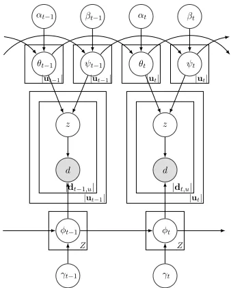
z=1 attin the context of streams of short documents in our CITM. We provide CITM’s graphical representation in Fig. 1.
To track the dynamics of a useru’s interests, we assume that the mean of his current interests θt,u at time period t is the same as that att−1, unless otherwise newly arrived documents associated with the useruin the streams can be observed. With this assumption and following the previous work on dynamic topic models (Iwata et al. 2010; 2009; Wei, Sun, and Wang 2007), we use the following Dirichlet prior with a set of precision valuesαt={αt,z}Zz=1, where we let the mean of the current distributionθt,udepend on the mean of the previous distributionθt−1,uas:
P(θt,u|θt−1,u,αt)∝ Z
Y
z=1
θαt,u,zθt−1,u,z−1
t,u,z , (1)
θt−1 αt−1
ψt−1 βt−1
θt αt
ψt βt
z z
d d
φt−1 φt
γt−1 γt
Z Z
|ut−1| |ut−1| |ut| |ut|
|dt−1,u| |dt,u|
|ut−1| |ut|
Figure 1: Graphical representation of our proposed CITM model. Shaded nodes represent observed variables.
the following Dirichlet prior with a set of precision values βt={βt,z}Z
z=1, where the mean of the current distribution ψt,uevolves from that of the previous distributionβt−1,u:
P(ψt,u|ψt−1,u,βt)∝
Z
Y
z=1
ψβt,u,zψt−1,u,z−1
t,u,z , (2)
where the precision value βt,z = {βt,u,z}|uu=1t| represents the persistency of users’ collaborative interest, which is how saliency topiczis at time periodtin contrast to that att−1
for the users. In a similar way, to model the dynamic changes of the multinomial distribution of words specific to topicz, we assume a Dirichlet prior, in which the mean of the cur-rent distributionφt,z={φt,z,v}V
v=1evolves from the mean of the previous distributionφt−1,z:
P(φt,z|φt−1,z,γt)∝ V
Y
v=1
φγt,z,vφt−1,z,v−1
t,z,v , (3)
whereV is the total number of words in a vocabularyv =
{vi}V
i=1 andγt= {γt,v} V
v=1, withγt,v = {γt,z,v} Z z=1 rep-resenting the persistency of the wordvin all topics at timet, a measure of how consistently the word belongs to the top-ics attcompared to that att−1. Later in this subsection, we propose a collapsed Gibbs sampling algorithm to infer all users’ dynamic interest distributionsΘt = {θt,u}|uu=1t|, their corresponding dynamic collaborative interest distribu-tionsΨt = {ψt,u}
|ut|
u=1, and the words’ dynamic topic dis-tributionsΦt={φt,z}Zz=1, and describe our update rules to obtain the optimal persistency valuesαt,βtandγt.
Assume that we know all users’ interest distribution at timet−1,Θt−1, their collaborative interest distribution at
timet−1,Ψt−1, and the words’ topic distribution,Φt−1.
Then the proposed collaborative interest tracking model is essentially a generative topic model that depends onΘt−1,
Algorithm 1:Inference for our CITM model at timet. Input :DistributionsΘt−1,Ψt−1andΦt−1att−1;
Initializedαt,βtandγt; Number of iterations Niter.
Output:Current distributionsΘt,ΨtandΦt.
1 Initialize topic assignments randomly for all documents
indt
2 foriteration= 1 toNiterdo 3 foruser= 1 to|ut|do
4 ford= 1 todt,udo
5 Drawzt,u,dfrom (5)
6 Updatemt,u,zt,u,d,ot,u,zt,u,dandnt,zt,u,d,v
7 Updateαt,βtandγt
8 Compute the posterior estimatesΘt,ΨtandΦt.
Ψt−1 andΦt−1. For initialization and without loss of gen-eralization, we letθ0,u,z= 1/Z,ψ0,u,z= 1/Zandφ0,z,v= 1/V att = 0. Let all the short documents posted by user uat time periodtdenote asdt,u. The generative process of our model for documents in stream at timet, is as follows,
i. DrawZ multinomialsφt,z, one for each topicz, from a Dirichlet prior distributionγt,zφt−1,z;
ii. For each useru∈ut, draw multinomialsθt,uandψt,u from Dirichlet distributions with priorsαt,uθt−1,uand βt,uψt−1,u, respectively;
iii. For each documentd∈dt,u, draw a topiczdbased on the mixture ofθt,uandψt,u, and then for each wordvd in the documentd:
(a) Draw a wordvdfrom multinomialφt,zd.
In the above generative process, given the documents in streams are short, and because most of the short documents are likely to talk about one single topic only (Yin and Wang 2014),we let all the words in the same documentdbe drawn from the multinomial distribution associated with the same topiczd. See the graphical representation of CITM in Fig. 1.
Interest Distribution Inference. We propose a collapsed Gibbs sampling algorithm that is based on the basic col-lapsed Gibbs sampler (Griffiths and Steyvers 2004; Wallach 2006) to approximately infer the distributions in our CITM topic model. As shown in Fig. 1 and the generative process, we adopt a conjugate prior (Dirichlet) for the multinomial distributions, and thus we can easily integrate out the uncer-tainty associated with multinomialsθt,u,ψt,uandφt,z.
We provide an overview of our proposed collapsed Gibbs sampling algorithm in Algorithm 1, where we de-note mt,u,z, ot,u,z and nt,z,v to be the number of doc-uments assigned to topic z for user u, the number of documents assigned to topic z for user u’s followees and the number of times word v assigned to topic z for user u at t, respectively. In the Gibbs sampling pro-cedure, we need to calculate the conditional distribution P(zt,u,d|zt,−(u,d),dt,Θt−1,Ψt−1,Φt−1,ut,αt,βt,γt)at time t, where zt,−(u,d) represents the topic assignments for all the documents in dt except the document d ∈
assigned to the document d ∈ dt,u. For obtaining this conditional distribution used during sampling, we begin with the joint probability of the current document set, P(zt,dt|Θt−1,Ψt−1,Φt−1,ut,αt,βt,γt)at timet:
P(zt,dt|Θt−1,Ψt−1,Φt−1,ut,αt,βt,γt) (4) = (1−λ)P(zt,dt|Θt−1,Φt−1,ut,αt,γt)
=+λP(zt,dt|Ψt−1,Φt−1,ut,βt,γt)
= (1−λ)Y
z
Γ(P v(κb)) Q
vΓ(κb) Q
vΓ(κa)
Γ(P vκa)
! ·Y
u
Γ(P z(κ2))
Q zΓ(κ2)
Q zΓ(κ1)
Γ(P zκ1)
=+λY
z
Γ(P v(κb)) Q
vΓ(κb) Q
vΓ(κa)
Γ(P vκa)
! ·Y
u
Γ(P z(κ4))
Q zΓ(κ4)
Q zΓ(κ3)
Γ(P zκ3)
,
whereΓ(·)is a gamma function,λis a free parameter that governs the linear mixture of a user’s interests and his fol-lowees’ interests, and the set of parametersκare defined as:
κ1 = mt,u,z+αt,zθ,κ2 = αt,u,zθ,κ3 =ot,u,z +βt,zψ,
κ4 = βt,u,zψ, κa = nt,z,v +γt,vφ, and κb = γt,z,vφ. Here, we let θ, ψ and φabbreviate for θt−1,u,z, ψt−1,u,z andφt−1,z,v, respectively. Based on the above joint
distribu-tion (4) and using the chain rule, we can obtain the following conditional distribution conveniently for the proposed Gibbs sampling (step 5 of Algorithm 1) as the following:
P(zt,u,d=z|zt,−(u,d),dt,Θt−1,Ψt−1,Φt−1,ut,αt,βt,γt) =
(1−λ) mt,u,z+αt,u,zθ−1
PZ
z=1(mt,u,z+αt,u,zθ)−1 +
λ ot,u,z+βt,u,zψ−1
PZ
z=1(ot,u,z+βt,u,zψ)−1
× Q
v∈d
QNd,v
j=1(nt,z,v,−(u,d)+γt,z,vφ+j−1) QNd
i=1(nt,z,−(u,d)+i−1 +PVv=1γt,z,vφ)
, (5)
whereNd,Nd,v,zt,−(u,d),nt,z,v,−(u,d)andnt,z,−(u,d) are the length of documentd, the number of wordv appearing ind, topic assignments for all documents except the doc-ument dfrom useruatt, the number of wordv assigned to topicz in all documents except the one from user uat t, and the number of documents assigned to zin all docu-ments except the one from useruatt, respectively. At each iteration during the sampling (steps 2 to 7 of Algorithm 1), the precision parametersαt,βtandγtcan be estimated by maximizing the joint distribution (4). We apply fixed-point iterations to obtain the optimalαt,βtandγt. By applying the two bounds in (Minka 2000), we can derive the follow-ing update rules ofαt,βtandγtfor maximizing the joint distribution in our fixed-point iterations:
αt,u,z←(1−λ)αt,u,z ∆(mt,u,z+αt,u,zθ)−∆(αt,u,zθ)
∆(PZ
z=1mt,u,z+αt,u,zθ)−∆(
PZ
z=1αt,u,zθ)
,
βt,u,z← λβt,u,z ∆(ot,u,z+βt,u,zψ)−∆(βt,u,zψ)
∆(PZ
z=1ot,u,z+βt,u,zψ)−∆(
PZ
z=1βt,u,zψ)
, (6)
γt,z,v← γt,z,v ∆(nt,z,v+γt,z,vφ)−∆(γt,z,vφ)
∆(PV
v=1nt,z,v+γt,z,vφ)−∆(
PV
v=1γt,z,vφ)
,
where ∆(x) = ∂logxΓ(x) is a Digamma function. Our derivations of the update rules forαt,βtandγtin (6) are analogous to those in (Liang, Yilmaz, and Kanoulas 2018; Liang et al. 2017c; 2017b).
After the Gibbs sampling is done, with the fact that Dirichlet distribution is conjugate to multinomial tion, we can conveniently infer each user’s interest distribu-tionθt,u, his collaborative interest distributionψt,uand the
Algorithm 2:SKDM model for generating top-k key-words for collaborative, dynamic, diversified user profil-ing.
Input :Current distributionsΘtandΦt Output:All users’ profiling results at timet,Wt
1 foru= 1, . . . ,|ut|do
2 wt,u←∅ /* wt,u∈Wt */
3 e v←v
4 forz= 1, . . . , Zdo
5 δt,u,z ←(1−λ)P(z|t, u) +λP(z|t,ft,u)
6 sz|t,u←0
7 forall positions in the ranked listwt,u do
8 forz= 1, . . . , Zdo
9 qt[z|t, u] = 2sδt,u,z z|t,u+1 10 z∗←arg maxzqt[z|t, u] 11 v∗←arg maxv∈ev η1×qt[z
∗|t, u]×
P(v|t, z∗) +η
2Pz6=z∗qt[z|t, u]×
P(v|t, z) + (1−η1−η2)×tfidf(v|t, u) 12 wt,u←wt,u∪ {v∗} /* append v∗ to
wt,u */
13 ve←ev\{v∗} /* remove v∗ from ve */
14 forz= 1, . . . , Zdo
15 sz|t,u←sz|t,u+ P(v
∗|t,u) PZ
z0=1P(v
∗|t,z0)
words’ topic distributionφt,zatt, respectively as:θt,u,z = mt,u,z+αt,u,z
PZ
z0=1mt,u,z0+αt,u,z0, ψt,u,z =
ot,u,z+βt,u,z
PZ
z0=1ot,u,z0+βt,u,z0, and
φt,z,v=
nt,z,v+γt,z,v
PV
v0=1nt,z,v0+γt,z,v0
.
Streaming Keyword Diversification Model
After we obtainθt,u,ψt,u andφt,z, inspired by PM-2 di-versification method (Dang and Croft 2012), we closely fol-low the work in (Liang et al. 2017c; 2018) and propose a streaming keyword diversification model (i.e., Algorithm 2), SKDM. To generate top-kdiversified keywords for each user uatt, SKDM starts with an empty keyword setwt,uwith k empty seats (step 2 of Algorithm 2), and a set of candi-date keywords (step 3),ve, which is the whole wordsvin the vocabulary, i.e., initially let ve = v. For each of the seats, it computes the quotient qt[z|t, u] for each topic z given a user uatt by the Sainte-Lagu¨e formula (step 9): qt[z|t, u] = δt,u,z
2sz|t,u+1, whereδt,u,z is the final probability
of the user u has interest on topic z at t and is set to be δt,u,z = (1−λ)P(z|t, u) +λP(z|t,ft,u)(step 5), andsz|t,u is the “number” of seats occupied by topicz(in initializa-tion, let sz|t,u = 0 for all topics (step 6)). HereP(z|t, u) andP(z|t,ft,u)are the probabilities of useru’s own and his collaborative interest on topiczatt, respectively. Obviously, we can obtainP(z|t, u)andP(z|t,ft,u)by our CITM algo-rithm such thatP(z|t, u) =θt,u,z andP(z|t,ft,u) =ψt,u,z, i.e., we have:
whereδt,u = {δt,u,z}Z
z=1 is useru’s final interest distri-butions inferred based on his own and his collaborative in-formation at timet. According to the Sainte-Lagu¨e method, seats should be awarded to the topic with the largest quo-tient in order to best maintain the proportionality of the re-sult list. Therefore, our SKDM assigns the current seat to the topicz∗with the largest quotient (step 10). The keyword to fill this seat is the one that is not only relevant to topicz∗ but to other topics and should be specific to the user, and thus we propose to obtain the keywordv∗ for useru’s pro-filing attas (step 11):v∗←arg maxv∈evη1×qt[z
∗|t, u]×
P(v|t, z∗) +η2× P
z6=z∗qt[z|t, u]×P(v|t, z)
+ (1− η1−η2)×tfidf(v|t, u), where0≤η1, η2≤1are two free parameters that satisfy0 ≤ η1+η2 ≤ 1,P(v|t, z)is the probability thatv is associated with topicz at time t and thus can be set to beP(v|t, z) = φt,z,v, andtfidf(v|t, u)is a time-sensitive term frequency-inverse document frequency function for useruatt, which can be defined as:
tfidf(v|t, u) = tf(v|dt,u)×idf(v|u,dt), (8)
wheretf(v|dt,u) =
|{d∈dt,u:v∈d}|
|dt,u| is a term frequency
func-tion that computes how many percents of the documents that contain the word v in the whole document set dt,u, andidf(v|u,dt) = log|{d∈dt|d:vt|∈d}|+ is an inverse docu-ment frequency function withbeing set to1to avoid the division-by-zero error. According to (8), ifvfrequently ap-pears in the document setdt,ugenerated by userubut not frequently appears in the document setdtgenerated by all the users, tfidf(v|t, u) will return a high score. After the word v∗ is selected, SKDM adds v∗ as a result keyword to wt,u, i.e., wt,u ← wt,u ∪ {v∗} (step 12), removes it from the candidate word setev, i.e.,ve←ve\{v∗}(step 13),
and increases the “number” of seats occupied by each of the topicsz by its normalized relevance tov∗ as (step 15): sz|t,u←sz|t,u+
P(v∗|t,u)
PZ z0=1P(v
∗|t,z0). The process (steps 7 to 15)
repeats until we get k diversified keywords. The order in which a keyword is appended towt,u determines its rank-ing for the profilrank-ing. After the process is done, we obtain a set of diversified keywordswt,uthat profile the useruatt.
Experimental Setup
Research Questions
The research questions guiding the remainder of the pa-per are: (RQ1)How does UPA perform for user profiling compared to state-of-the-art methods?(RQ2)How does the contribution of the proposed interest tracking topic model, CITM, to the overall performance of UPA? (RQ3) What is the contribution of the collaborative information for user profiling?(RQ4)What is the impact of the length of the time intervals,ti−ti−1, in UPA?
Dataset
We work with a dataset collected from Twitter.1It contains
1,375 active randomly selected users and their tweets posted
1
Crawled from https://dev.twitter.com/.
from the beginning of their registrations up to May 31, 2015. According to the statistics, most of the users are being fol-lowed by 2 to 50 followers. In total, we have 7.52 mil-lion tweets with timestamps including those from users’ fol-lowees’. The average length of the tweets is 12 words.
We use this dataset as our stream of short documents. We obtain two categories of GroundTruths: one for evaluat-ingRelevance-oriented (RGT) performance and another for evaluatingDiversity-oriented (DGT) performance. To create the RGT ground truth, we split the dataset into 5 different partitions of time periods, i.e., a week, a month, a quarter, half a year and a year, respectively. For each Twitter user at every specific time period, an annotator was asked to gen-erate a ranked list of top-k relevant keywords (k were de-cided by the annotators) as the user’s profile. In total, 68 annotators took part in the labelling with each of them la-belled about 5 Twitter user for these 5 different partitions. To create the ground truth for diversity evaluation, DGT, as it is expensive to manually obtain aspects of the keywords from annotators, we cluster the relevant keywords with their embeddings2 into 15 categories3 by k-means (MacQueen
1967). Relevant keywords within a cluster are regarded as being relevant to the same aspect in the DGT ground truth.
Baselines
We make comparisons between our UPA and the follow-ing state-of-the-art baseline algorithms: (1)tfidf.It simply utilizes (8), i.e., the content of users’ documents to retrieve top-kkeywords as profiles for the users. (2)Predictive Lan-guage Model (PLM). It models the dynamics of personal interests via a probabilistic language model (Fang and Go-davarthy 2014). (3) Latent Dirichlet Allocation (LDA). This model (Blei, Ng, and Jordan 2003) infers topic distri-butions specific to each document via the LDA model. (4) Author Topic model (AuthorT).This model (Rosen-Zvi et al. 2004) infers topic distributions specific to each user in a static dataset. (5) Dynamic Topic Model (DTM). This dynamic model (Blei and Lafferty 2006) utilizes a Gaus-sian distribution for inferring topic distribution of long doc-uments in streams. (6)Topic over Time model (ToT).This dynamic model (Wang and McCallum 2006) normalizes timestamps of long documents in a collection and then infers topics distribution for each document. (7)Topic Tracking Model (TTM).This dynamic model (Iwata et al. 2009) cap-tures the dynamic topic distributions of long documents ar-riving at timetin streams of long documents. (8)GSDMM. This is a Gibbs Sampling-based Dirichlet Multinomial Mix-ture model that assigns one topic for each short document in a static collection (Yin and Wang 2014).
For fair comparisons, the topic model baselines, GS-DMM, TTM, ToT, DTM and LDA, use both each user’s interestsθt,u and their collaborative interests for profiling. As these baselines can not directly infer collaborative inter-est distributions, we use the average interinter-ests of the user’s
2
Publicly available from https://nlp.stanford.edu/projects/ glove/.
3
followees as his collaborative interest distribution. Thus, unlike (7), in these baselines we use the mixture interests δt,u = (1−λ)θt,u+λ|ft,u|1 Pu0∈f
t,uθt,u
0 for
represent-ing each user’s final interest distribution with θt,u being inferred by the corresponding baseline topic models. The baselines, tfidf, PLM and AuthorT, are static profiling al-gorithms, while the others are dynamic. Again, for fair com-parisons, UPA and all the other topic models use our SKDM algorithm to obtain the top-k keywords. We set the num-ber of topics Z = 20 in all the topic models. For tun-ing parameters,λ,η1andη2, we use a 70%/20%/10% split for our training, validation and test sets, respectively. The train/validation/test splits are permuted until all users were chosen once for the test set. We repeat the experiments10
times and report the average results.
For further analysis of the contribution of collaborative interestsψt,u inferred by our CITM model to the profiling, we use another baseline denoted as UPAavg, in whichδt,uis set to be(1−λ)θt,u+λ|ft,u|1 P
u0∈ft,uθt,u0withθt,ubeing
inferred by CITM. Note that we still denote the proposed profiling algorithm using (7) as UPA.
Evaluation Metrics
We use standard relevance-oriented evaluation metrics, Pre@k(Precision atk), NDCG@k(Normalized Discounted Cumulative Gain atk), MRR@k(Mean Reciprocal Rank at k), and MAP@k(Mean Average precision atk) (Croft, Met-zler, and Strohman 2015), and diversity-oriented metrics, Pre-IA@k(Intent-Aware Pre@k) (Agrawal et al. 2009), α-NDCG@k(Clarke et al. 2008), MRR-IA@k(Agrawal et al. 2009), MAP-IA@k(Agrawal et al. 2009). We also propose semantic versions of the original metrics, denoted as Pre-S@k, NDCG-Pre-S@k, MRR-Pre-S@k, MAP-Pre-S@k, Pre-IA-Pre-S@k, α-NDCG-S@k, MRR-IA-S@k, and MAP-IA-S@k, respec-tively. Here the only difference between the original metrics and the corresponding semantic ones is the way to compute the relevance score of a retrieval keywordv∗to ground truth keywordvgt. For original metrics, we let the relevance score be1 if and only ifv∗ = vgt, otherwise be0; whereas for the semantic versions, we let the relevance score be the co-sine similarity between the word embedding vectors ofv∗ andvgt. Since we usually choose not too many keywords to describe a user’s profile, we compute the scores at depth 10, i.e., letk= 10. For all the metrics we abbreviateM@kas M, whereM is one of the metrics.
Results and Discussions
In this section, we analyse our experimental results.
Overall Performance
We start by answering research questionRQ1. The follow-ing findfollow-ings can be observed from Tables 1 and 2: (1) In terms of both relevance and diversity, all the topic model-based profiling algorithms, i.e., UPA, UPAavg, GSDMM, ToT, TTM, DTM, AuthorT and LDA, outperform traditional algorithms, i.e., PLM and tfidf, which demonstrates that topic modeling does help to profile users’ interests. (2) UPA and UPAavg outperform all the baseline models in terms of
Table 1: Relevance performance of UPA, UPAavg and the baselines using time periods of each month. Statistically sig-nificant differences between UPAavgand GSDMM, and be-tween UPA and UPAavgare marked in the upper right hand corner of UPAavg’s and UPA scores, respectively. Statistical significance is tested using a two-tailed paired t-test and is denoted usingNforα=.01, andMforα=.05.
Pre NDCG MRR MAP Pre-S NDCG-S MRR-S MAP-S
tfidf .254 .229 .375 .135 .409 .392 .853 .203
PLM .273 .239 .668 .140 .417 .398 .870 .212
LDA .281 .252 .674 .142 .424 .407 .878 .217
AuthorT .288 .260 .674 .145 .429 .408 .897 .220
DTM .295 .270 .694 .153 .436 .419 .883 .226
TTM .301 .276 .728 .156 .440 .426 .882 .228
ToT .312 .283 .744 .158 .445 .428 .884 .230
GSDMM .321 .301 .746 .163 .452 .437 .891 .236
UPAavg .367N .361N .840N .195N .483N .468N .939N .262N
UPA .399N .398N .860N .211N .501N .490N .946M .274N
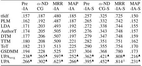
Table 2:Diversificationperformance of UPA, UPAavgand the baselines using time periods of every month. Notational conventions for the statistical significances are as in Table 1.
Pre α-ND MRR MAP Pre α-ND MRR MAP
-IA CG -IA -IA -IA-S CG-S -IA-S -IA-S
tfidf .157 .187 .480 .185 .257 .325 .725 .150
PLM .162 .192 .487 .187 .265 .332 .742 .152
LDA .171 .203 .493 .192 .272 .338 .744 .155
AuthorT .174 .205 .505 .195 .276 .343 .748 .157
DTM .177 .206 .507 .197 .279 .347 .748 .159
TTM .180 .208 .509 .221 .282 .351 .751 .162
ToT .182 .213 .513 .225 .290 .355 .754 .170
GSDMM .194 .228 .525 .237 .304 .368 .780 .173
UPAavg .238N .265N .597N .252N .362N .421N .808N .216N
UPA .266N .302N .623N .266N .395N .452N .814M .231N
relevance and diversity on all the metrics, which confirms the effectiveness of the proposed user profiling algorithm for the task. (3) The ordering of the methods, UPA>UPAavg> GSDMM >ToT∼ TTM∼DTM∼ AuthorT ∼LDA> PLM > tifdf, is mostly consistent across the two ground truths and on the relevance and diversity evaluation metrics. Here A>B denotes that methodAstatistically significantly performs better than method B and A ∼ B denotes that we did not observe a significant difference betweenAand B. This, once again, confirms that UPA and its averaged version, UPAavg, outperform all the baselines. (4) In most cases, UPA > UPAavg holds, which confirms that the col-laborative information inferred by the proposed topic model, CITM, does help to improve the profiling performance.
Additionally, Table 3 shows the top six keywords of an example user’s dynamic profile with time being five quar-ters from April 2014 to May 2015. As shown in the table, the diversified keywords generated by UPA are semantically closer to those from the ground truth compared to those gen-erated by the baseline, GSDMM, which again demonstrates the effectiveness of the proposed UPA algorithm.
Contribution of CITM
Table 3: Top six keywords of an example user’s dynamic profile with the time being five quarters from April 2014 to May 2015. The keywords from the DGT ground truth, generated from GSDMM and UPA are presented for the user, respectively.
Apr. 2014 to
Jun. 2014
Jul. 2014 to Sep. 2014 Oct. 2014 to Dec. 2014
Jan. 2015 to
Mar. 2015
Apr. 2015 to May 2015
Ground Truth
Apple Java iPhone
Python ApplePay
OjectiveC
Apple Git iPad Ojec-tiveC AppleEvent Python
AppleEvent Linin-Profile openEduca-tion iOS NatsTwitter Education
Microblog Students LinkedInProfile ArtsEducation FB AfterSchool
SocialMedia Edu-cation NatsTwitter ConnectedLearning FB Courses
GSDMM Apple Computer
iPhone Science Java Technology
Apple Company Uni-versity Technology iPad Language
Apple Christmas
LinkedIn Education iOS Friends
Online Education Students Website Degree Presentation
Courses Online Pre-sentation Digital Learning Education
UPA Apple Java iPhone
Programming CPlus-Plus Computer
Apple Programming iPad Git Event Python
Apple LinkedIn Ed-ucation iOS Twitter Education
LinkedIn Students Microblog Education FB Art
Education Media
Learning FB Courses Twitter
interests and then our SKDM to diversify the keywords, whereas other topic models utilize different topic models to obtain users’ interests and then the SKDM for keyword diversification. As in Tables 1 and 2, UPA/UPAavg outper-forms all the topic models, i.e., GSDMM, ToT, TTM, DTM AuthorT and LDA, which illustrates that the proposed topic model, CITM, does be effective and has significant contri-bution to the performance of our user profiling algorithm.
Contribution of Collaborative Interests
Here we turn to answer research questionRQ3. We vary the parameterλthat governs how much the collaborative infor-mation,ψt,u, are utilized for profiling. A largerλindicates more collaborative information is utilized for the profiling.
Fig. 2 shows the performance on the relevance and di-versity evaluation metrics (use Precision and Pre-IA as rep-resentative metrics only), where we use the best baseline, GSDMM, as a representative. When we increaseλfrom0
to0.6, i.e., giving more weight to the collaborative informa-tion, the performance of all the models gradually improves, with UPA still outperforming UPAavg and GSDMM. This, again, illustrates that integrating collaborative information into the models helps to improve the performance. More-over, as shown in Fig. 2, UPA that utilizes collaborative interests outperforms UPAavgthat simply utilizes the aver-age of the followees’ interests as its collaborative interests, which once again demonstrates that the inferred collabora-tive interests in UPA is effeccollabora-tive.
Impact of Time Period Length
Finally, we answer research questionRQ4. We compare the performance for different time periods, a week, a month, a quarter, half a year and a year, respectively, using the two ground truths, RGT and DGT, on the representative rele-vance and diversity metrics, Precision and Pre-IA, in Fig. 3. As is shown in Fig. 3, UPA and UPAavg beat the base-lines for time periods of all lengths, which illustrates that our proposed user profiling algorithm works better than the state-of-the-art ones for dynamic user profiling regardless of period length. The performance of UPA, UPAavg and the best baseline, GSDMM, improves significantly on all the metrics when the period length increases from a week to a
λ
Precision
UPA UPAavg GSDMM
0.0 0.2 0.4 0.6 0.8 1.0
0.25
0.35
0.45
λ
Pre-IA
UPA UPAavg GSDMM
0.0 0.2 0.4 0.6 0.8 1.0
0.15
0.25
0.35
Figure 2: Relevance and diversity performance of UPA, UPAavg and GSDMM on representative metrics, Precision and Pre-IA, with varying scores ofλ, respectively.
Precision
UPA UPAavg GSDMM
Week Month Quarter Half YearYear
0.25
0.35
0.45
Pre-IA
UPA UPAavg
GSDMM
Week Month Quarter Half YearYear
0.15
0.20
0.25
0.30
Figure 3: Relevance and diversity performance of UPA, UPAavgand GSDMM on time periods of a week, a month, a quarter, half a year, and a year, respectively.
quarter, whereas it reaches a plateau as the time periods fur-ther increase from a quarter to a year. In all the cases UPA and UPAavgsignificantly outperform the best baseline, GS-DMM. These findings illustrate the fact that the performance of the proposed algorithms is robust and is able to main-tain significant improvements over the state-of-the-art non-dynamic and non-dynamic algorithms. In addition, UPA always outperforms UPAavgon all the metrics and all the different period lengths, which once again illustrates that the collab-orative interest distribution inferred by the proposed CITM model helps to enhance the user profiling performance.
Conclusions
texts. To tackle the problem, we have proposed a streaming profiling algorithm, UPA, that consists of two models: the proposed collaborative interest tracking topic model, CITM, and the proposed streaming keyword diversification model, SKDM. Our CITM tracks the changes of users’ and their followees’ interest distribution in streams of short texts, a sequentially organized corpus of short texts, and our SKDM diversifies the top-kkeywords for profiling users’ dynamic interests. To effectively infer users’ and their followees’ dy-namic interest distribution in our CITM model, we have pro-posed a collapsed Gibbs sampling algorithm, where during the sampling one single topic is assigned to a document to address the textual sparsity problem. We have conduced experiments on a Twitter dataset. We evaluated the perfor-mance of our UPA and the baseline algorithms using two categories of ground truths on both the original metrics and the proposed semantic versions of the metrics. Experimental results show that our UPA is able to profile users’ dynamic interests over time for streams of short texts. In the future, we intend to utilize auxiliary resources such as Wikipedia articles that the entities in the short documents link to for further improvement of user profiling.
References
Agrawal, R.; Gollapudi, S.; Halverson, A.; and Ieong, S. 2009. Diversifying search results. InWSDM, 5–14.
Balog, K., and de Rijke, M. 2007. Determining expert profiles (with and application to expert finding). InIJCAI, 2657–2662.
Balog, K.; Bogers, T.; Azzopardi, L.; de Rijke, M.; and van den Bosch, A. 2007. Broad expertise retrieval in sparse data environments. InSIGIR, 551–558.
Balog, K.; Fang, Y.; de Rijke, M.; Serdyukov, P.; and Si, L. 2012. Expertise retrieval. Found. Trends Inf. Retr.6:127– 256.
Berendsen, R.; Rijke, M.; Balog, K.; Bogers, T.; and Bosch, A. 2013. On the assessment of expertise profiles. JAIST
64(10):2024–2044.
Blei, D. M., and Lafferty, J. D. 2006. Dynamic topic models. InICML, 113–120.
Blei, D. M.; Ng, A. Y.; and Jordan, M. I. 2003. Latent dirichlet allocation. J. Mach. Learn. Res.3:993–1022.
Clarke, C. L. A.; Kolla, M.; Cormack, G. V.; Vechtomova, O.; Ashkan, A.; B¨uttcher, S.; and MacKinnon, I. 2008. Nov-elty and diversity in information retrieval evaluation. In SI-GIR, 659–666.
Craswell, N.; de Vries, A. P.; and Soboroff, I. 2005. Overview of the TREC 2005 enterprise track. InTREC’05, 1–7.
Croft, W. B.; Metzler, D.; and Strohman, T. 2015. Search engines: Information retrieval in practice. Addison-Wesley Reading.
Dang, V., and Croft, W. B. 2012. Diversity by proportional-ity: An election-based approach to search result diversifica-tion. InSIGIR, 65–74.
Fang, Y., and Godavarthy, A. 2014. Modeling the dynamics of personal expertise. InSIGIR, 1107–1110.
Griffiths, T. L., and Steyvers, M. 2004. Finding scientific topics. PNAS101:5228–5235.
Hofmann, T. 1999. Probabilistic latent semantic indexing. InSIGIR, 50–57.
Iwata, T.; Watanabe, S.; Yamada, T.; and Ueda, N. 2009. Topic tracking model for analyzing consumer purchase be-havior. InIJCAI, volume 9, 1427–1432.
Iwata, T.; Yamada, T.; Sakurai, Y.; and Ueda, N. 2010. On-line multiscale dynamic topic models. InKDD, 663–672. ACM.
Liang, S.; Ren, Z.; Yilmaz, E.; and Kanoulas, E. 2017a. Collaborative user clustering for short text streams. InAAAI, 3504–3510.
Liang, S.; Ren, Z.; Zhao, Y.; Ma, J.; Yilmaz, E.; and Rijke, M. D. 2017b. Inferring dynamic user interests in streams of short texts for user clustering. ACM Trans. Inf. Syst.
36(1):10:1–10:37.
Liang, S.; Yilmaz, E.; Shen, H.; Rijke, M. D.; and Croft, W. B. 2017c. Search result diversification in short text streams. ACM Trans. Inf. Syst.36(1):8:1–8:35.
Liang, S.; Zhang, X.; Ren, Z.; and Kanoulas, E. 2018. Dy-namic embeddings for user profiling in twitter. In KDD, 1764–1773.
Liang, S.; Yilmaz, E.; and Kanoulas, E. 2018. Collabo-ratively tracking interests for user clustering in streams of short texts. IEEE Transactions on Knowledge and Data En-gineering.
Liang, S. 2018. Dynamic user profiling for streams of short texts. InAAAI, 5860–5867.
Liu, J. S. 1994. The collapsed Gibbs sampler in Bayesian computations with applications to a gene regulation prob-lem. J. Am. Stat. Assoc.89(427):958–966.
MacQueen, J. B. 1967. Some methods for classification and analysis of multivariate observations.
Minka, T. 2000. Estimating a dirichlet distribution.
Rosen-Zvi, M.; Griffiths, T.; Steyvers, M.; and Smyth, P. 2004. The author-topic model for authors and documents. InUAI, 487–494.
Rybak, J.; Balog, K.; and Nørv˚ag, K. 2014. Temporal ex-pertise profiling. InECIR, 540–546.
Wallach, H. M. 2006. Topic modeling: beyond bag-of-words. InICML, 977–984.
Wang, X., and McCallum, A. 2006. Topics over time: a non-markov continuous-time model of topical trends. InKDD, 424–433.