Kernels for Sequentially Ordered Data
Franz J. Kir´aly [email protected]
Department of Statistical Science University College London
London WC1E 6BT, United Kingdom
Harald Oberhauser [email protected]
Mathematical Institute University of Oxford
Oxford OX2 6GG, United Kingdom
Editor:Le Song
Abstract
We present a novel framework for learning with sequential data of any kind, such as multi-variate time series, strings, or sequences of graphs. The main result is a ”sequentialization” that transforms any kernel on a given domain into a kernel for sequences in that domain. This procedure preserves properties such as positive definiteness, the associated kernel fea-ture map is an ordered variant of sample (cross-)moments, and this sequentialized kernel is consistent in the sense that it converges to a kernel for paths if sequences converge to paths (by discretization). Further, classical kernels for sequences arise as special cases of this method. We use dynamic programming and low-rank techniques for tensors to provide efficient algorithms to compute this sequentialized kernel.
Keywords: Sequential data, kernels, signature, ordered moments, signature kernels
1. Introduction
Sequentially ordered data are ubiquitous in modern science, occurring as time series, loca-tion series, or, more generally, sequentially observed samples of structured objects. Two stylised facts make learning with sequential data an ongoing challenge:
(A) Sequential data is very diverse, e.g. it includes sequences of different length of scalars, letters, images, graphs (in time series, text, video, network evolution) or even heteroge-neous combinations of these. This diversity is usually addressed byad-hoc approaches, extensive pre-processing and manual extraction of features, thus specific to the data at hand.
(B) Sequential data is often large, with sequences easily obtaining the length of hundreds, thousands, millions. Hence, the data sets quickly become very huge, and with them computational cost.
In this paper, we present a novel approach to learning with sequential data based on joining ideas from stochastic analysisand kernel learning, addressing the points above:
c
(a) The (discretized)signatureis acanonical feature mapfor sequences. It can intuitively be described as an ordered version of sample moments. It completely describes a sequence and makes sequences of different size and length comparable.
(b) The kernel trick applied to signature features avoids the combinatorial explosion of coordinates inherent to the signature feature map (in analogy to the classic polynomial kernel inRd).
The main results of this article can be described as follows: if Xis a topological space (“structured objects”) and we denote with X+ = S
`≥1X` the set of arbitrary length se-quences in X(“sequences of structured objects”) then we construct a map that takes
a kernel k :X×X→Rto a kernel k+ :X+×X+→R.
We call k+thediscretized signature kernel(orsequentialization) over k and provide efficient algorithms to evaluate k+. This transformation is canonical in the sense that it preserves important properties of k, such as positive definiteness and it is consistent in the sense that k(x, y) for x, y ∈ X+ converges to an inner product of a ”feature map“ for paths that is classic in stochastic analysis (the path signature) if the sequences x, y converge to paths (from discrete to continuous time).
Classical kernels for sequences such as string, global alignment or relation-convolution kernels can be identified as special cases of the discretized signature kernel k+; for example string kernels arise by taking Xto be a finite set of “letters”. More interestingly, even for
X=R this yields new kernels for time series by the sequentialization of classic non-linear
kernels such as Gaussian, Laplace, etc. From a methodological point of view, this gives a canonical way to transform static features (resp. kernels k) for structured objects into features (resp. kernels k+) for evolving structured objects.
1.1. Kernels for paths
We first discuss the situation for path-valued observations (continuous time) rather than sequence-valued observations (discrete time) — the latter then follows by discretizing time. That is, if we denote withPX⊂X[0,1]a sufficiently regular subset of the space of paths that evolve inX(without loss of generality the paths are parameterized by [0,1]), our aim is to transform
a kernel k :X×X→Rinto a kernel k⊕:PX×PX→R.
Therefore, first recall that X 3 u 7→ ku := k(u,·) ∈ H ⊂ RX can be thought of as the
“(canonical) feature map” induced by k. It is then natural to proceed as follows:
1. Lift a path evolving in data space X to a path evolving in feature space
H. We lift the path x that evolves in data space Xto a path1 kx that evolves in the feature space H via the kernel k. That is, we map
x= (x(t))t∈[0,1]∈PX to kx= kx(t)
t∈[0,1]∈PH wherePH denotes a sufficiently regular subset ofH[0,1].
2. Signature features for paths in H. We use a feature map that is well-known in stochastic analysis for paths that evolve inlinear spaces such asH. This map is called the signature map S. It maps a path h∈PH into a series of tensors,
h7→S (h)∈ Y
m≥0
H⊗m.
By applying this map to the lifted path kx ∈ PH, we get the feature map PX → Q
m≥0H
⊗m, defined asx7→S(k x).
3. Signature kernels. Taking inner products yields the kernel
k⊕:PX×PX→Rdefined as inner product k⊕(x, y) =hS(kx),S(ky)i.
It turns out, that k⊕ has a recursive structure that allows for an efficient and ro-bust calculation even though kx,ky are paths evolving in the (in general infinite-dimensional) state spaceH.
Below we give more details about the last two points of this construction.
1.2. The signature map
The signature S maps a (sufficiently regular) pathh∈PH⊂H[0,1] into a series of tensors,
h7→S(h) = (Sm(h))m≥0∈ Y m≥0
H⊗m
where by conventionH⊗0:=R and S0(h) := 1. The remaining terms Sm(h) are defined as follows: the first degree, S1(h), of the signature is simply the average change,
S1(h) :=Et[ ˙h(t)]∈H,
where ˙h denotes the derivative of h and the expectation is taken over tsampled uniformly from [0,1]. The second degree of the signature, S2(h), is the (non-centred) covariance of changes at two subsequent time points, that is
S2(h) := 1
2Et1<t2[ ˙h(t1)⊗h˙(t2)]∈H ⊗2,
where the expectation is over the time points t1, t2 sampled from the uniform distribution on [0,1] and put in chronological order. In general, them-th degree of the signature, Sm(h), is defined as the m-th moment tensor of the infinitesimal changes, where the expectation is taken over m time points, t1, . . . , tm, that are sampled from the order statistic2 of the uniform distribution on [0,1], that is
Sm(h) := 1
m!Et1<···<tm[ ˙h(t1)⊗ · · ·h˙(tm)]∈H
⊗m.
2. The order statistic for the uniform distribution [0,1] of m points has a density p(t1, . . . , tm) =
Hence, the signature S(h) of a path h characterises the sequential structure in h by quan-tifying dependencies in their change, similar to classic sample moments in Rd. In fact,
signatures are in close mathematical analogy to polynomials: the feature map x7→S(h) is injective and ifh7→f(h) is anon-linear function on pathspace, then it can be well approxi-mated as alinear function of the signature features S(h), that isf(h)≈ h`,S(h)i. However, signature features have the following drawbacks
• Even if H = Rd is finite dimensional, we have Sm(h) ∈ Rd⊗m, thus the number
of (scalar) coordinates needed to store Sm(h) grows as O(dm) as m increases. This combinatorial explosion makes the use of signature features costly for paths that evolve in high-dimensional state spacesH and infeasible for paths evolving in infinite dimensional state spacesH.
• Signatures are only defined for paths evolving in linear spaces; S(h) does not make sense when h evolves in a general topological space X since ˙h(t)dt = dh(t) is not well-defined.
However, as we will show, both of these shortcomings can be addressed by kernelization.
1.3. Inner products of signature features
The spaceQ m≥0H
⊗m is a linear space and by restricting to a subspace, we can work with
an inner product space (in fact, again a Hilbert space after completion); that is we define for (sm),(tm)∈Qm≥0H⊗m
(s0, s1, . . .) + (t0, t1, . . .) := (s0+t0, s1+t1, . . .),
h(s0, s1, . . .),(t0, t1, . . .)i:= X m≥0
hsm, tmiH⊗m
where h·,·iH⊗m is given as hu1⊗ · · · ⊗um, v1⊗ · · · ⊗vmiH⊗m := Qmi=1hui, viiH. The inner
product hS(g),S(h)i of the signature features of (sufficiently regular) paths g, h ∈ PH is finite and using conditional expectations we get thathS(g),S(h)iequals
X m≥0
1
m!2Es1<···<sm
t1<···<tm
[hg˙(s1)⊗ · · · ⊗g˙(sm),h˙(t1)⊗ · · · ⊗h˙(tm)iH⊗m]
=X m≥0
1
m!2Es1<···<sm
t1<···<tm
[hg˙(s1),h˙(t1)iH· · · hg˙(sm),h˙(tm)iH]
= 1 +Es1,t1
"
hg˙(s1),h˙(t1)i · 1 + 1 22Es2|s1
t2|t1
"
hg˙(s2),h˙(t2)i · 1 + 1 32Es3|s2
t3|t2
[. . .]
!#!#!
.
Now applied to g= kx ∈PH,h= ky ∈PH, using the reproducing property of k we get
h˙kx(s),˙ky(t)iHdsdt=hdg(s),dh(s)iH= dsdtk(x(s), y(t)) =κ(ds,dt)
whereκ denotes the measure on [0,1]2 defined as
(Note that this measure does not use differentiability ofx, y). Replacing above expectations over the order statistic by explicit integration over [0,1], we arrive at
k⊕(x, y) = 1 + ˆ
s1,t1
"
κ(ds1,dt1)· 1 + ˆ
s2>s1
t2>t1
"
κ(ds2,dt2)· 1 + ˆ
s3>s2
t3>t2
[. . .] !#!#
.(1)
Finally, the data we have access is to is only a sequence (x(t1), . . . , x(tn))∈X+ rather than the whole pathx= (x(t))t∈[0,1] ∈PX, but replacing the integrals by sums immediately gives an explicit recursive formula for a kernel k+ :X+×X+ →
R that is determined by
a Horner-type3 recursive evaluation; especially, one never computes the signature map of a path that evolves in the high/infinite-dimensional Hilber space H directly. This yields a robust and computationally effective formula for a kernel k+ for sequences, that has well-defined behaviour in the scaling limit when sequences approximate paths. We make the above informal derivation rigorous in the following sections, study its properties and extended it to non-smooth paths in Appendix B.
1.4. Prior art and literature review
Learning with sequential data is a vast field. Prior art that inspired our present approach can be found in
(i) dynamic programming algorithms for sequence comparison in the engineering com-munity,
(ii) kernel and Gaussian processes for sequences in the machine learning community,
(iii) Rough paths in the stochastic process community.
Beyond the above, we are not aware of literature in statistics that deals with sequence-valued data points in a way other than first identifying one-dimensional sequences with real vectors of same size, or even forgetting the sequence structure entirely and replacing the sequences with (order-agnostic) aggregates such as cumulants, quantiles or principal component scores. Below we discuss above three points in more detail:
(i) Dynamic programming algorithms for sequence comparison.
The earliest use of order information in sequences for learning can probably be found in Sakoe and Chiba (1970) and Sakoe (1979) by using editing or distortion distances. These distances are then employed for classification by maximum similarity/minimum distance principles. Through theoretical appeal and efficient computability, sequence comparison methods, later synonymously called dynamic time warping methods, have become one of the standard methods in comparing sequential data Kruskal (1983); Giorgino (2009). Se-quence comparison methods in their original formulation can only be directly applied to
3. Horner’s scheme to evaluate a uni-variate polynomial p(x) = Pm
i=0aixi is to write p(x) = a0 +
x(a1+x(a2+· · ·+x(am−1+xam))) and compute the brackets from the inside to the outside. This
needs only n additions andn multiplications which is optimal and in contrast to then additions and
n2+n
2 multiplications needed for the naive evaluation ofp(x); further, it is numerically more stable since
one never adds floats that live on different scales (such as a1x and amxm). This structural similarity
relatively simple distance-based learning algorithms. This has been addressed by combining such methods with kernel learning (discussed below).
(ii) Kernels and Gaussian processes for sequences.
Kernel learning is one of the most popular approaches to make non-linear data of arbitrary kind amenable to classic and scalable linear algorithms and it provides learning theoretical guarantees, see Sch¨olkopf and Smola (2002); Shawe-Taylor and Cristianini (2004); Cucker and Smale (2002). Kernels for strings, that is, sequences of symbols, were among the first to be considered by Haussler (1999) and fast algorithms were obtained a few years later Lohdi et al. (2002); Leslie and Kuang (2004). Kernels based on the above-mentioned dynamic programming (time warping) approach were developed, for sequences of arbitrary objects leading to so-called alignment kernel, see Bahlmann et al. (2002); Noma (2002); Cuturi et al. (2007); Cuturi (2011). All of the mentioned kernels can be viewed from Haussler’s original, visionary relation-convolution kernel framework, Haussler (1999), the existing literature provides no unifying approach to kernels for sequences: for example the relation between string kernels and dynamic time warping/global alignment kernels, or to the classical theory of time series has remained unclear. Further, the only known kernels for sequences of arbitrary objects, the dynamic time warping/global alignment kernels, are in general not positive definite.
(iii) Rough paths and stochastic processes.
Series of iterated integrals appear in diverse areas such as control theory, combinatorics, ho-motopy theory, physics (Feynman–Dyson–Schwinger theory) and more recently probability theory; see (Lyons, 2004, Section “Historic papers”, p97). This series is treated under vari-ous names in the literature like “Magnus expansion”, “time ordered” or ”non-commutative exponential”, or the one we follow, namely “the signature of a path”. Signatures have found many applications in stochastic analysis (rough path theory, regularity structures), but their use in statistics and machine learning is very recent: Papavasiliou et al. (2011) applies it to SDE parameter estimation; Levin et al. (2013); Lyons et al. (2014) applies it to forecasting and classification; Yang et al. (2015) uses signature features as input to deep neural nets. So far, all applications are restricted to paths evolving in low-dimensional linear spaces due to the computational bottleneck given by the combinatorial explosion of signature coordinates.
1.5. Outline
Section 2 introduces the signature as a canonical feature map for path-valued data. Section 3 shows that this signature can be kernelized to get a kernel k⊕ for paths and studies its properties. Section 4 studies the discretization to turn k⊕ into a kernel k+ for sequences. Section 5 shows that classic kernels for sequences arise as special cases of our construction. Section 6 presents effective algorithms for computing k+using above recursion with low-rank techniques. Section 7 presents a Numpy implementation and basic benchmarks.
Spaces, sequences and paths
X an arbitrary set
X+ X+:=S
`≥1X` sequences of arbitrary length in X
PX a set of continuous paths from [0,1] toX
H the reproducing kernel Hilbert space, H⊂RX, of the kernel k
H+ H+:=S
`≥1H` sequences of arbitrary length in H+
PH a set of continuous bounded variation paths from [0,1] to H Signature features for paths and sequences inH
Q
m≥0H⊗m the linear space of series of tensors inH S the signature map S :PH→Q
m≥0H⊗m S+ the discretized signature map S+:H+→Q
m≥0H⊗m
h·,·i inner product on the subset of square-summable elements ofQ
m≥0H⊗m
k · k norm given byh·,·ifor square summable elements ofQ
m≥0H⊗m Kernels
k a kernel k :X×X→R
kx withx∈X the element kx := k(x,·)∈H⊂RX
kx withx∈X+ the sequence kx:= (kxi)i=1,...,`∈H
+ withx= (x
i)i=1,...,l kx withx∈PX the path kx:= (kx(t))t∈[0,1]∈PH withx= (x(t))t∈[0,1] k+ a kernel k+ :X+×X+→
R, k+(x, y) :=hS+(kx),S+(ky)i k⊕ a kernel k⊕ :PX×PX→R, k⊕(x, y) :=hS(kx),S(ky)i
Partitions of [0,1]
π a partition of [0,1], i.e. a collection of points 0 =t1<· · ·< tl = 1 mesh(π) mesh(π) := maxi=1,...,l−1|ti+1−ti|
xπ forx∈PX xπ := (x(ti))i=1,...,l ∈X+, the pathx sampled along π
1.7. Author’s contribution
Both authors contributed equally, HO is the corresponding author.
2. The signature feature map
Mapping paths to series of tensors is well-known technique in stochastic analysis. In this section we give a short introduction and highlight aspects of the signature map that make it a good feature map for paths.
2.1. Bounded variation paths
Definition 2.1 Let H a Hilbert space. We denote the set of H-valued paths of bounded variation on[0,1] starting at the origin by
where khk1 = supπPli=1−1kh(ti+1)−h(ti)kH and the supremum is taken over all finite par-titions π={(ti)i=1,...,l : 0 =t1 <· · ·< tl= 1} of [0,1].
As in the finite-dimensional case, the integral ´01y(t) dh(t) ∈ H is defined as the limit of Riemann–Stieltjes sums, see Appendix A for details. The integral itself is in general not a scalar, but an element of the Hilbert space, ´ydh∈H.
Definition 2.2 We define the sequence ´dh⊗mm≥0 ∈Q m≥0H
⊗m as4 ˆ
dh⊗0:= 1 and ˆ
dh⊗m:= ˆ 1
0 ˆ t
0
dh⊗(m−1)
⊗dh(t).
We define
S :C1([0,1],H)→ Y
m≥0
H⊗m , h7→ ˆ
dh⊗m
m≥0 and call S(h) the signature of the path h and denote Sm(h) =
´
dh⊗m.
Example 2.3 Let H = R2 and h(t) = (a(t), b(t))>. The first levels of the signature of h
are
S0(h) = 1, S1(h) = ´1
0 da(t) ´1
0 db(t) !
, S2(h) = ´1
0 ´t2
0 da(t1) da(t2) ´1
0 ´t2
0 da(t1) db(t2) ´1
0 ´t2
0 db(t1) da(t2) ´1
0 ´t2
0 db(t1) db(t2) !
.
The degree m = 3, S3(h) ∈ R2⊗3, has 23-scalar valued coordinates, etc. In general, for
a path in Rd we need dm scalars to describe
´
dh⊗m and it is exactly this combinatorial explosion that makes the use of signatures prohibitively expensive already for moderately high-dimensional H and impossible to use for infinite-dimensional H (such as the RKHS associated with most kernels relevant in machine learning).
Example 2.4 For the special case of a linear path in H =Rd, i.e. h(t) = t·v for a fixed
vector v∈Rd, a direct calculation shows that
Sm(h) =
v⊗m
m! =
h(1)⊗m
m! for m≥0
or in more concise notation5, S(h) = exp(v) = exp(h(1)−h(0)). This explains why the signatureS(h)is also known as time-ordered exponential. This analogy with the exponential function will be key motivation for the estimates in Section 4.
4. Recall that by conventionH⊗0:=
R. 5. where one denotest = (tm)m ∈ Qm≥0H
⊗m
as t =t0+t1+t2+· · ·, set exp(t) = P
m≥0 t⊗m
m! and
2.2. The signature as a canonical feature map
The signature S(h) describes a path h by an element in the linear space Q
m≥0H⊗m and the following properties make it a good feature map
Theorem 1
1. The map h7→S(h) is continuous,
2. The map h7→S(h) is injective up to tree-like equivalence6,
3. For any f ∈ C(K,R), K ⊂ C1([0,1],H) compact, and > 0 there exists a ` ∈ L
m≥0H⊗m such that
sup h∈K
|f(h)− h`,S (h)i|< .
The proof is classic in stochastic analysis and given in Appendix A; the key insight is that the space of linear combinations of iterated integrals forms an algebra. To sum up
1. the signature features are a mathematically faithful representation of the underlying path-valued data h.
2. linear combinations of signature coordinates approximate continuous functions of paths arbitrarily well. In the kernel learning context this is known as “universality”.
3. the signature features aresequentially ordered analogues to moments. Similar to poly-nomials, the feature space has the natural grading bym designating the “polynomial degree”.
3. Signature kernels
We come back to our original motivation: we are given a RKHS (H,k) onXand we want to transform this into a RKHS for paths inX. Therefore recall that the reproducing property implies that
k :X×X→R equals k(u, v) =hku,kviH
and that one may think of X 3 u 7→ ku(·) := k(u,·) ∈ H as the (canonical) feature map induced by the kernel k. Now given a path x ∈PX we lift it to a path7 kx ∈PH given as 6. We call h, h0 tree-like equivalent if the concatenation hth0−1 is tree-like. A path z ∈ C1([a, b],H) is called tree-like if there exists a continuous map f : [a, b] → [0,∞) with f(0) = f(T) = 0 and
|z(t)−z(s)| ≤f(s) +f(t)−2 infu∈[s,t]f(u) for alls≤t∈[a, b]. The key remark is that being tree-like
equivalent is a very strong assumption, typically not seen in real data. Even if presented with a tree-like path, adding time as extra coordinate transforms the path to a non-treelike path (that is, working with
t7→(t, h(t)) instead oft7→h(t)).
7. Recall the slight clash of notation ku∈Hforu∈Xand kx∈PHifx∈PX, but the meaning will always
t7→kx(t) := kx(t)(·) := k(x(t),·). The results of Section 2 suggest S(kx) as features for kx, that is the feature map
PX3x7→S(kx)∈ Y m≥0
H⊗m. (2)
Theorem 1 guarantees that S(kx) captures all the information about x ∈ PX that can be obtained by looking at the path xthrough the kernel k.
Most RKHS H in machine learning are infinite dimensional which makes this approach infeasible; even for finite dimensional H we suffer from the combinatorial explosion of the number of signature coordinates, Example 2.3. The main result of this section is that the feature map (2) can be complety kernelized, that is by defining
(x, y)7→k⊕(x, y) =hS(kx),S(ky)i
we get a kernel for paths inXthat can be very efficiently evaluated using only k (x(s), y(t)) fors, t∈[0,1]. That is, only evaluations of the ”static” kernel k :X×X→R.
We henceforth restrict attention to positive definite kernels on Xand a set of pathsPX that lift to bounded variation paths. All our arguments extend to unbounded variation such as semi-martingales, diffusion processes, Markov processes or Gaussian processes and we give the needed modifications in Appendix B.
Assumption 3.1 Throughout the remainder of this article we assume thatk :X×X→R
is continuous and positive definite. We denote with H the associated RKHS. Further, we denote with PX ⊂ X[0,1] a set of paths in a topological space X and (H,k) a RKHS on X such that
{t7→kx(t):x∈PX} ⊂C1([0,1],H). This yields the following kernel,
Definition 3.2 We call
k⊕:PX×PX→R, (x, y)7→ hS(kx),S(ky)i,
the signature kernel over k.
Theorem 2 The signature kernel overk
k⊕ :PX×PX→R, k⊕(x, y) =hS (kx),S (kx)i
1. is a positive definite kernel,
2. k⊕(x, y) =P m≥0
´
s1<···<sm
t1<···<tm
Qm
i=1dκ(si, ti) withκ defined as
κ([s, t]×[u, v]) := k (x(t), y(v))−k (x(s), y(v))−k (x(t), y(u)) + k (x(s), y(u))
Proof Point (1) follows since k⊕ is given as an inner product, see Sch¨olkopf and Smola (2002). Using the definition of k⊕ we calculate
k⊕(x, y) =hS(kx),S(ky)i= X m≥0
h
ˆ
dk⊗xm, ˆ
dk⊗ymiH⊗m
= X
m≥0
h
ˆ 1 0
ˆ sm−1
0
dk⊗x(m−1)
⊗dkx(sm),
ˆ 1 0
ˆ tm−1
0
dk⊗y(m−1)
⊗dky(tm)i
= 1 +X m≥1
ˆ
sm∈[0,1]
tm∈[0,1] h
ˆ sm
0
dk⊗x(m), ˆ tm−1
0
dk⊗y(m−1)ihdkx(sm),dky(tm)i
=...
= 1 +X m≥1
ˆ
sm∈[0,1]
tm∈[0,1]
ˆ
sm−1∈[0,sm]
tm−1∈[0,tm] · · ·
ˆ
s1∈[0,s2]
t1∈[0,t2]
hdkx(s1),dky(t1)i · · · hdkx(sm),dky(tm)i.
(3)
Now consider two paths x, y that are piecewise linear, that is there are time points s1 ≤
· · · ≤ sk such that ˙x is constant on intervals (si, si+1) and analogous for y there exists
t1 ≤ · · · ≤tl such that ˙y is constant on all intervals (ti, ti+1). Then ˆ
(s1,sk)×(t1,tl)
hdkx(s),dky(t)iH
= X
1≤i≤k−1 1≤j≤l−1 ˆ
(si,si+1)×(tj,tj+1)
hdkx(s),dky(t)iH
= X
1≤i≤k−1 1≤j≤l−1
hkx(si+1)−kx(si),ky(tj+1)−ky(tj)iH
= X
1≤i≤k−1 1≤j≤l−1
k(x(si+1), y(tj+1))−k(x(si), y(tj+1))−k(x(si+1), y(tj)) + k(x(si), y(tj))
where we used the reproducing property hkx(s),ky(t)i = k(x(s), y(t)) for the last equality. Note that
κ([r, s]×[u, v]) := k(x(si+1), y(tj+1))−k(x(si), y(tj+1))−k(x(si+1), y(tj)) + k(x(si), y(tj))
defines a signed measure on [0,1]2, hence above reads ˆ
(s1,sk)×(t1,tl)
hdkx(s),dky(t)iH= X 1≤i≤k 1≤j≤l
κ([s1, sk]×[t1, tl]) = ˆ
(s1,sk)×(t1,tl)
dκx,y(s, t).
as n → ∞ and denote with xn, resp. yn, the piecewise linear path given by interpolating between points (x(sni))i, resp. (y(snj))j. Then
κxn,yn([r, s]×[u, v])→κx,y([r, s]×[u, v])
for all r < s, u < v directly by the definition of κ. Thus κxn,yn converges weakly to κx,y
On the other hand, hS (xn),S (yn)i converges to hS (x),S (y)i which finishes the proof by sendingn→ ∞
The equality in Point (2) in Theorem 2 suggests the expansion
k⊕(x, y) = 1 + ˆ
(s1,t1)∈(0,1)×(0,1)
1 + ˆ
(s2,t2)∈(0,s1)×(0,t1)
(1 +· · ·) dκx,y(s2, t2) !
dκx,y(s1, t1). (4)
This recursive structure will be the key for an efficient computation.
4. Discretization and recursion: from paths to sequences
To make the kernel k⊕:PX×PX→Ruseful for real-world applications, we need to address the following two points:
1. (Sequences). We do not observe the full path (x(t))t∈[0,1] ∈ PX but only a sequence xπ = (x(ti))li=1 ∈ X+ for a partition π = {0 =t1 < · · · < t` = 1}. The partition π might even vary from path to path.
2. (Computational cost). Computing the kernel k⊕ :PX×PX → R by evaluating it as an inner product is computationally prohibitive even withX=Rd=H and the linear
kernel k(·,·) =h·,·i
Rd is used ifdis large (Example 2.3). It is infeasible for standard kernels such as the Gaussian kernel that have an infinite-dimensional RKHS.
To address point (1), we approximate the signature map
x7→S(kx) = ˆ
dk⊗xm
m≥0
by discretization of the integrals. This gives a feature map S+ for sequences
xπ 7→S+(kxπ) =
X 1≤i1<···<im≤`−1
∇i1kx⊗ · · · ⊗ ∇imkx
m≥0 where we use the notation ∇ikx := kx(ti+1)−kx(ti) and kxπ = (kx(ti))
l
i=1 ∈H+. A simple calculation shows that this is equivalent to
xπ 7→S+(kxπ) =
` Y i=1
ifQ
denotes the linear extension8 of the tensor product to the linear spaceQ
m≥0H⊗m and this is the definition we are going to use. The kernel k+ is defined as the inner product of this feature map
k+:X+×X+→R, (x, y)7→ hS+(kx),S+(ky)i
To address Point (2), we make heavy use of the recursive expansion (4) for k⊕ and truncate after a given degree m (that is usually determined by cross-validation to avoid overfitting in analogy to the classic polynomial kernel).
4.1. Discretized signatures
Definition 4.1 We call the map
S+:H+→ Y
m≥0
H⊗m, (h
i)li=17→ l Y i=1
(1 +∇ih)
the discretized signature map (of order 1).
To prove quantitative results about the quality of this discretization, we need to understand how fast S+(kxπ) approximates S(kx) as mesh(π) := maxi|ti+1−ti| → 0. We first study
this approximation of paths by sequences for general pathsh∈PH.
Definition 4.2 Define for d≥1
expd:Rd→R, v= (vi)di=17→ d Y i=1
(1 +vi)
Define for a partition π = (ti)`i=1 with0 =t1 <· · ·< t`= 1
khk(π):C1([0,1],H)→R, h7→kh[t1,t2]k
1, . . . ,kh[t`−1,t`]k1
∈R`−1 where h[a,b] denotes the restriction ofh∈C1([0,1],H) toC1([a, b],H).
Using this notation, the main result of this section reads
Theorem 3 Forh∈C1([0,1],H) and a partition π= (ti)`i=1,0 =t1 <· · ·< t` = 1,
S+(hπ)−S(h)
≤exp (khk1)−exp1
khk(π), where hπ = (h(ti))i=1,...,`∈H+.
As a consequence, we get explicit convergence rates.
8. Fors,t∈ Q
m≥0H
⊗m
withs0 =t0 = 1 define s·t∈ Q
m≥0H
⊗m
as having them-element equal to
Pm
i=0sitm−i. If we denotes= (s0, s1, . . .) ass=s0+s1+· · ·, then this readss·t= 1 +s1+t1+s2+
s1t1+t2+· · · andQ
(1 +∇ih) refers to this product. Informally speaking, we multiply series of tensors
Corollary 4.3 With the same notation as in Theorem 3 above, it holds that
S+(hπ)−S(h)
≤ khk1ekhk1· max
i=1,...,`−1kh[ti,ti+1]k1. Hence, the convergence limkhk(π)→khk1S+(hπ) = S(h), is of orderO
maxikh[ti,ti+1]k1
.
Corollary 4.4 With the same notation as in Theorem 3 above, it holds that if π is chosen such that kh[ti,ti+1]k
1 =
khk1
`−1 for all i= 1, . . . , `−1, then one has the asymptotically tight bound
S+(hπ)−S(h) ≤
ekhk1
`−1 1 +
khk`1−1
(`−3)! !
.
The proofs of Theorem 3 and Corollaries 4.3 and 4.4 are given in Appendix A.
Remark 4.5 (About geometric approximations) The reader familiar with path sig-natures will note that the approximationsS+(hπ) toS(h) are not group-like elements of the tensor (Hopf ) algebraQ
m≥0H⊗m, thus “non-geometric” in the sense that there can not ex-ist a pathˆhsuch thatS+(hπ) = S(ˆh). However, as we will see in the following sections, from a computational perspective non-geometric approximations have many benefits. In fact, the “non-geometric” approximations of this section recover classic machine learning construc-tions, see Section 5. Nevertheless, one can modify the discussion of this section to produce geometric approximations and we carry this out in Appendix B; see also Remark B.6.
4.2. Discretized signature kernels
Definition 4.6 Given x= (xi)li=1∈X+ denote kx= (kxi)
l
i=1∈H+. We refer to k+:X+×X+→R, k+(x, y) =hS+(kx),S+(ky)i
as the discretized signature kernel (or sequentialization) over kof order 1.
Theorem 4 The discretized signature kernel over k,
k+:X+×X+→R, k+(x, y) =hS+(kx),S+(kx)i 1. is a positive definite kernel,
2. k+(x, y) =P m≥0
P
1≤i1<···<im<|x|
1≤j1<···<jm<|y|
Qm
r=1∇ir,jrk(x, y),
3. k+(x, y) = 1 +P i1≥1 j1≥1
∇i1,j1k(x, y)·
1 +P
i2>i1
j2>j1
∇i2,j2k(x, y)·
1 +P
i3>j2
j3>j2 . . .
,
where we use the notation x= (xi)
|x|
i=1, y = (yi)
|y|
i=1∈X+ and
Proof The first point follows, since k+ is an inner product. For the second point note that
∇ikx ≡kxi+1−kxi,∇iky ≡kyj+1−kyjand that by the reproducing propertyh∇ikx,∇jkyi= ∇i,jk(x, y). The identity then follows from multiplying out
hS+(kx),S+(ky)i=h Y
i
(1 +∇ikx), Y
j
(1 +∇jky)i
and using the definition of the inner product onH⊗m. The last point follows by rearranging the summation.
We can now combine this with Theorem 3 to quantify how fast the kernel k+for sequences approximates the kernel k⊕ for paths as the mesh of partitions gets finer.
Corollary 4.7 Let x, y ∈PX, and π = (si)ki=1 with 0 =s1 <· · ·< sk = 1 and ρ= (tj)lj=1 with 0 =t1 <· · ·< tl= 1. Then,
k+(xπ, yρ)−k⊕(x, y)
≤4ekxk1+kyk1−2e
kxk(π)+kyk1
−2ekxk1+kyk(ρ).
In particular,
lim
kxk(π)→kxk1 kyk(ρ)→kyk1
k+(xπ, yρ) = k⊕(x, y)
where convergence is uniform of order Omaxikx[si,si+1]k1+ maxjky[tj,tj+1k1
.
Proof It holds that
k+(xπ, yρ)−k⊕(x, y) =hS+(kπx),S+(kρy)i − hS(kx),S(ky)i
=hS+(kπx),S+(kρy))−S(ky)i+hS+(kπx)−S(kx),S(ky)i. The Cauchy–Schwarz inequality implies that
|hS+(kπx),S+(kρy))−S(ky)i| ≤ kS+(kπx)k · kS+(kρy)−S(ky)k. Theorem 3 implies
kS+(kπx)k · kS+(kρy))−S(ky)k ≤2 exp(kxk1)·
exp(kyk1−exp(kykρ) and similarly, one obtains
khS+(kρy),S+(kπx)−S(kx)ik ≤2 exp(kyk1)·(exp(kxk1)−exp(kxkπ).
4.3. Truncation and variations on a theme
The final step to get a practically useful kernel for sequences is to truncate the discrete signature features S+(kx) ∈ Qm≥0H
⊗m at a given degree m ≥ 1. In analogy with the
classic polynomial features (resp. kernel), this not only serves a computational purpose but is also necessary to avoid overfitting; in applications the truncation degree m will be typically determined by cross-validation.
Definition 4.8 Given an integer m≥1, we call
k+m:X+×X+→R, k+m(x, y) =hS+(kx),S+(ky)im
the discretized signature kernel (or sequentialization) over k truncated at degree m. Here we use the notation kx = (kxi)i ∈H
+ for x = (x
i)i ∈X+ and h·,·im for the inner product truncated9at m.
Corollary 4.9 The discretized signature kernel k+m over k truncated at degree m, k+m :X+×X+→R, k+m(x, y) =hS+(kx),S+(ky)im,
1. is a positive definite kernel,
2. k+m(x, y) =Pmd=1P
1≤i1<···<id<|x|
1≤j1<···<jd<|y|
Qd
r=1∇ir,jrk(x, y)
3. k+m(x, y) = 1 +P
|x|>i1≥1 |y|>j1≥1
∇i1,j1k(x, y)· 1 +· · ·(1 +
P
|x|>im>jm−1 |y|>jm>jm−1
∇im,jmk(x, y))
!
where we denote x= (xi)
|x|
i=1, y = (yi)
|y|
i=1∈X+ and
∇i,jk(x, y) := k(xi+1, yj+1) + k(xi, yj)−k(xi, yj+1)−k(xi+1, yj).
While above follows as simple corollary from the discussion so far, the identity Point (3) will be the key to an efficient algorithm; it is clearly more efficient than computing first S+(x) and S+(y) and then their inner product; but it is also much more efficient than the identity in Point (2) since it only uses ∇i,jk(x, y) for each i, j once.
Remark 4.10 (Variations on a theme) Modifications of the above are possible. For ex-ample,
(i) One can omit the first differences, that is consider the sequentialization
k+:X+×X+→
R; (x, y)7→1 +
X m≥1 1≤i1<···<im≤|x|
1≤j1<···<jm≤|y|
m Y k=1
k(xik, yjk).
In feature space, this amounts to replacing the path(kt)t∈[0,1]by the path( ´t
0ksds)t∈[0,1] and calculating the signature of the latter.
(ii) More generally, one may replace for each m, the inner product Qmk=1k(xik, yjk) by a
kernel km :Xm×Xm →
R. This leads to a sequentialization of the family of kernels
(km)m given as
k+:X+×X+→R; (x, y)7→ X
m≥1 1≤i1<···<im≤|x|
1≤j1<···<jm≤|y|
km((xi1, . . . , xim),(yj1, . . . , yjm)).
This corresponds to choosing different kernels on different levels of the tensor algebra, e.g., re-normalization.
(iii) One may (additionally) opt to remember the position of elements in the sequence. This can be done by mapping sequences in X+ to a position-remembering sequence in (X×N)+ first, and then carrying out the sequentialization in (ii) for the family of
kernels(km)m where km : (X×N)+×(X×N)+→R is defined as
κ((i1, . . . , im),(j1, . . . , jm))·km((xi1, . . . , xim),(yj1, . . . , yjm)).
and κ:N+×N+ →R denotes an arbitrary positive definite kernel. Further, one can
replace the strict inequalities < in the summation over 1 ≤i1 <· · · < im ≤ |x| and 1≤j1<· · ·< jm ≤ |y| by ≤.
Further, Assumption 3.1, especially the continuity of k can be dropped and any of above sequentializations gives a kernel for sequences (but convergence to a kernel on paths is no longer guaranteed). There are many other modifications and above choices, while minor, seem somewhat arbitrary. The above have their justification in explaining prior art, see Section 5 below.
5. Revisiting classic kernels for sequences: string, alignment and convolution kernels
In this section we show that the discretized signature kernel is closely related to the existing kernels for sequential data, in the sense that classic kernels for sequences arise as special cases of our approach, namely:
(a) String kernels Lohdi et al. (2002); Leslie and Kuang (2004) can be seen as a case of discretized signature kernels.
(b) The global alignment kernel Cuturi et al. (2007); Cuturi (2011) can be obtained from a special case of the discretized signature kernel, by deleting some smaller terms, in the process destroying positive definiteness.
(c) The discretized signature kernel can be related to the framework of the relation-convolution kernel Haussler (1999) with the relation “being a subsequence”.
5.1. The string kernel
The string kernel is a kernel for sequences in a finite set X; in this context, the elements of X are usually called letters and X is called the alphabet. Two important examples are the Latin alphabet X= {A, B, . . . , Z, a, b, . . . , z} for classic text mining, or X being DNA nucleotides, proteins, etc., in bioinformatics.
Definition 5.1 (Definition 1, page 423 of Lohdi et al. (2002)) Fix a finite setXand a parameter λ∈[0,1]. The string kernel on X with parameterλ is defined as
kstring:X+×X+ →R (x, y)7→ X w∈X+
Φw(x)Φw(y)
where
Φw(x) =
X 1≤i1<···<im≤r
λ|im−i1+1|1
(xi1,...,xik)=w for w∈X
+.
Proposition 5.2 Fix a finite set X and a parameter λ∈[0,1]. Define a kernel
k :X×X→R, k(a, b) = 1a=b.
Then the sequentialization of k given in Remark 4.10 (i), equals the string kernel with parameter λ = 1 up to an additive constant 1, that is k+(x, y) = 1 + kstring(x, y) for all
x, y∈X+.
ProofWe apply Theorem 4 in the variation given in Remark 4.10 (i) to the kernel k to get
k+(x, y) = 1 +X m≥1
X 1≤i1<···<im≤|x|
1≤j1<···<jm≤|y|
m Y r=1
k(xir, yjr) = 1 +
X m≥1
X 1≤i1<···<im≤|x|
1≤j1<···<jm≤|y|
1xi1=yj1 · · ·1xim=yjm
= 1 +X m≥1
X 1≤i1<···<im≤|x|
1≤j1<···<jm≤|y|
1(xi
1,...,xim)=(yj1,...,yjm)
= 1 +X m≥1
X w∈X+,|w|=m
Φw(x)Φw(y) = 1 + X w∈X+
Φw(x)Φw(y) = 1 + kstring(x, y)
More generally, for any λ ∈ [0,1] one can apply the κ-sequentialization given in Remark 4.10 (iii), to the kernel k(a, b) = 1a=b and
κ((i1, . . . , im),(j1, . . . , jm)) =λim−i1+1λjm−j1+1
to recover the string kernel kstring for the parameter λ; this follows as above. Similarly, various variants of the vanilla string kernel such as gappy kernels, Leslie and Kuang (2004) can be recovered10. Note that the +1 in kstring+1 = k+ arises since in string kernels one usually does not count the empty word (if we count the empty word then k+ = kstring). However, this is merely convention and of non-importance for the Gram matrix.
Remark 5.3 Implicit in above discussion is the identification of a string formed from an alphabet X as a lattice path in H=R|X|, that is the string x= (ai1, . . . , ail) is identified as
the lattice path in the vector space R|X| for which we identify X as an orthnomal basis (the
free vector space over X),
x∈C1([0, l],H) x(t) ={t} ·aibtc+
btc
X r=1
air,
where btc is the floor function of t, and {t} is the fractional part of t. We deal with ”non-geometric rough paths‘’, see Remark 4.5.
5.2. The global alignment kernel
The global alignment kernel is one of the most used kernels for sequences. We give its definition in modern terminology (Section 2.2 of Cuturi (2011)).
Definition 5.4 Define
A(m, n) =
π = (πi)ki=1 ∈ N2 +
:k≤m+n−1, π1= (1,1), πk = (m, n), (πi+1−πi)∈ {(0,1),(1,0),(1,1)}
We call an element of A(m, n) an alignment of (m, n).
Definition 5.5 For a set X and a kernel k : X×X → R, the global alignment kernel is
defined as
kGA :X+×X+→R (x, y)7→ X π∈A(|x|,|y|)
e−Dx,y(π)
where Dx,y(π) = P
|π|
i=1k(xπ1
i, yπi2), and we denote with |x|,|y| the length of the sequences
x, y and we denote the entries of an alignment π = (π1, . . . , πk) as πi = (πi1, πi2)∈N2. In its native form, the global alignment kernel cannot be written as a discretized signature kernel since these preserve positive definiteness, while the global alignment kernel does not (see the discussion in Cuturi (2011)). However, a simple modification turns the global alignment kernel into a positive definite kernel that can be obtained by sequentialization.
Definition 5.6 Define
A1 2(l) =
{π = (π1, . . . , πk)∈ N1+:πk≤l, πi+1−πi∈ {0,1}} and call an element of A1
2 :=
S l≥1A1
2(l) a half-alignment.
Definition 5.7 Fix a set X and a kernel k :X×X→R. The global half-alignment kernel is defined as
kGHA:X+×X+ →R (x, y)7→ X π∈A1
2( |x|) ρ∈A1
2( |y|)
|π|=|ρ|
e−Dx,y(π,ρ)
Proposition 5.8 Fix a setXand a positive definite kernelk :X×X→R. Then the global half-alignment kernel kGHA equals the κ-sequentialization of the kernel (x, y) 7→ e−k(x,y) given in Remark 4.10(iii), that is kGHA(x, y) = k+(x, y) with κ(π, ρ) = 1π∈A1
2
1ρ∈A1 2
.
Proof The κ-sequentializtion yields
k+(x, y) = X m≥1 1≤π1≤···≤πm≤|x|
1≤ρ1≤···≤ρm≤|y|
κ((π1, . . . , πm),(ρ1, . . . , ρm)) m Y r=1
k(xπr, yρr)
= X
m≥1
X 1≤π1≤···≤πm≤|x|
1≤ρ1≤···≤ρm≤|y|
1(π1,...,πm)∈A1 2
1(ρ1,...,ρm)∈A1 2
m Y r=1
e−k(xπr,yρr)
= X
m≥1 X π∈A1
2( |x|) ρ∈A1
2( |y|)
|π|=|ρ|=m
e−Pmi=1k(xπi,yρi) = kGHA(x, y).
Remark 5.9 The terms missing in kGA, when compared tokGHA are those arising from sequence pairs π∈ N2+ in which there is an increment (0,0). In view of the discussion in
Section 3.2 of Cuturi (2011), these missing terms are exactly the locus of non-transitivity in the sense of Shin and Kuboyama (2008). Concerning the possible non positive definiteness of kGA, one can follow Cuturi (2011) and study sufficient conditions under which the original global alignment kernel is positive definite.
5.3. The relation-convolution kernel
Finally, we would like to point out that the discretized signature kernels are closely related to the relation-convolution kernels, see Haussler (1999), Section 2.2.
Definition 5.10 Fix kernels ki :Xi×Xi → R for i= 1, . . . , m. Fix a relation R between
the sets X1 × · · · ×Xm and X, that is a subset R ⊂ X1 × · · · × Xm ×X and say that (x1, . . . , xm) ∈ X1 × · · · ×Xm decomposes x ∈ X if (x1, . . . , xm, x) ∈ R. The relation-convolution kernel of (k1, . . . ,km) is defined as
kRC :X×X→R, (x, y)7→
X
(x1,...,xm):((x1,...,xm),x)∈R
(y1,...,ym):((y1,...,ym),y)∈R
m Y i=1
ki(xi, yi).
The intuition for above definition is that we can measure similarity of two objectsx, y∈X
by decomposing them into substructures and comparing these substructures.
Proposition 5.11 Let X be any set and k : X×X → R. Then the sequentialization
k+:X+×X+→
”being an ordered subsequence‘’. More precisely, defineX1 =N,Xi=Xfori= 2, . . . , m+ 1 and
k1(i, j) = 1i=j and ki(x, y) = k(x, y) for i= 2, . . . , m+ 1. Then for
R={(l, x1, . . . , xm+1, x0)∈X1× · · · ×Xm+1×X+: l≤m and ∃i1 <· · ·< il
such that (x01, . . . , x0l) = (xi1, . . . , xil)}
the relation-convolutional kernelkRC equals k+.
The proof follows by spelling out the definitions of kRC and k+. It is interesting to note the native discretized signature kernel of Theorem 4 does not, at least naturally, fall into Haussler’s convolutional kernel framework since it heavily relies on the additional differences
∇k. (Above variation is only obtained after the summation step described in Remark 4.10).
6. Efficient algorithms
In this section, we design effective algorithms to evaluate or approximate the (n×n)-Gram matrix k+m(xi, xj)
i,j∈{1,...,n} of nsequences x1, . . . , xn∈X
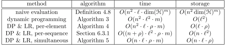
+. The results are summarized in Table 2. The key are the recursive Horner-type formula given in Corollary 4.9 together with ideas from dynamic programming and low-rank approximations.
method algorithm time storage
naive evaluation Definition 4.8 O(n2·`·dim(H)m) O(n2dim(H)m)
dynamic programming Algorithm 3 O(n2·`2·m) O(`2) DP & LR, per-element Algorithm 4 O(n2·`·ρ·m) O(`·ρ) DP & LR, per-sequence Section 6.3.1 O((n+ρ)·`2·ρ·m) O(n·`2) DP & LR, simultaneous Algorithm 5 O(n·`·ρ·m) O(n·`·ρ)
Table 2: Computational time (in elementary arithmetic operations) and storage cost for computing (an approximation) to the (n×n)-Gram matrix k+m(xi, xj)
i,j∈{1,...,n}
between sequences x1, . . . , xn ∈ X+ of length at most `, that is |xi| ≤ ` for i = 1, . . . , n. Methods: DP = dynamic programming, LR = low-rank. In the low-rank methods,ρ is a meta-parameter which controls accuracy of approximation.
Remark 6.1 Naive evaluation ofk+m(x, y) by directly calculating it as an inner product of signature features incurs an exponential storage cost O(dim(H)m). Even for H =Rd this
becomes quickly very expensive and infeasible when dim(H) =∞ which is the case for most practically relevant kernels.
Remark 6.2 Above algorithms are already powerful for H=Rd with the inner product in Rd as kernel k. In this case, k+x ≈ S(kx) = S(hkx,·i) 'S(x) ∈Qm≥0 Rd
⊗m
, that is the
feature map for a path x is the usual signature S(x) ∈Q
m≥0 Rd ⊗m
Remark 6.3 For readability we have absorbed in Table 2 the computational time c that is needed to evaluatek(x, y) forx, y∈Xinto the big O bound since this is just a multiplicative factor. E.g. the computational time for Algorithm 3 would readO(c·n2·`2·m) if we include c.
6.1. Notation and subroutines for computations with arrays (tensors)
We introduce notation (inspired by Python/Numpy) and fast algorithms for dynamic pro-gramming subroutines. This allows us to express our algorithms as operations on arrays alone and makes it easy to implement them in high-level languages that are optimized for operating on arrays (such as Numpy, etc).
Notation 6.4 (Arrays/tensors) We will denote the (i1, . . . , ik)-th element of a k-fold array (= degree k tensor) A by A[i1, . . . , ik]. Occasionally, for ease of reading, we will use “|” instead of “,” as a separator, for example A[i1, i2|i3, . . . , ik] if the indices on the left side of “|” are semantically distinct from those on the right side. The arrays all contain elements inR, and the indices will always be positive integers, excluding zero.
Notation 6.5 (functions applied elementwise) For a functionf :R→R, and an
ar-rayA, we will denote byf(A)the array wheref is applied element-wise. I.e.,f(A)[i1, . . . , ik] =
f(A[i1, . . . , ik]). Similarly, for f :Rm →Rand arrays A1, . . . , Am, we denote
f(A1, . . . , Am)[i1, . . . , ik] =f(A1[i1, . . . , ik], . . . , Am[i1, . . . , ik]).
For example, 12 ·A2 is the array A having all elements squared, then divided by two. The arrayA+B contains, element-wise, sums of elements of A andB.
Notation 6.6 (slice, shift, cumulative sum) LetA be ak-fold array of size(n1× · · · ×
nk).
(i) For an index ij (at j-th position), we will write A[:, . . . ,:, ij,:, . . . ,:] for (k−1)-fold array of size(n1× · · · ×nj−1×nj+1×. . . nk) such that
A[:, . . . ,:, ij,:, . . . ,:][i1, . . . , ij−1, ij+1, . . . , ik] =A[i1, . . . , ik].
We define in analogy, iteratively, A[:, . . . ,:, ij,:, . . . ,:, ij0,:, . . . ,:], and so on. Arrays of this type are called slices (ofA).
(ii) For an integer m, we will write A[:, . . . ,:,+m,:, . . . ,:] for the k-fold array of size (n1× · · · ×nj−1×(nj+m)×nj+1× · · · ×nk) such that
A[:, . . . ,:, ij,:, . . . ,:][i1, . . . , ij−1, ij+m, ij+1, . . . , ik] =A[i1, . . . , ik],
(iii) We will write A[:, . . . ,:,,:, . . . ,:], whereis at thej-th position, for thek-fold array of size (n1× · · · ×nk) such that
A[:, . . . ,:,,:, . . . ,:][i1, . . . , ik] = nj
X κ=ij
A[i1, . . . , ij−1, κ, ij+1, . . . , ik].
Arrays of this type are called slice-wise cumulative sums (of A).
(iv) We will write A[:, . . . ,:,Σ,:, . . . ,:], where Σ is at the j-th position, for the (k− 1)-fold array of size (n1 × · · · ×nj−1×nj+1 × · · · ×nk) such that A[:, . . . ,:,Σ,:, . . . ,: ][i1, . . . , ik−1] =
Pnj
κ=1A[i1, . . . , ij−1, κ, ij, . . . , ik−1].Arrays of this type are called slice-wise sums (of A).
We will further use iterations and mixtures of the above notation, noting that the index-wise sub-setting, shifting, and accumulation commute with each other. Therefore expressions such as A[+1,:|Σ,+2] or A[j|:,+3,] are well-defined, for example. We will also use the notation A[+m, . . .] to indicate the shifted variant of the cumulative sum array.
Cumulative sums can be computed efficiently, in the order of the size of an array, as opposed to squared complexity of more naive approaches. The algorithm is classical, we present it for the convenience of the reader in Algorithms 1 and 2.
Algorithm 1 Computing the cumulative sum of a vector. Input: A 1-fold array A of size (n)
Output: The cumulative sum arrayA[] 1: LetQ←A.
2: for κ= 2 to ndo
3: Q[κ]←Q[κ−1] +A[κ]
4: end for 5: Return Q
Algorithm 2 Computing the cumulative sum of an array. Input: A k-fold array Aof size (n1× · · · ×nk)
Output: The cumulative sum arrayA[, . . . ,,:, . . . ,:] (up to them-th index) 1: LetQ←A
2: for κ= 2 to mdo
3: Let Q←Q[:, . . . ,:,,:, . . . ,:] (at the κ-th index), where the right side is computed via applying algorithm 1 slice-wise.
6.2. Computing the discretized signature kernel
Algorithm 3 Evaluation of k+m.
Input: Sequences x, y∈X+. A kernel k :X×X→
R. A truncation degreem.
Output: k+m(x, y)
1: Set`x=|x| −1, `y =|y| −1
2: Compute the (`x×`y)-array K with entries K[i, j] =∇i,jk(x, y) 3: Initialize an (m×`x×`y)-array A
4: SetA[1|:,:]←K
5: for d= 2 to mdo
6: Compute Q←A[d−1|,]
7: Set A[d|:,:]←K·(1 +Q[+1,+1]) 8: end for
9: Compute R←1 +A[m|Σ,Σ]
10: Return R
The correctness of above Algorithm follows directly from the recursive formula (3) in Corol-lary 4.9: we start by evaluating the innermost parenthesis and then use the summation to build the content of the next parenthesis. In symbols, define ford= 1, . . . , m−1 ,
A1i,j :=∇i,jk(x, y) andAd+1i,j :=∇i,jk(x, y)
1 +X i0>i j0>j
Adi0,j0
,
then k+m(x, y) = 1 +P i≥1 j≥1
Ami0,j0. In above Algorithm 3 we denote A[d|i, j] =Adi,j.
Remark 6.7
• Disregarding the cost of computing the (`x ×`y)-matrix (∇i,jk(x, y))i,j, the compu-tational cost of Algorithm 3 is O(m|x||y|) elementary arithmetic operations (= the number of loop elements) and O(m|x||y|) units of elementary storage. The storage requirement can be reduced toO(|x||y|) by discardingA[d−1|:,:] from memory after step 7 each time.
• In each run of the loop, a matrixQis pre-computed to avoid a five-fold loop that would be necessary with the more naive version of line 7,
A[m|i, j]←A[m|i, j]·
1 +
X i0>i
X j0>j
A[m−1|i0, j0] ,
6.3. Large scale strategies
By using Algorithm 3 one can compute the Gram matrix k+m(xi, xj)
i,j=1,...,nofnsequences
x1, . . . , xn∈X+inO(n2·`2·m) elementary arithmetic operations. While this is for moderate sizes of n,m and ` achievable on contemporary desktop computers, it becomes quickly prohibitive for large n, ` due to the quadratic growth — especially when combined with parameter tuning or cross-validation schemes (as later in our experiments). We present two low-rank techniques to address this: the first is classic and reduces the quadratic cost inn to linear, the second reduces the quadratic cost in ` to linear. Finally, we combine these two techniques to get O(n·`·m·ρ) computation time withρ denoting an approximation parameter.
6.3.1. Low-rank methods for the sequence-vs-sequence kernel matrix
Since k+m(xi, xj)
i,j=1,...,n is a Gram-matrix, it is directly amenable to large-scale variants of low-rank type. Strategies of this kind include the incomplete Cholesky decomposition, Nystr¨om approximation, or the inducing point formalism in a Gaussian process framework. For n sequences, all strategies mentioned above require evaluation of at most an (n×r) and an (r×r) matrix (where r is a meta-parameter), which costs O((r+n)·r ·`2·m) elementary operations and O((r+n)·r·`2) storage11. Any of these low-rank strategies reduces the complexity of the Gram matrix to be linear inn, but not in`since the strategy is completely independent of how the discretized signature kernel was evaluated at a given pair (xi, xj)∈X+×X+. For the same reason, any improvements on the cost of evaluating k+m(xi, xj) will combine with this strategy.
6.3.2. Low-rank methods for the element-vs-element kernel matrix
The evaluation k+m(xi, xj) for a pair (xi, xj) ∈ X+ is given by nested partial summations and multiplications applied to the (`j × `j)-matrix (k(xi,r, xj,s))r,s where r = 1, . . . , `i,
s= 1, . . . , `j and we denote xi = (xi,1, . . . , xi,`i), xj = (xj,1, . . . , xj,`j)∈ X
+. The low-rank methods of the previous paragraph cannot be applied naively to this (`i×`j)- matrix: firstly, this matrix is in general non-symmetric; secondly, the summation- and multiplication-type operations require in naive form at each recursion step access to the full (`i ×`j)-matrix. The first issue is easily addressed by replacing the respective symmetric decomposition with the analogous non-symmetric one. The second issue is much harder to deal with, but below we show that by working exclusively on low-rank factorizations in each recursion step this issue can also be dealt with.
Definition 6.8 LetAbe an(a×b)-matrix. ForU an(a×r)-matrix, andV a(b×r)-matrix, we say that (U, V) is a low-rank presentation of A, of rank r, if
Ai,j = r X r0=1
Ui,r0Vj,r0
With • denoting the usual matrix multiplication this is equivalent to A=U •V>.
The fact that Ahas a low-rank presentation of rankr does imply thatA is of rankr or less (by equivalence of matrix rank with decomposition rank), but it does not imply thatA is of rank exactlyr.
We state a number of straightforward but computationally useful Lemmas that show how low-rank matrices behave under shifting, summation and cumulative summation, component-wise addition and multiplication. This allows us to replace these operations on matrices in Algorithm 4 by the operations on low-rank matrices.
Lemma 6.9 (Low-rank under cumulative summations and shifts) Let (U, V) be a low-rank representation of rank r for an(a×b)-matrixA. Then
(i) Define A0 and A00 as A0i,j = P
i0≥iAi0,j and A00 i,j =
P
j0≥jAi,j0. Define U0 as U0 i,r = P
i0≥iUi0,r andV0 as V0 j,r =
P
j0≥jVj0,r. Then (U0, V) is a low-rank representation or rank r of A0 of rank and (U, V0) is a low-rank representation of rank r of A0.
(ii) Define A0 and A00 as A0i,j =Ai+s,j and A00i,j =Ai,j+s for s≥1. Define U0 and V0 as
Ui,r0 =Ui+s,r1i+s≤aandVj,r0 =Vj+s,r1j+s≤b. Then(U0, V)is a low-rank representation of A0 of rank r and (U, V0) is a low rank representation of rankr of A00.
Proof This follows by spelling out the definition: for (i)
A0i,j =X i0≥i
Ai0,j = X i0≥i
r X r0=1
Ui0,r0Vj,r0 = r X r0=1
Ui,r0 0Vj,r0;
for (ii)
A0i,j =Ai+s,j= r X r0=1
Ui+s,r0Vj,r0 = r X r0=1
Ui,r0 0Vj,r0.
The statements forA00 follow similarly.
Lemma 6.10 (Low rank under addition and multiplication) Let A1, A2 be (a×b )-matrices such that (U, V) is a low-rank representation of A1 of rank r1, and (R, S) is a low-rank representation of A2 of rank r2. Then
(i) (U0, V0) is a low rank representation of A1+A2 of rank r1+r2 where
Ui,r0 = (
Ui,r , if 1≤r ≤r1
Ri,r−r1 , if 1 +r1≤r≤r1+r2
, Vj,r0 = (
Vj,r , if 1≤r≤r1
Sj,r−r1 , if 1 +r1 ≤r≤r1+r2
(ii) ( ¯U ,V¯) is a low rank representation of12 A1◦A2 of rank r1r2 where ¯
Ui,r=Ui,aRi,b and V¯j,r =Vj,aSj,b
ProofSince the (i, j)-entry of the matrixA1+A2 equalsPrr=11 Ui,rVj,r+Prr20=1Ri,r0Sj,r0 and the (i, j)-entry ofA1◦A2 equalsPrr=11 Ui,rVj,rPrr20=1Ri,r0Sj,r0, the result follows by substi-tuting the two sums overr ∈ {1, . . . , r1}andr0 ∈ {1, . . . , r2}by one sum over{1, . . . , r1+r2} resp. over{1, . . . , r1r2}.
In view of Point (ii) of above Lemma we introduce new array notation:
Notation 6.11 Let A1 be ak-fold array of size (n1× · · · ×nk)and A2 be ak-fold array of size (n1× · · · ×nk−1×n0k). Write A1? A2 for the(n1× · · · ×nk−1×(nk·n0k)) array with entries
A1? A2[i1, . . . , ik] =A1[i1, . . . , ik−1, a]A2[i1, . . . , ik−1, b]
where a, b are such thatik= (a−1)·n2+b−1 with a∈ {1, . . . , n1} and b∈ {1, . . . , n2}.
Algorithm 4 Evaluation of k+m, with low-rank speed-up. Input: Sequences x, y ∈ X+. A kernel k : X×X →
R. A truncation degree m ≥ 1. An
integer 1≤r ≤min(`x, `y).
Output: An approximation to k+m(x, y) 1: Set`x← |x| −1 and`y ← |y| −1
2: Compute a low-rank representation (U, V) of rank r, approximating the element-vs-element matrix/array with entries K[i, j] =∇i,jk(x, y), i∈ {1, . . . , `x},j∈ {1, . . . , `y} 3: Initialize an (m×`x× ∗)-arrayB and an (m×`y× ∗)-array C (* means that the size
may change dynamically)
4: SetB[1|:,:]←U and C[1|:,:]←V
5: for d= 2 to mdo
6: P ←B[d−1|+1,:] andQ←C[d−1|+1,:]
7: Append an (`x×1)-array of 1’s toP and append an (`y×1)-array of 1’s toQ 8: Set B[d|:,:]←(U ? P)[:,:] andC[d|:,:]←(V ? Q)[:,:]
9: optional: “simplify” the low-rank presentation (B, C), reducing its rank 10: end for
11: SetR←B[m|Σ,:] andS ←C[m|Σ,:] 12: Return 1 + (R·S)[Σ]
Algorithm 4 first approximates the element-vs-element (`x×`y)-matrixK= (∇i,jk(x, y))i,j by a low rank approximation (U, V). It then uses the formula for k+m given in Corollary 4.9 and updates the low-rank representation in each recursion step (starting from the innermost parenthesis):
• The first time line 6 is called it uses Lemma 6.9 to calculate a low-rank
represen-tation (P, Q) of the (`x ×`y)-matrix
P
i0>i,j0>j∇i0,j0k(x, y)
• The first time line 7 is called, it calculates a low-rank representation ( ¯P ,Q¯) of the (`x×`y)-matrix (1 + (P •Q>)i,j)i,j by using (P, Q) and the trivial identity
1 + r X k=1
Pi,kQj,k = r+1 X k=1
¯ Pi,kQ¯j,k
where ¯P and ¯Q are given by adding a (r+ 1)-th column consisting of 1’s. Note that the rank increases by one by going from (P, Q) to ( ¯P ,Q¯). Later calls do the same but with (P, Q) replaced by another matrix with low-rank factorization stored in B[d|:,:] and C[d|:,:].
• Line 8 calculates a low-rank representation ( ¯U ,V¯) for the elementwise product between the (`x ×`y)-matrices K = U • V> and ¯P • Q¯>. By Lemma 6.10 it is given as
¯
Ui,¯r=Ui,aP¯i,b and ¯Vr,j¯ =Va,jQ¯b,j.
• Line 9 is optional, aiming at keeping the low-rank presentation small13.
• Line 11 uses that
X i≥1,j≥1
(R•S>)i,j = X i≥1,j≥1
X k
Ri,kSj,k = X
k (X
i≥1
Ri,k)( X j≥1
Sj,k).
(Recall thatR·S denotes elementwise multiplication of arraysR, SandR•Sdenotes the usual matrix multiplication ifR, S are interpreted as matrices).
• The computational cost of Algorithm 4 is of the same order as the maximum size of B and C. That is, if ρ is the smallest integer such that at any time B requires `x·m·ρ space, andC requires `y·m·ρspace, then the computational complexity of Algorithm 4 is14 O((`x+`y)·ρ·m).
6.3.3. Simultaneous low-rank methods
Algorithm 4 yields an efficient low-rank speed-up for computing a single entry k+m(xi, xj). Thus total computational cost for the Gram matrix (k+m(xi, xj))i,j∈{1,...,n} isO(n2·`·ρ·m)
and cost quadratic in the number of data points nmay be prohibitive on large scale data. We address this by combining both low-rank strategies mentioned before to achieve a further reduction of computational cost fromO(n2·`·ρ·m) to O(n·`·ρ·m).
13. This can be achieved for example via singular value decomposition, sub-sampling, or random projection type techniques.
14. Since one can always choose a low-rank representation ofB[m|:,:] andC[m|:,:] of rank min(`x, `y) or
Algorithm 5 Computation of the Gram matrix of k+m, with (double) low-rank speed-up. Input: Sequences x1, . . . , xn ∈ X+. A kernel k : X×X→ R. A truncation degree m. An
integerr ≥1.
Output: A low-rank approximation (U, U) of the Gram matrixK = k+m(xi, xj)
i,j=1,...,n.
1: Compute arrays U(i) such that each pair (U(i), U(j)) i, j ∈ {1, . . . , n} is a low-rank presentation of rankr for the ((|xi| −1)×(|xj| −1))-matrixK(ij) with entries Ka,b(ij)=
∇a,bk(xi, xj)
2: Initialize an (n×m× ∗ × ∗)-arrayB (where * means that the sizes may change dynam-ically)
3: B[i|1|:,:]←U(i) for all i∈ {1, . . . , n}
4: for d= 2 to mdo
5: Compute P ←B[:|d−1|+1,:]
6: Set κ, ρsuch that (n×κ×ρ) is the size ofP
7: Append an (n×κ×1)-array of ones toP
8: B[:|d|:,:]←B[:|1|:,:]? P[:,:,:]
9: optional: “simplify” the low-rank presentation encoded in B, reducing its rank 10: end for
11: Compute U ←B[:|m|Σ,:]
12: Return U
Algorithm 5 is obtained as follows:
• The previous Algorithm 4 transforms for any pairxi, xj ∈X+ a low rank representa-tion (U(ij), V(ij)) of the (`
i×`j)-matrix K(ij) = (∇a,bk(xi,a, xj,b))a,b into a low-rank representation (R(ij), S(ij)) such that
k+(xi, xj) = 1 + X a≥1,b≥1
R(ij)•(S(ij))>
a,b.
But if U(ij) is independent of j and if V(ij) is independent i, then R(ij) will depend by Algorithm 4 only on iand S(ij) will depend only on j; hence R(ij) =S(ji). If we denoteR(i):=R(ij):=S(ji), then in above Algorithm 5,B[i, m, a, r] equalsR(i)a,r when the end of the for loop is reached, line 10.
• Write
k+m(xi, xj) = 1 + X a≥1 b≥1
R(i)•(R(j))>
a,b= 1 + r0 X k=1
X a≥1
R(i)a,kX
b≥1
R(j)b,k
= r0+1 X k=1
¯ Ri,kR¯j,k
where we denote withr0 the rank of (R(i), R(j)) and set ¯Ri,k :=Pa≥1R (i)
Remark 6.12 Line 1 requires that for each pair of sequences xi = (xi,a)a=1,...,`i, xj =
(xj,b)b=1,...,`j ∈ X
+ we compute the (`
i×`j)-matrix K(ij) with entries Ka,b(ij) = k(xi,a, xj,b). That is, the matricesU(i), when row-concatenated, should have low rank15. Jointly low-rank
U(i) can be obtained by running a suitable joint diagonalization or singular value decompo-sition scheme on the matrices K(ij).
Remark 6.13 (Fast sequential kernel methods) By Section 5, fast string kernel meth-ods such as the gappy, substitution, or mismatch kernels presented in Leslie and Kuang (2004) may be transferred to general sequential kernels. In general, this amounts to small modification of Algorithm 3; for example, to obtain a gappy variant of the sequential kernel, summation in line 6 of Algorithm 3 over the whole matrix, of quadratic size, is replaced by summation over a linear part of it.
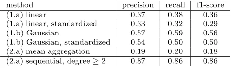
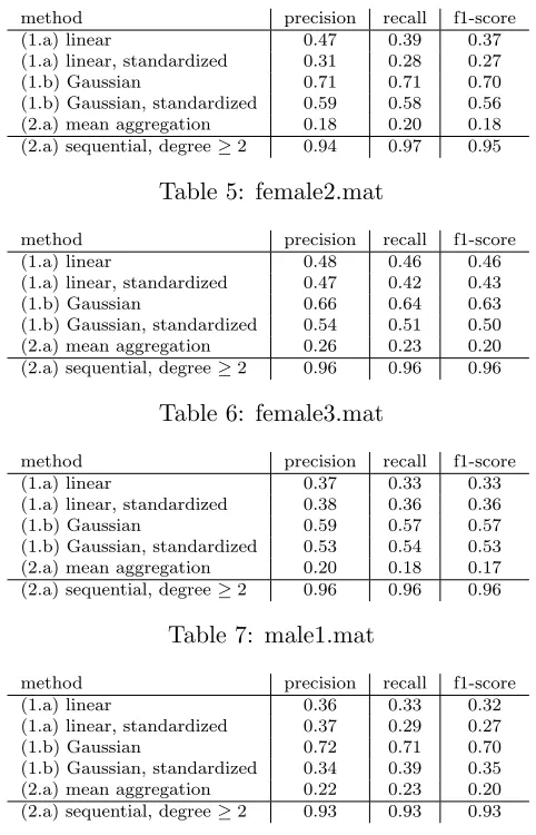
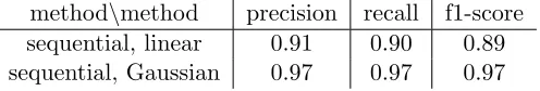
7. Experimental validation
We perform two experiments to validate the practical usefulness of the signature kernels:
(1) On a real world data set of hand movement classification (eponymous UCI data set Sapsanis et al. (2013)), we show the discretized signature kernel outperforms the best previously reported predictive performance Sapsanis et al. (2013), as well as non-sequential kernel and aggregate baselines.
(2) On a real world data set on hand written digit recognition (pendigits), we show that the discretized signature kernel over the Euclidean kernel (= linear use of signature features) achieves only sub-baseline performance. Using the discretized signature kernel over a Gaussian kernel improves prediction accuracy to the baseline region.
We emphasize that our experiments do not constitute a systematic benchmark com-parison to prior work, only validation that the signature kernel is a practically meaningful concept: experiment (1), shows that the sequentialization of standard kernels can achieve state-of-the-art performance on time series data; experiment (2) shows that even for paths in low dimensions, X = R2, using a non-linear static kernel for the sequentialization
out-performs the linear kernel (the latter corresponds to learning with signature features of a 2-dimensional path; the former, corresponds to learning with signature features of the path lifted to the RKHSH of the non-linear kernel).
A systematic benchmark comparison is likely to require a larger amount of work, since it would have to include a number of previous methods (multiple variants of the string and general alignment kernels, dynamic time warping, naive use of signatures), for most of which there is no freely available code with interface to a machine learning toolbox, and benchmark methods (order-agnostic baselines such as summary aggregation and chunking; distributional regression; naive baselines).