583
Copyright © 2011-15. Vandana Publications. All Rights Reserved.
Volume-5, Issue-2, April-2015
International Journal of Engineering and Management Research
Page Number: 583-589
International Reserves Accumulation and Economic Growth: Evidence
from India
Mohammad Kashif1, Dr. P. Sridharan2
1
Research Scholar, Department of International Business, School of Management, Pondicherry University, INDIA
2
ABSTRACT
The present study analyses empirically the impact of economic growth on international reserves in India. We employed time series data with annual frequency from 1993 to 2013. We develop an econometric model relating RES to ECON variables and used logarithmic transformation of the variables for econometric estimation. The econometric tools such as Augmented Dickey-Fuller (ADF) test, Johansen cointegration test and vector error correction model were applied. The cointegration test results suggest that there is an existence of a stable long-run equilibrium relationship between international reserves and economic growth. The VECM of international reserves reveals that lagged independent variables shows the expected signs i. e. economic growth have significant effect on international reserves. Findings of the study suggest that economic growth is positively related to international reserves. This implies that India has to involve more actively in foreign reserve management practices.
Keywords---- Economic growth, International reserves, VECM, Cointegration, India.
Associate Professor & Head, Department of International Business, School of Management, Pondicherry University, INDIA
I.
INTRODUCTION
Over the past few years, there has been a remarkable increase in International reserves with the central banks of developing economies around the world, especially in the aftermath of East Asian crisis 1997-98. Total world international reserves have climbed nearly from US$7.4 trillion in 2008 to US$12.3 trillion by March’2014. The management of these huge reserves and the associated cost of holding are the major issues faced by the central banks of developing economies now.
International Reserves, also called as foreign reserves and foreign exchange reserves, are foreign currencies and
deposits in the form of securities, bonds and financial derivatives held by Central Banks and monetary authorities of any economy. The components of IR comprises of monetary gold Special Drawing Rights and IMF reserves positions. International Reserves may also be referred to as official reserves which are assets of Central Banks held in different reserves currencies such as US Dollar, British Pound Sterling, Euro and Japanese Yen (Reza et al. 2011). According to IMF Balance of Payments Manual 6th
Over the last decade, the pace of accretion in the India’s stock of international reserve has been so striking that it has registered more than 1000% growth, despite the fact that India has entered into flexible exchange rate system since March 1993(Ramachandran, 2006). And now it seems convincing to believe that India has surpassed many standard measures of reserve adequacy to rest in a somewhat protected zone. Theoretically, it was believed that under flexible exchange rate system countries will need to keep less stock of international reserves, since edition (BPM6), reserve assets (gross international reserves) are those “external assets that are readily available to and controlled by the monetary authorities for meeting balance of payments financing needs, for intervention in exchange rate markets to affect the currency exchange rate, and for other related purposes (such as maintaining confidence in the currency and the economy, and serving as a basis for
foreign borrowing).”
584
Copyright © 2011-15. Vandana Publications. All Rights Reserved.
central banks were not obligated to defend their parities through frequent interventions.
India’s stock of international reserves has been increasing continuously since the launch of economic reform in 1991. Starting from a stumpy level of US$ 5,834 million in 1990-91, the stock of international reserves increased regularly to US$ 1,99,179 million by 2006-07 and reached their highest at US$ 3,04,818 million in 2010-11 (see figure 1). Thereafter, owing the international financial disorder caused by 2008 crisis and strengthening of the US dollar and other international currencies, the stock of reserve declined to US$ 2, 51, 985 million at the end of 2008 and again touched the height of US$ 3, 04, 223 million by 2013-14. This evidently shows that irrespective of all the theoretical justifications, international reserves stock of India like many emerging countries has been constantly increasing during the economic reform period i. e.1991-till date.
Figure1: India’s international reserves in the post reform era
Source: handbook of statistics on Indian economy
After this introduction, rest of the paper is organised as: Section II discusses relevant review of literature, section III discusses objectives of the study whereas section IV presents data description and methodology, section V discusses about results and interpretations and section VI concludes.
II.
REVIEW OF LITERATURE
Conceptually, a unique definition of foreign reserves is not available as there have been divergence of views in terms of coverage of items, ownership of assets, liquidity aspects and need for a distinction between owned and non-owned reserves. Nevertheless, for policy and operational purposes, most countries have adopted the definition suggested by the International Monetary Fund
(Balance of Payments Manual, and Guidelines on Foreign Exchange Reserve Management, 2001); Which defines reserves as external assets that are readily available to and controlled by monetary authorities for direct financing of external payments imbalances, for indirectly regulating the magnitudes of such imbalances through intervention in exchange markets to affect the currency exchange rate, and/or for other purposes.
According to Krugman and Obstfeld, Official international reserves (or foreign exchange reserves) are assets held by central banks of respective economies that are used for various transactions such as purchases of foreign goods and assets, or payments of obligations to international organisations.
Foreign exchange reserves are defined as external stock of assets, which is available to the country’s monetary authorities to cover external payment imbalances or to influence the exchange rate of the domestic currency through intervention in exchange market, or for other purposes (IMF, 2000). A country’s reserve consists of gold, foreign currencies, special drawing rights (SDR) and the reserve position with the International Monetary Fund (IMF).
Historically, official international reserves consisted only of gold. But after World War II when the Breton Woods System was set up, the US Dollar turn out to be reserve currency and it also became part of a nation’s official IR assets. From 1944-1968, the US dollar was convertible into gold through the Federal Reserve System. After 1968 no central bank could convert dollars to gold from official gold reserves and after 1973 no individual or institution could convert dollars into gold from official gold reserves. Since 1973 no major currencies have been convertible into gold from official gold reserves.
Under the Bretton-Woods system, the foreign exchange reserves were used by the central banks across the world to maintain the external value of their respective currencies at a fixed level. With the breakdown of Bretton-Woods system in the early 1970s, countries started adopting a relatively flexible exchange rate system, under which the reserves play only a less important role. Yet, the global exchange reserves have increased from1.75 to 7.8 percent of world GDP between1960 and 2002 (Flood and Marion, 2002).
The following specification from Aizenman and Lee’s (2007) can be used to investigate factors influencing international reserves-
Re Sit = β0+ β1EXGrowthit+ β2PLDevit-1 + β3KAccit+ β4Debtit
+ β5Popit+ β6Openit+β7TOTit+ ε
Where, EXGrowth, PLDev, KAcc, Debt,Pop, Open, TOT denotes higher export growth rates, Price Level Deviation, capital account liberalization, log of the ratio of short-term external debt to Gross Domestic
it 0
50000 100000 150000 200000 250000 300000 350000
1991 1996 2000 2005 2008 2009 2010 2014
M
illio
n U
S$
Year
585
Copyright © 2011-15. Vandana Publications. All Rights Reserved.
Product, Population size, log of ratio of imports to GDP, log of the terms of trade respectively.
Several conclusions emerge from the specification. First, the holding of foreign reserves motivated by mercantilist concerns is positively correlated with higher export growth rates (variable EXGrowthit) and
with the deviation of the real exchange rate from its equilibrium value (Price Level Deviation noted PLDevit).
The latter observation captures the idea that international reserves are hoarded to manipulate the exchange rate.
Second, the holding of reserves motivated by precautionary concerns is positively correlated with the degree of capital account liberalization (KAccit) and the
log of the ratio of short-term external debt to Gross Domestic Product (GDP) (Debtit).
Third, the reserves stock is positively correlated with a country’s population because reserves increase as the number of international transactions increases. In addition, reserves accumulation is positively correlated with the log of ratio of imports to GDP (Openit). Last, the
log of the terms of trade (ToTit
Gosselin and Nicolas (2005) grouped the influencing factors of reserve holdings in five categories: economic size, current account vulnerability, capital account vulnerability, exchange rate flexibility, and opportunity cost. In the long run, central banks will increase their reserves in response to a greater exposure to external shocks. Thus, the level of foreign reserves could
be positively correlated with an increase in both exports and imports. Capital account vulnerability increases with financial openness and potential for resident-based capital flight from the domestic currency. Consequently, reserves could be positively correlated with some variables like the ratio of capital flows to GDP. Exchange rate flexibility is usually important.
Charles (2012), in his study finds the factors that affect the level of foreign reserves are GDP, level of trade openness, exchange rate and inflation. The levels of GDP and trade openness were found to exhibit positive impacts on foreign reserves, supporting the self-insurance theoretical base of foreign reserves. Whereas the level of foreign capital inflow and inflation had a negative relationship with foreign reserves.
India Economic Survey (2004) identified three main factors that predicated the nation’s reserve holdings which include: import adequacy—the number of months of imports that it can finance; its ability to cover external payment obligations—captured by the ratio of reserve to external and short-term debt; and monetary adequacy— measured by ratio of reserve to broad money and reserve money. Demand for liquidity is one of the factors influencing international reserves.
III. OBJECTIVES OF THE STUDY
Almost all economies particularly developing countries have accumulated large stockpiles of international reserves on breakdown of the Bretton Wood system. They reflect fabulous increase in international reserves. The flexible exchange rate system was introduced after breakdown of Bretton Wood System. Henceforth, developing countries have frightened the uncertainties of this system. They embarked accumulating international reserves to intervene FX markets to get price stability and lessen foreign exchange volatility. The hoarding of these reserves is made irrespective of the opportunity cost and the effects they have on price stability and volatility. Another reason to have large stockpile of international reserves is foreign debt service and international trade activities. The import and export transactions affect foreign exchange reserves as foreign currencies get involved in these transactions. The more export of goods and services will fetch more economic growth. This paper, therefore, assesses how international reserves affect economic growth.
) is positively correlated with reserves if countries absorb their fluctuations through reserves holdings.
Frenkel and Jovanovic (1981) states that most of the rules for a country’s demand for foreign exchange reserves consider real variables, such as imports, exports, foreign debt, severity of possible trade shocks and monetary policy considerations. Similarly, Shcherbakov (2002) states that, there are some common indicators that are used to determine international reserves for an economy. These indicators includes: import adequacy, debt adequacy and monetary adequacy.
Chin-Hong et al. (2011) empirically examined five explanatory variables to investigate their impacts on the international reserves holding in Malaysia. These variables include economic size, real effective exchange rate, openness, balance of payments and the opportunity cost of reserves holding. They concluded that all the variables are found to be statistically significant in the model. In particular, economic size and real effective exchange rate are positively related to international reserves, while balance of payments and the opportunity cost of holding reserves have negative impacts on international reserves.
Empirical research works on foreign reserves (e.g. Landell-Mills, 1989; Lane and Burke, 2001) established a relatively stable long-run demand for reserves based on a limited set of explanatory variables such as gross domestic
586
Copyright © 2011-15. Vandana Publications. All Rights Reserved.
suggests that high level of reserves is the outcome of countries' mercantilist behavior to keep their real exchange rate devalued against the dollar to bolster the domestic economy (Flood and Marion, 2001).
Countries all over the world in particular developing ones are fanatical with accumulation of international reserves. Several explanations as we have seen in earlier lines advocated for reserves hoarding. International reserves have both social and opportunity costs that impact the whole economy. A lot of studies are there on international reserves but not much appears to have been done to examine the effect on economic growth. This study contributes to international reserves literature by examining the effect that international reserveshave on economic growth in Indian context. Hence, this paper is toadd to existing knowledge. Also there will be some information on hoarding of international reserves and economic growth relationship. The findings will thus enrich the existing literature. The main aim of this study is to find why India hoard reserves. Other objective is to explore the influence thateconomic growth have on international reserves.
IV.
DATA DESCRIPTION AND
METHODOLOGY
The study employs secondary data and econometric modelling to obtain the results. Following is the data description and methodology applied:
(a) Data
The present study deals with extensive literature review which takes in the areas of international reserves and economic growth of India. Time series data for a period of 21 years from 1993 to 2013 were collected from World Development Indicators (WDI) of World Bank. The variables are arranged as dependent and independent variable. Dependent variable is international reserves (RES) measured as total reserves excluding gold divided by nominal GDP converted into logarithm form. Independent variable is economic growth (ECON)proxied by real GDP converted into logarithm form. E-Views package has been used to run regression equation.
(b) Model Specification
This study analyses the impact of international reserves on economic growth in Indian context. We develop an econometric model below relating RES to ECON variables and used logarithmic transformation of the variables for econometric estimation.
(RES) = β1+ β2
Where, (RES) is total international reserves minus gold divided by nominal GDP. (ECON) is economic growthproxied by the real GDP. β
(ECON)+ e ………(1)
1, and β2 are regression
coefficients for the model and e is an error term. Logarithmic transformation of the equation is as under:
Ln(RES) = β1 + β2
(c) Methodology
First we check for time series properties of the variables. We check stationarity of the series using Augmented Dickey-Fuller (ADF) test. If the variables are found to be order of I(1) or say non-stationary, there may be chances of forming I(0) variable. This is called cointegration which mean long-run relationship among the variables.The long-run relationship can be appropriately examined through cointegration tests. If the variables under study are cointegrated, the cointegrating vector is normalizedwith respect to international reserves. To test whether cointegration exists or not, we applythe systems method of cointegration proposed by Johansen and Juselius (1992).
The Johansen cointegration test suggests that variables are highly cointegratedindicating to employ vector error correction model (VECM).
Vector Error Correction Model (VECM)
If two I(1) series x and y are cointegrated, then
there exists unique α
Ln(ECON)+ e ……….(2)
0and α1 such that ut = yt - α0 - α1xt is
I(0). In the single equation model of cointegration where we thought of y as the dependent variable and x as an exogenous regressor, the appropriate specification for the error-correction model will be:
∆yt = β0 + β1∆xt + λu t-1 + εt ……….. (1)
Or,
∆yt=β0 + β1∆xt+ λ (yt-1-α0-α1xt-1) + εt …….. (2)
All terms in equation (2) are I(0) as long as the a coefficients (the “cointegrating vector”) are known or at least consistently estimated. The u t-1termis the magnitude
by which y was above or below its long-run equilibrium value in the previous period. The coefficient λ (which we expect to be negative) represents the amount of “correction”of this period-(t-1) disequilibrium that happens in period t. For example, if λ is 0.25, then one quarter of the gap between yt-1
The VEC model extends this single equation error correction model to allow y and x to evolve jointly over time as in a VAR system. In the two-variable case, there can be only one cointegrating relationship and the y equation of the VEC system is similar to (2), except that we mirror the VAR specification by putting lagged differences of y and x on the right hand side. With only
587
Copyright © 2011-15. Vandana Publications. All Rights Reserved.
one lagged difference (there can be more) the bivariate VECM can be written as:
∆yt = βy0 + βyy1∆yt-1 + βyx1∆xt-1 + λy(yt-1 -α0 -α1xt-1)
+ νty, …………. (3)
∆xt = βx0 + βxy1∆yt-1 + βxx1∆xt-1 + λx (yt-1 -α0 -α1xt-1)
+ νtx. ………….. (4)
As in (2), all of the terms in both equations (3) and (4) are I(0) if the variables are cointegrated with cointegrating vector (1, - α0 , - α1), in other words, if yt
-a0 - α1xt is stationary. The λ coefficients are again the
error correction coefficients, measuring the response of each variable to the degree of deviation from long-run equilibrium in the previous period.
We expect λy< 0 for the same reason as above: if yt -1is above its long-run value in relation to xt-1then the
error correction term in parentheses is positive and this should lead, other things constant, to downward movement in y in period t. The expected sign of λxdepends on thesign
of α1. We expect ∂∆xt / ∂xt-1 = - λx α1< 0 for the same
reason that we expect ∂∆yt / ∂∆yt-1 = λy< 0 : if xt-1 is
above its long run relation to y, then we expect, ceteris paribas, ∆xtto be negative.
A simple, concrete example may help clarify the role of the error correction terms in a VEC model. Let the long-run cointegrating relationship be yt= xt, so that α0 = 0 and α1 = -1. The parenthetical error correction term in equations of (3) and (4) is now yt-1 - xt-1, the difference
between y and x in the previous period. Suppose that because of previous shocks,yt-1 = xt-1 + 1 so that y is above
its long-run equilibrium relationship to x by one unit (or, equivalently, x is below its long-run equilibrium relationship to y by one unit). To move toward long-run equilibrium in period t, we expect (if there are no other changes) ∆yt < 0 and ∆xt > 0. Using equations (3) and (4) ∆yt changes in response to this equilibrium by λy (yt-1 - x t-1) = λy so for stable adjustment to occur λy < 0; y is “too
high” so it must decrease in response to the disequilibrium. The corresponding change in ∆xtfrom both equations is λx
(yt-1 - xt-1) = λx. Since x is “too low,” stable adjustment
requires that the response in x be positive, so we need λx > 0. Note that if the long-run relationship between y and x
were inverse (α1 < 0), then x would need to decrease in order to move toward equilibrium and we would need λx < 0. The expected sign on λx depends on the sign of α1.
If theory tells us the coefficients α0and α1
V.
RESULTS AND INTERPRETATION
of the cointegrating relationship,then we can calculate the error-correction term in both the equations and estimateit asastandardVAR.However,weusually do not know these coefficients, so they must be estimated.
To test the stationarity the widely applied Augmented Dickey-Fuller (ADF)unit root test has been used.All the variables i.e. international reserves (RES) and economic growth (ECON) was non-stationary at level. After first differencing, the variable become stationary i. e. order of I(1) (Table 1). This suggests there exists long-run relationship among the variables.
Table 1: Unit Root Testing (Augmented Dickey Fuller test)
Variables Level First Differenced
RES -1.092974 -4.720630* ECON -0.190311 -3.616661*
*denotes rejection of null hypotheses at 1% level
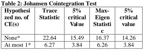
The long-run relationship can be appropriately examined through cointegration tests. For the purpose we employJohansen cointegration test. The significant values or trace statistics, maximal eigen value and critical values are given in table 2.
Table 2: Johansen Cointegration Test Hypothesi
zed no. of CE(s)
Trace Statistic
5% critical
Val ue
Max-Eigen Statisti
c
5% critical
value
None* 22.64 15.49 16.37 14.26 At most 1* 6.27 3.84 6.26 3.84
*denotes rejection of null hypotheses at 5% level
The normalized cointegrating coefficients imply theoretically expected signs and the standard errors in the parentheses indicate that the explanatory variables are statistically significant at 5 percent level. Thenormalized cointegrating coefficients are given in table 3.
Table 3: Normalized cointegrating coefficients
RES ECON
Normalized β 1.000 1.148 (0.121)*
*denotes significant at 5% level; Figures in parenthesis are standard error
Now, the long run equation of cointegration can be written as:
RES = 1.148 (ECON) ……….. (5)
The normalized equation of cointegration shows theoretically expected signs. The equation (5) suggests that a one percent increase in economic growth will lead more than one percent upsurge of international reserves.
588
Copyright © 2011-15. Vandana Publications. All Rights Reserved.
The variables ∆(ECON)and ∆(ECON) t-1
Variables
are found significant in vector error correction model.The determination coefficient R-squared is 60%. This means that changes in economic growth explains 60% of the reasons for India’s accumulation of international reserves over the years. Moreover the t-statistics is 4.36 with a p-value of 0.01. The t-stat result is used to test the hypothesis that- economic growthhave no significant effect oninternational reserves. Since the p-value is highly significant, the null hypothesis can be rejected and alternative hypothesis can be accepted. Therefore, economic growthhave significant effect on international reserves.
Table 5: Vector Error Correction Model (VECM) ∆(RES) ∆(ECON)
∆(RES) 0.385 (1.160)
t-1 -0.421
(-2.686)*
∆(ECON) -0.578 (-1.349)*
t-1 -0.204
(-1.011)
∆(RES) 0.016 (0.080)
t-2 -0.186
(-1.925)*
∆(ECON) -0.119 (-0.251)
t-2 -0.315
(-1.400) Constant 0.107
(1.242)
0.178 (4.364)* R-squared 0.35 0.60 F-Statistics 1.32 3.71 Std. Error 0.12 0.05
Note:Figures in parenthesis are t-statistics; * denotes significant at 5% level
Figure 2: Impulse responses of the variables
-.05 .00 .05 .10 .15 .20 .25
1 2 3 4 5 6 7 8 9 10
Response of RES to RES
-.05 .00 .05 .10 .15 .20 .25
1 2 3 4 5 6 7 8 9 10
Response of RES to ECON
-.04 .00 .04 .08 .12 .16
1 2 3 4 5 6 7 8 9 10
Response of ECON to RES
-.04 .00 .04 .08 .12 .16
1 2 3 4 5 6 7 8 9 10
Response of ECON to ECON
Response to Cholesky One S.D. Innovations
VI. CONCLUSION
This paper has analysed empiricallythe influence of economic growth on international reserves in Indian context. We employed time series data with annual frequency from 1993 to 2013. We develop an econometric model relating RES to ECON variables and used logarithmic transformation of the variables for econometric estimation. Our study agrees with Puah C. et al. (2011) in which they found economic size and real effective exchange rate positively related to international reserves in case of Malaysia.
The purpose of this study is to investigate empirically the effect of economic growth on international reservesin India. The ADF unit root test results indicate that all the variables are integrated with order one. Thus, we proceed to the Johansen-Juseliuscointegration test to study the long-run equilibrium associationship between the variables. The cointegration test results suggest that there is an existence of a stable long-run equilibriumrelationship between international reserves and economic growth at 5 % level of significance. By normalizing the cointegrating vector with respects to international reserves, we obtain the parameters that showing the relationship between economic growth and international reserves. The determination coefficient R-squared is 60%. This means that changes in economic growth explains 60% of the reasons for India’s accumulation of international reserves over the years. Moreover the t-statistics is 4.36 with a p-value of 0.01. The t-stat result is used to test the hypothesis that- economic growth have no significant effect on international reserves. Since the p-value is highly significant, the null hypothesis can be rejected and alternative hypothesis can be accepted. Therefore, economic growth have significant effect on international reserves. Findings of the study suggest that economic growth is positively related to international reserves. This implies that India has to involve more actively in foreign reserve management practices.
REFERENCES
[1] Aizenman, J., & Marion, N. (2003). The high demand for international reserves in the Far East: What is going
on? Journal of the Japanese and International Economics,
17, 370-400.
[2] Aizenman, Joshua, and Jaewoo Lee. 2007.
―International Reserves: Precautionary Versus
Mercantilist Views, Theory and Evidence, Open
Economies Review, Vol. 18, pp.191-214.
[3] Bahmani-Oskooee, M., & Brown, F. (2002). Demand for international reserves: a review article, Applied
Economics, 34, 1209-1226.
589
Copyright © 2011-15. Vandana Publications. All Rights Reserved.
Reserves in the Aftermath of Crises,” The World Economy, 26 (6): 873–891.
[5] Charles-AnyaoguNneka B (2012), External Reserves: Causality Effect of Macroeconomic Variables in Nigeria,
Kuwait Chapter of Arabian Journal of Business and Management Review Vol. 1, No.12; Aug 2012
[6] Dash P. and Narayanan K. (2011), “Determinants of Foreign Reserves in India: A Multivariate Cointegration Analysis”, Indian Economic Review, Vol. XXXXVI, No. 1 pp. 83-107.
[7] David A. and J. Halliday, The rationale for holding foreign currency reserves, RESERVE BANK OF NEW ZEALAND: Bulletin Vol. 61 No. 4
[8] Dooley et al. (2003), “An Essay on the Revived Bretton Woods System,” NBER Working Paper No. 9971 (Cambridge, MA: National Bureau of Economic Research).
[9] Edwards, Sebastian, 1983, ―The demand for international reserves and exchange rate adjustments: the case of LDCs, 1964–1972, Economica Vol. 50, pp. 269– 80.
[10] Garcia, P. and C. Soto, (2004): Large hoarding of international reserves: Are they worth it? Central Bank of
Chile Working Paper No 299.
[11] Gosselin M. A. and Nicolas P. (2005), An Empirical Analysis of Foreign Exchange Reserves in Emerging Asia, Bank of Canada Working Paper 2005-38 December 2005
[12] Heller, H. (1966), "Optional International Reserves" The Economic Journal, 76, 1966, pp. 296-311
[13] India Economic Survey (2004-05), accessed through
[14] Jeanne, O. and R. Rancière, 2006 ―The Optimal Level of Reserves for Emerging Markets: Formulas and Applications, IMF Working Paper 06/229. International Monetary Fund, Washington.
[15] Jeanne, Olivier and Romaine Ranciere, 2009, ―The Optimal level of International reserves for Emerging Market Countries: A New Formula and Some Applications, Working Paper, Johns Hopkins University. [16] Prabheesh K. et al. (2007), “Demand for Foreign Exchange Reserves in India: A Co-integration Approach”,
South Asian Journal of Management Vol.14, No.2, 2007, pp.36-46
[17] Prabheesh. K. et al. (2009), Modelling India’s Demand for International Reserves
[18] Puah, Chin-Hong et al. (2011), Determinants of international reserves in Malaysia, International Journal of Business Research, Volume: 11 Issue: 4, July, 2011 [19] Ramachandran, M. (2006). On the upsurge of foreign exchange reserves in India, Journal ofPolicy Modelling,
28, 797-809.
[20] Reza Mohaghadam, Johnson D. Ostry & Robert Sheehy (2011), Assessing Reserves Adequacy, International MonetaryFund, Prepared by Money and
Capital Markets, Research Strategy, Policy and Review Departments.
[21] Reserve Bank of India, Handbook of statistics on
Indian economy, RBI, Mumbai (various issues).
[22] Ritesh K. M.and Chandan S. (2010), the Demand for International Reserves and Monetary Equilibrium: New Evidence from India
[23] Rodrik, D. and A. Velasco, (1999): Short-Term Capital Flows, National Bureau of Economic Research,
Working Paper 7364, September 1999.