The Thirty-Third AAAI Conference on Artificial Intelligence (AAAI-19)
Cost-Sensitive Learning to Rank
Ryan McBride, Ke Wang
Simon Fraser University, BC, Canada[email protected] and [email protected]
Zhouyang Ren, Wenyuan Li
Chongqing University, Chongqing, China [email protected] and [email protected]Abstract
We formulate theCost-Sensitive Learning to Rankproblem of learning to prioritize limited resources to mitigate the most costly outcomes. We develop improved ranking models to solve this problem, as verified by experiments in diverse do-mains such as forest fire prevention, crime prevention, and preventing storm caused outages in electrical networks.
1. Introduction
Motivation
Learning to Rank originated in information retrieval (IR) and considers learning a ranking model for instances (such as documents, movies, or web pages) according to their rel-evance to a query. The training data is a list of pairs(x, y) for each query, withyas the instance’s relevance to the query (e.g., from zero, no relevance, to five, very relevant) andxas instance features. An effective ranking model aims to rank relevant instances correctly based onxfor a future query. Learning to Rank research thus primarily focuses on devis-ing more useful IR based metrics (Wang et al. 2016), im-proving performance on search engine data (Qin et al. 2010), or developing solutions in new IR fields (e.g., relevant image retrieval (Wang et al. 2014)).
However, we argue that many non-IR applications in in-dustry could benefit from similar ranking models: com-panies can learn to prioritize limited resources to events with a high y, the numeric cost/impact. One such prob-lem is with our industrial partner BC Hydro: storm caused power outages result in severe social peril and millions of dollars in economic losses every year (Insurance Journal 2017)(Bukaty 2013)(CBC News 2015)(Lawrence Berkeley National Laboratory 2004). A power company could rank potential outages for the next storm so high damage outages can be prevented. We define such problems as cost-sensitive ranking, problems of maximizing a company’s cost-saving via a ranking model:
Definition 1 (Cost-Sensitive Learning to Rank) Consider a training set of m “lists”, T = {Li}mi=1. The ith list
Li = (Xi, Yi) contains Xi = {xi,1,· · · , xi,ni} and
Yi = {yi,1,· · · , yi,ni}that describe the featuresxand the
Copyright c2019, Association for the Advancement of Artificial Intelligence (www.aaai.org). All rights reserved.
Figure 1: An example storm-caused power outage in Illi-nois from interactions between weather, cable placement, and surrounding vegetation. Ranking cities or geographical areas by their risk of large outages in the same storm is an example of our proposed Cost-Sensitive Ranking problem. Image credit to Wikipedia user Robert Lawton.
Figure 2: A training set consisting of instances of electricity supplying networks exposed to storms. Note that 1 m/s is approximately 2.2 miles per hour or 3.6 kilometres per hour.
Storm Electrical Cable Wind
Impact (Y)
ID Network In Length Speed
Storm1 City 1 5 km 14 m/s 10000 customers
Storm1 City 2 4 km 15 m/s 100 customers
Storm1 City 3 3 km 16 m/s 0 customers
Storm2 Rural 1 3 km 13 m/s 100 customers
Storm2 Rural 2 4 km 12 m/s 1 customer
Storm2 Rural 3 5 km 10 m/s 0 customers
cost/impact y of each instance in the list. The goal is to build a ranking model that can be used to rank future lists with instances that have knownxbut unknownyto mitigate damage or attain profit. Per the standard Learning to Rank assumptions, future lists are assumed sampled from the same underlying distribution asT (e.g., eachLi= (Xi, Yi)
is i.i.d. and(xi,j, yi,j)are also i.i.d. within eachLi).
cor-responding to electrical networks exposed to two storms. An instance is a network hit by a storm withxof (City, Cable Length, Wind Speed) andyas the impact of the outage in terms of the number of customers losing power. Similar to IR research, only the instances in the same list are ranked or compared to each other.
We argue that this ranking problem applies to many non-IR domains. After all, risk management is the identification and prioritization of risks, where risks can come from var-ious sources: uncertainty in financial markets, legal liabili-ties, credit risk, accidents, natural causes, and disasters. By ranking which instances in a list have the highest risk, cost-savings or profit can be attained. For example, every summer wildfires destroy hundreds of homes due to dry weather con-ditions, and a list of geographical regions can be ranked by they of the cost/damage of fires (e.g., destroyed homes or evacuated population size); in business, a charity organiza-tion wants to rank a list of potential donors/buyers by ayof donation/purchase amounts so this profit can be accessed; in finance, an insurance or a loan agency wants to rank appli-cants by risk factors or credit scores. In all the above cases, a ranked order is important because there are only limited re-sources or positions available for a relevant set of instances. Cost-Sensitive ranking in such domains is of interest.
We also develop new ranking evaluators and algorithms due to inadequacies in current ranking literature. One solu-tion to Definisolu-tion 1 is applying existing IR based Learning to Rank solutions by mapping an instance to a document and replacing the relevanceywith the numeric impacty. In Section 2, we will explain two issues of such an approach. First, they ignore each list’s importance; ranking well in
Storm1’s list in Figure 2 is far more important than rank-ing well inStorm2due to a hundred times more customers losing power. However, existing models can incorrectly con-sider both storm lists as equally important. Secondly, many methods assume domain or problem properties that may not apply to these cost-sensitive domains; one assumption is that
y is IR’s graded relevance that is exponentially increasing, incorrectly implying that ranking an instance with ay = 51 customer impact first (251−1utility) can be roughly twice as valuable than ranking a y = 50 customer impact first (250−1utility). Such models distort model value and result in poor performance, as verified in experiments.
Contributions
We summarize our contributions as follows:
• Section 2: We argue that existing Learning to Rank and Machine Learning paradigms fail to capture key require-ments of Cost-Sensitive Learning to Rank.
• Section 3: We develop appropriate Cost-Sensitive Rank-ing problems of ensurRank-ing that a large portion of the total impact/cost is captured by a ranking model.
• Section 4: We adapt existing ranking model paradigms to solve such problems.
• Section 5: We run experiments to validate the benefits of our new solutions on both proprietary and public data sets.
2. Related Work
In this section, we argue that existing Machine Learning paradigms from Regression and Learning to Rank fail to ad-dress Definition 1’s goal of ranking to identify many high cost events. Table 1 lists some notation.
Table 1: Notation Summary T ={Li}m
i=1 A training set of multiple lists.
Li= (Xi, Yi) A list of multiple instances/items with featuresXand impactY. Xi={xi,1, .., xi,ni} xi,jis features of thejth item inLi.
Yi={yi,1, .., yi,ni} yi,jis the impact/cost forxi,j.
πi(j) A modelπ’s position of thejth item inLi(e.g.,πi(j) = 1if ranked first).
Regression
Regression is a modeling paradigm built to minimize the deviation between the known risk y and the model’s pre-dicted risky¯, e.g., the RMSE (root mean square error) of qP(y−y¯)2
m . In risk management, regression is widely used
to estimate instances’ risk; for example, the majority of AI research in outage prevention uses regression to predict they
magnitude of power loss (Guikema et al. 2014)(Kankanala, Das, and Pahwa 2014)(Nateghi, Guikema, and Quiring 2014)(Sullivan et al. 2010)(Wanik et al. 2015). Considering this success, these models could rank instances from highest predicted risk to lowest predicted risk. Furthermore, argu-ments for applying Learning to Rank over Regression can require IR-only assumptions (e.g., (Cao et al. 2007)’s query-based argument). However, effective regression models may still not rank well: consider the performance of two mod-els on Figure 2’sStorm1wherey1,1 = 10000customers,
y1,2= 100customers, andy1,3= 0. The first model, Model 1, predicts y1,1 = 4999, y1,2 = 5000, and y1,3 = 5001, achieving a RMSE of 2868.0. This model misranks every instance so the smallest customer outage is ranked first. The second model, Model 2, predicts y1,1 = 100000, y1,2 = 5000, andy1,3 =−5000with an RMSE of 300090.6. Even though Model 2 has an over hundred times worse RMSE than Model 1, Model 2 perfectly ranks the instances. An-other example is Isotonic regression, which imposes a con-straint that the predicted order is consistent with the known order in the training data. This hard constraint ignores and may conflict with a company’s cost-sensitive ranking goal.
Learning to Rank
We first discuss the most popular IR based ranking met-ric, the Normalized Discounted Cumulative Gain (N DCG), then generalize. Information retrieval’s training set is a set of lists where each listLiis associated with a queryqi, a
docu-ment setDi, and the relevancesYi={yi,1, .., yi,ni}, where
yi,jis the graded relevance level of thejth document in the
document list forqi. Typicallyyi,j is either binary (1,
DCG@k(π, Li) =
X
j:πi(j)≤k
Gi(j)·η(πi(j)). (1)
Gi()is the gain function andη()is a discounting function,
andπi(j)is the ranking position given byπof thejth
in-stance inLi. TheDCG@krepresents the cumulative gain of
returning the topkranked documents with discounts on the positions;Gi(j) = 2yi,j−1andη(πi(j)) = 1/log2(πi(j) +
1)are widely used to convey that users’ benefit of accessing the instance exponentially increases with higher relevance and the satisfaction of accessing information logarithmically decreases when the ranked position,πi(j), increases.
To derive theN DCG@k, first thisDCG@kis normal-ized to range between 0% and 100%:
N DCG@k(π, Li) =
1
Gmax,i(k)
X
j:πi(j)≤k
Gi(j)·η(πi(j)).
(2) where Gmax,i(k) is the DCG@k for a perfect ranking
modelπ. For a collectionT ={(qi, Li), Yi}mi=1 correspond-ing tomqueriesq1,· · ·, qm, the overallN DCG@kis the
averageN DCG@kof all queries:
N DCG@k(π,T) = 1
|T |
X
Li∈T
N DCG@k(πi, Li) (3)
One solution for Cost-Sensitive Learning to Rank is to map each list of instances into a query then apply IR models. For example, theith storm can be mapped to anith query, the
jth network/instance’s properties to the document properties of thejth instance inDi, and the impactyi,jcan be mapped
to a relevance level. However, we argue that theN DCG@k
and other metrics can misjudge model utility due to signif-icant differences between the information retrieval domain and common cost-sensitive ranking domains via two issues: Issue 1: Cost-Insensitive List Importance.Let us con-sider the two lists (as in, two storms) in Figure 2 and how theN DCG@kincorrectly judges performance in each list:
Example 1 Suppose that a ranking model, called theπCable
model, ranks the outages by the Cable Length feature, the N DCG@2of this model is computed by
N DCG@2(πCable, Storm1) =
(210,000−1) +(2100−1)
log23
(210,000−1) +(2100−1)
log23
= 100%
N DCG@2(πCable, Storm2) =
(20−1) +(21−1)
log23
(2100−1) +(21−1)
log23 ≈0%
N DCG@2(πCable,T) =(100% + 0%)/2 = 50%
Suppose that another ranking model, called πW ind,
ranks the outages by wind speed. It is easy to see N DCG@2(πW ind,T) = 50%. This model has the same
N DCG@2 score as the first model. This is not intu-itively correct: the first model ranksStorm1correctly but
ranksStorm2incorrectly, whereas the second model ranks
Storm2 correctly but ranksStorm1 incorrectly; however,
rankingStorm1correctly is far more important than
rank-ingStorm2correctly because of larger impacts inStorm1.
TheN DCG@kfails to capture this difference by taking the average of the normalized score of each list.
Issue 2: Single List Cost-InsensitivityFurthermore, the
N DCG@k fails to capture performance even for a single list. Recall that yi,j in IR represents the graded relevance
level, andGi(j) = 2yi,j −1models the importance of of
such relevances. For real valued impacts yi,j related to
in-dustrial quantities, such as the number of customers losing power,2yi,j−1does not capture the importance of impact:
Example 2 Consider a list Li with Yi =
{70,0,0,50,50,50} where y represents the number of customers losing power and there are two models with k = 3, π1 =<70,0,0> (e.g., the instance with
y = 70customers is ranked first) andπ2 =<50,50,50>.
Intuitively, π2 predicts more outage impacts than π1.
However,DCG@3(π1) = (270−1)andDCG@3(π2) = (250 − 1)(1 + 1
log2(2) + 1
log2(3)) = (2
50 − 1) · 2.63,
suggesting thatπ1 is roughly four hundred thousand times
better thanπ2. The same holds forN DCG@3, which is the
DCG@3divided by the constantGmax,i(3). Therefore, the
DCGandN DCGfail to capture a natural notion of cost such as the number of customers losing power. In addition, theN DCG@kis unable to adapt to which ranking is most useful to a company based ony’s domain context and cost.
Other ranking approaches also suffer from Issue 1 or 2. Many evaluators are ‘normalized” akin to the N DCG@k
so each list contributes equally to performance, implying Is-sue 1. This includes theMean Average Precision(Liu et al. 2009), the averageKendall Tau Correlation Coefficient(Liu et al. 2009), or the many adaptions of theN DCG@k(e.g., (Bian et al. 2010)’s approach of different queries relying on differentN DCG@ksettings). For Issue 2, current ranking metrics similarly ignore essential properties of cost-sensitive ranking. For example,Positional Metricsonly depend on the ranking position πi(j) (e.g., the κ-N DCG@k (Niu et al.
2012)),Pairwise Metrics(Liu et al. 2009) only consider if pairs are ranked correctly and not the gap between theyi,j
values within pairs (linked toClassification for Imbalanced Data(Maimon and Rokach 2005)(Liu et al. 2009) for binary
yi,j), andMultiple Instance Ranking(Bergeron et al. 2008)
is a problem of predicting which instance has the highest
yi,jvalue in a list (e.g., the store that sells the most products
in a region); all these methods ignore the exactyi,j impacts
of an outage/event and how it relates to cost. For this rea-son, Multiple Instance Ranking and theκ-N DCG@kboth incorrectly prefer Example 2’s worst model,π1, and equally preferπCableandπW indin Example 1, for example.
costs savings arise from real-world resource deployment to a small portion of ranked items.
3. Cost-Sensitive Ranking Definitions
We address these issues via two new cost-sensitive rank-ing evaluators and problem definitions: the Cost-Sensitive Learning to Rank problem, that solves Issue 1 and Issue 2, and the Cost-Reweighted Learning to Rank problem, that solves only Issue 1.To fix Issue 2, we set a cost-sensitive ranking evaluatorR
for a single list assuming domain-specific properties:
• Cost(xi,j, yi,j): this is the cost saved or gained from
al-locating resources to thejth instance in the listLigiven
its featuresxandy impact. The specification ofCostis domain specific; in the outage problem, BC Hydro sets
Costas proportional to the number of customers that lose power (e.g.,Cost() =yi,j).
• k: we assume a user can only act on some top-kinstances in a ranked list due to resource limitations.
• P r(πi(j)): this is the Bernoulli probability of a company
acting on thejth instance in the listLi according to the
rank given by the modelπ, i.e.,πi(j), as derived from a
user’s resource allocation policies. For the outage rank-ing problem, BC Hydro preferred the linear decreasrank-ing probabilityP r(πi(j)) =max(1−
πi(j)−1
k ,0)over other
options. This function achieves a probability of 100% for the first ranked instance, whenπi(j) = 1, then linearly
decreases until a ranking position of k+ 1, with a 0% probability.
This defines the Cost-Sensitive ranking evaluator R@k
for a given ranking modelπand a listLi:
R@k(π, Li) =
P
j:πi(j)≤kCost(xi,j, yi,j)·P r(πi(j))
IdealR@k(Li)
(4) whereIdealR@k(Li)is the highest possible numerator for
the perfect ranking model.
Intuitively, R@k(π, Li) is the percentage of expected
gain or cost saved by acting on the top-k ranked list pro-duced by π. Note that Eq. (2)’s N DCG@k is in fact R
with cost set to the gain function ofGi(j) = 2yi,j −1and
the probability set to the discounting functionη(πi(j)) =
1/log2(πi(j) + 1). Nonetheless, Cost and P r are
inter-pretable in non-information retrieval domains and so isR, as a cost-saving percentage. This fixes Issue 2:
Example 3 With the outage domain’sR@ksettings above (Cost(xi,j, yi,j) = yi,j and P r(πi(j)) = max(0,1 −
πi(j)−1
k )), consider the two ranking models π1 =<
70,0,0 >and π2 =< 50,50,50 >of the list withYi =
{70,50,50,50,0,0,0} again. IdealR@3 is the constant 70 + 0.66·50 + 0.33·50 = 120. TheR@3ofπ1 is 12070
and the R@3 ofπ2 is
50(1+0.66+0.33)
120 =
100
120. Thus R@3
correctly favorsπ2overπ1.
Similar examples apply to other problems: the appropriate cost-sensitiveRprefers the more cost effective model.
With a suitable R, we define the cost-sensitive evalua-torRCSfor a set of listsT. To address Issue 1, we weight
R(π, Li)by the cost-saving of the perfect model forLi:
RCS@k(π,T) =
P
Li∈T IdealR@k(Li)· R@k(π, Li) P
Li∈T IdealR@k(Li)
(5) The numerator is the modelπ’s expected cost saved summed over every list while the denominator is the best achievable cost saved; in contrast to the multiple listN DCG@kand other approaches, a ranking model’s performance in each list is correctly proportional to the total cost that could be saved by ranking within that list. This fixes Issue 1:
Example 4 In Example 1, the N DCG@2 suffers from equally favoring πCable andπW ind model though the
for-mer has a larger impact on cost saving than the latter. However, the RCS@2 correctly favors πCable that has a
larger impact/cost because the contribution of each list’s IdealR@k(Li), 10050 forStorm1and 100.5 forStorm2,
reflects each list’s potential cost-saving:
R@2(πCable, Storm1) =
10000·1 + 100·0.5
10050 = 100%
R@2(πCable, Storm2) =
0 + 1·0.5
100.5 = 0.5%
RCS@2(πCable,T) =
10050·1 + 100.5·0.014
10050 + 100.5 = 98.5%
R@2(πW ind, Storm1) =
0 + 100·0.5
10050 = 0.5%
R@2(πW ind, Storm2) =
100·1 + 1·0.5
100.5 = 100%
RCS@2(πW ind,T) =
10050·0.005 + 100.5·1
10050 + 100.5 = 1.5%
We then useRCSto fully define the Cost-Sensitive
Learn-ing to Rank problem:
Definition 2 (Cost-Sensitive Learning to Rank (Final)) Given a training set TT raining = {Li}mi=1, where
Li = (Xi, Yi), Xi as the features of instances, and
Yi = {yi,1,· · · , yi,ni} as numeric-valued impacts
where yi,j ≥ 0, find a ranking model π that maximizes
RCS@k(π,T)on futureT drawn from the same underlying
distribution asTT raining.
In general, the future dataT is not available, so a com-mon practice is to reserve some lists ofTT raining, denoted
byTT esting, to simulate the future data, and find a ranking
model with high cost savings forTT esting.
We also develop a weaker cost-sensitive ranking prob-lem, Cost-Reweighted Learning to Rank, that only fixes Is-sue 1 but not IsIs-sue 2. This formulation will be leveraged by our Cost-Reweighted algorithm in Section 4 to adapt ex-isting ranking models to be more cost-sensitive. The Cost-Reweighted objective RCR@k is similar to RCS except
the modelπis evaluated with a different ranking evaluator
RCR@k(π,T) =
X
Li∈T
IdealR@k(Li)· R0@k(π, Li)
P
Li∈TIdealR@k(Li) (6) For example, R0 could be the single-list N DCG@k
and R@k(π, Li) could be the outage domain appropriate
R@k motivated earlier. Under this setting, the “weight”
IdealR@k(Li)
P
Li∈TIdealR@k(Li) is the cost proportion of
Li, the
per-centage of total cost saving achievable inLi(e.g., fork= 2,
Storm1’s weight is 99.5% whileStorm2’s is 0.5%). Even ifR0@2does not solve Issue 2 in Example 1, the reweighted
evaluatorRCRwould nonetheless better judge performance;
for example, theRCR@2ofπCableis 99.0% andπW ind’s is
0.1%, reflecting a power company’s preferences.
The Cost-Reweighted Learning to Rank problem with the
RCRobjective is:
Definition 3 (Cost-Reweighted Learning to Rank) Given the training setT in Definition 2, we find a ranking model π that maximizesRCR@k(π,T) on futureT drawn from
the same underlying distribution asTT raining.
4. Algorithms
We next propose solutions to the Cost-Sensitive (CS) and the Cost-Reweighted (CR) Learning to Rank problems.
Cost-Sensitive Model Search
We can exactly optimize the Cost-Sensitive Ranking prob-lem by adapting LambdaMART (Burges 2010), Coordi-nate Ascent (Friedman 2001), and AdaRank (Xu and Li 2007) into Cost-Sensitive MART (CS-MART), Cost Sensi-tive Coordinate Ascent (CS-C. Ascent), and Cost-SensiSensi-tive AdaRank (CS-AdaRank). This is done by replacing the model’s original objective with our cost-sensitive goalRCS.
Cost-Sensitive MART. The original LambdaMART is a gradient ascent method that guides model search by the fol-lowing difference of the N DCG@k between the original modelπ(with parametersθ) and a new modelπ(θi,j):
Zi,j=N DCG@k(π(θi,j),TT raining)
−N DCG@k(π(θ),TT raining)
Intuitively,π(θi,j)specifies the hypothetical model obtained
from the model specified by θ by swapping the positions of theith ranked document with thejth ranked document. We adapt LambdaMART by replacingN DCG@kwith our cost-sensitiveRCSinZi,j.
Cost-Sensitive Coordinate Ascent. Coordinate Ascent starts with a random model parameter vector, θ, and sug-gests a new model parameter vector, θnew, and computes
theN DCG@kimprovement
δ(θnew, θ,TT raining) =N DCG@k(π(θnew),TT raining)
−N DCG@k(π(θ),TT raining)
If the improvement is positive and above a given threshold, it setsθtoθnew, otherwise,θremains the same. This process
is then repeated untilθconverges. Exact details can be found in (Friedman 2001). We adapt this algorithm by substituting theN DCG@kwith theRCS.
Cost-Sensitive AdaRank. AdaRank (Xu and Li 2007) uses boosting to optimize the sum of a per-list evaluator
E(π, Li)over multiple lists:
AdaRank(π,TT raining) =
X
Li∈TT raining
E(π, Li)
where E must range between -1 and 1, otherwise, convergence is not guaranteed. Generally, E is set to
N DCG@k(π, Li) to maximize the average N DCG@k
over multiple lists in Eq. (3); AdaRank thus inherits the
N DCG’s limitations in Section 2.
For our new solution, CS-AdaRank, we re-place the objective E with the per-list objective
R@k(π,Li)
P
Li∈TT rainingIdealR@k(Li). The new objective is in fact proportional to ourRCSobjective.
Cost-Reweighted Model Search
General ranking models cannot be easily adapted to op-timize an arbitrary cost-sensitive objective: for example, methods such as ListNet (Cao et al. 2007) are hard-coded to only support the N DCG@k’s exponential graded rele-vanceyvalues and that each list contributes equally to per-formance. Similarly, ranking methods that adjust a set of models to a new ranking objective are only built for existing metrics and their assumptions (e.g., (Wu et al. 2010)’s Mean Average Precision optimization). Adapting these methods would thus require significant redevelopment.
Instead, we optimize Definition 3’s Cost-Reweighted Ranking problem, a weaker cost-sensitive problem that ad-dresses only Issue 1 by preferring models that perform well on lists that contribute the most to cost-saving. Our Cost-Reweightedmodel search optimizes this problem by adapt-ing a class of gradient ascent methods with a per-list loss functionLoss(π, Li); this means we can adapt many
mod-ern ranking methods, such as ListNet (Cao et al. 2007), LambdaMART (Burges 2010), Coordinate Ascent (Fried-man 2001), RankNet (Burges 2010), LambdaRank (Burges 2010), and the many modifications and derivatives of the listed approaches. To explain this adaption, first recall that gradient ascent ranking methods assume:
• The model π’s goal is to optimize the average
R0@k(π, L
i)over every list inTT raining. For example,
if R0@k = N DCG@k (Eq. (2)) then π optimizes the
overallN DCG@k(Eq. (3)).
• Since R0@k(π, Li) does not have a “smooth”
gradi-ent, the method uses the substitute functionLoss(π, Li)
where optimizingLoss(π, Li)optimizesR0@k(π, Li).
• Over many iterations,π’s model parameters are updated via this loss function and the corresponding gradient.
To optimize the Cost-Reweighted RCR@k(π,T), we
reweight the Loss for each list by its cost importance or “weight”, IdealR@k(Li)
P
LossCR(Li) =
IdealR@k(Li)
P
Li∈T IdealR@k(Li)
·Loss(π, Li)
.
The new gradient for this LossCR is the original Loss’s
gradient multiplied by the same cost-reweighted con-stant. By gradient ascent properties with multiplication by a constant, this method trivially optimizes the average
IdealR@k(Li)
P
Li∈TIdealR@k(Li)·R
0@k(π, L
i)over allLi, which is
pro-portional to Eq. (6)’sRCR. We will note the simplicity of
this adaption: it is easy to find the gradient update code then multiply it by the per-list constant.
In experiments, we apply this Cost-Reweighted adaption to ListNet and RankNet. Both these models use anR0@kof
theN DCG@k. In more detail:
Cost-Reweighted ListNet. The original ListNet opti-mizes the N DCG@k with a loss function based on the cross entropy between the permutation probability of the given ranking model versus the permutation probability of a perfect model. For example, the permutation probability of the jth instance in Li being the top-ranked instance is
eyi,j
Pni
j0=1e
yi,j0 (Cao et al. 2007). By considering this
proba-bility for all instances, the authors define a distribution used for the cross-entropy. Cost-Reweighted ListNet replaces this loss function with the reweighted versionLossCR(Li).
Cost-Reweighted RankNet.RankNet’s loss is based on cross-entropy of the probability that each pair of instances in a list are ranked correctly to optimize the N DCG@k
(Burges 2010). This cross-entropy loss function is replaced with the cost-reweighted version,LossCR(Li).
5. Experiments
Methodology
In experiments, we validate two claims:
• Claim 1: Section 4’s Cost-Sensitive adapted algorithms outperform their baselines from Learning to Rank liter-ature. In particular, we consider the following pairs of al-gorithms presented in Section 4: CS-MART and Lamb-daMART, C. Ascent and Coordinate Ascent, CS-AdaRank and CS-AdaRank, CR-RankNet and RankNet, and CR-ListNet and ListNet.
• Claim 2:The best Cost-Sensitive algorithm outperforms the best regression based ranking method. We consider three regression algorithms, Random Forests, MART, and Linear Regression. We will note that Random Forests was the best competitor in some outage-related problems (e.g., (Nateghi, Guikema, and Quiring 2014)).
RankLib (https://sourceforge.net/p/lemur/wiki/RankLib/) is used for all baselines. All algorithms are evaluated by
RCS@kin Eq. (5) with an appropriate cost-sensitive
rank-ing evaluator R@k. Testing uses five-fold cross-validation via LETOR’s separation of data with three folds used for training, one for validation, and one for testing (Qin et al. 2010). Each fold has a roughly equal number of lists.
Data Sets and Cost-Setting
We consider two proprietary outage data sets and three pub-lic UCI data sets. Each data set is partitioned into lists based on separations of geography (e.g., crimes in the same state) and/or time (forest fire damage in the same month, outage damage in the same storm, or a concrete batch’s strength of batches produced on the same day) with a goal of ranking to identify instances with highyvalues in each list. Attributes and details on each data set are provided in Table 2.
The two outage problems cover storms from 2010 to 2015 in BC Hydro’s operating region in British Columbia: High-Risk Outages’s data is from areas with a high risk of outages andCustomers Outages’ is from a set of networks that sup-ply many customers in urban areas. There are 85 attributes in these data sets: 59 properties of the network/region (e.g., to-tal cable length in the network, the number of poles, and the percentage of cables underground), 25 weather properties (e.g., average wind speed, maximum wind speed, rainfall, humidity, and the density of nearby vegetation determined from satellite readings) from NOAA’s North American Re-gional Reanalysis readings and NASA’s global remote sens-ing records, and theyimpact is the number of customers that lose power from outages in that area.
Table 2: Data Set details (e.g., number of attributes). RankLib does not support missing values or categorical at-tributes so we removed any attribute with missing values and convert each categorical attribute withCcategories intoC
binary attributes. This modifiesCrime’s 123 attributes to 103 attributes.
Data Set Instances #Att. # Lists Impact (Y)
High-Risk
95,849 85 333 Storms # Customers Outages Losing Power Customers
122,030 85 302 Storms # Customers Outages Losing Power Crime 1994 103 46 States Crimes in District Forest Fire 517 12 12 Months Forest Fire Area
Concrete 1030 8 14 Ages Concrete Strength
The cost-sensitive evaluatorRCS@kis set to Section 3’s
outage domain setting, Cost() as a linear cost and P r() as a linearly decreasing probability. We consider this set-ting reasonable for the non-outage domains as well; it is domain-appropriate for a company/organization to rank such that the largest portion of crime, forest fire burnt acreage, or strongest concrete are identified. For the two outage data sets, we useks of 10 and 50, based on domain knowledge on how many networks may be strengthened before a storm given a 24 hour lead time. For the other data sets, we use two
ks: a lowk(12.5% of the average number of instances in a list) and a more mediumk(25% of the average list length).
Detailed Results
Table 3: Our new Cost-Sensitive and Cost-Reweighted methods, noted with a diamond, achieve better cost-savings than com-petitors: the bolded top-3 algorithms in each problem setting (column) are the new methods in all but one data set. The best CS method has statistically significant improvements over competitors (p-value<0.05) except for in Forest Fires and Concrete.
RCS@kfor Different Data Sets.
High-Risk Outages Customers Outages Crime Forest Fires Concrete
Algorithm Low k Mid k Low k Mid k Low k Mid k Low k Mid k Low k Mid k
(k=10) (k=50) (k=10) (k=50) (k=6) (k=11) (k=6) (k=11) (k=10) (k=19)
♦CS-MART 11.3% 27.2% 19.2% 25.3% 96.9% 98.2% 19.1% 18.3% 91.0% 94.3%
LambdaMART 8.5% 22.4% 6.0% 12.4% 83.9% 87.1% 9.8% 25.2% 90.5% 93.6%
♦CS-C. Ascent 10.5% 26.6% 17.0% 26.2% 97.6% 98.2% 24.0% 28.4% 91.0% 92.7%
C. Ascent 7.2% 21.6% 10.0% 17.2% 46.8% 44.1% 20.2% 26.8% 88.7% 91.1%
♦CS-AdaRank 9.7% 25.1% 13.8% 25.9% 97.9% 97.2% 29.4% 38.4% 84.0% 87.6%
AdaRank 7.3% 23.0% 1.7% 4.7% 17.4% 37.4% 14.9% 22.8% 87.9% 86.3%
♦CR-RankNet 7.0% 23.2% 10.5% 20.4% 75.9% 79.4% 20.4% 33.7% 89.4% 87.6%
RankNet 3.1% 11.8% 5.9% 16.2% 75.1% 77.7% 19.5% 30.8% 84.0% 87.0%
♦CR-ListNet - - - 25.5% 34.5% 77.6% 80.0%
ListNet - - - 9.7% 21.6% 75.6% 81.6%
Linear Regression 0.8% 8.1% 5.6% 13.0% 85.7% 87.2% 21.2% 29.6% 90.4% 93.2%
Random Forests 8.1% 24.7% 11.9% 20.6% 92.5% 94.3% 21.0% 27.9% 90.0% 92.2%
MART 9.0% 23.2% 11.3% 19.4% 83.6% 85.9% 14.3% 23.6% 83.6% 85.8%
terms such as Peyi,j
j0e
yi,j0 (Cao et al. 2007) whereyi,j can be
greater than 10,000, resulting in numeric overflow issues.
ForClaim 1, our Cost-Sensitive Learning to Rank meth-ods overwhelmingly outperform their corresponding Learn-ing to Rank baseline: in 81 of 84 tests the new method out-performs its paired baseline. For example in the Customers Outages data set, CS-MART’sRCS@kobjective prioritized
ranking well in major storms with high impact outages (e.g, thousands/tens of thousands of customers lose power), espe-cially related to high surrounding vegetation in urban areas. In contrast, LambdaMART’sN DCG@kfocuses on more frequent minor storms where only tens or hundreds of cus-tomers lose power since a good performance in many storms is more important for theN DCG@k. Admittedly, in Con-crete most algorithm improvements over their baseline are marginal. We find that this problem is relatively easy be-cause concrete strength is most heavily correlated with only a few attributes so most algorithms are able to extract similar models with similar performances.
ForClaim 2, the bolded results, the top-3 performers, are overwhelmingly Cost-Sensitive or Cost-Reweighted meth-ods. The best Cost-Sensitive method is better than the best baseline, which is statistically significant in Customers Out-ages, High-Risk OutOut-ages, and Crime via a p-value<0.05. The difference in performance arises from how models leverage attributes, which we explored in Outages Cus-tomers where CS-MART achieves 19.2% while Random Forest achieves 11.9%. CS-MART tended towards model splits based on humidity and vegetation, that were heavily correlated with which networks will have high cost failures in the same storm. In contrast, Random Forests’ models pri-marily split on wind speed and rainfall because these at-tributes results in a higher risk of outages and are linked to a low root mean square error due to this correlation; however, these attributes are not as useful for ranking since most
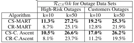
net-Table 4: Both our contributions are beneficial since a method that only fixes Issue 1 via the Cost-Reweighted adaption is outperformed by the Cost-Sensitive algorithms that fix both issues. Note that AdaRank cannot be Cost-Reweighted be-cause it is not a gradient ascent method.
RCS@kfor Outage Data Sets High-Risk Outages Customers Outages
Algorithm k=10 k=50 k=10 k=50
CS-MART 11.3% 27.2% 19.2% 25.3%
CR-MART 8.7% 25.1% 12.8% 21.9%
CS-C. Ascent 10.5% 26.6% 17.0% 26.2%
CR-C.Ascent 8.1% 23.7% 11.2% 19.5%
work areas are exposed to the same storm and therefore very similar wind/rainfall conditions. Regression’s ignorance of the ranking goal can thus lead to poor performance.
We also test whether our two fixes in Section 2 and 3 both contribute to performance: in Table 4, our Cost-Sensitive al-gorithms outperform the Cost-Reweighted version that ad-dresses only Issue 1 (the cost or importance of each list) but does not address Issue 2 (individual list cost-sensitivity) as intended. Similar results apply to the other data sets.
We will stress that the effectiveness of our Cost-Sensitive approach is measured by comparing the new CS or CR al-gorithm with its original counterpart in each pair; the large variance across different pairs is caused by the relevant ben-efits of each search strategy.
6. Acknowledgments
7. Conclusion
Experiments validate our Cost-Sensitive Learning to Rank paradigm. Our suite of Cost-Sensitive and Cost-Reweighted solutions outperform existing ranking methods which ignore a company’s use case: ranking to guide the prevention of costly damage. This solution is thus useful in diverse risk management domains, such as power outage prevention.
References
Bergeron, C.; Zaretzki, J.; Breneman, C.; and Bennett, K. P. 2008. Multiple instance ranking. InProceedings of the 25th International Conference on Machine Learning, ICML ’08, 48–55. New York, NY, USA: ACM.
Bian, J.; Liu, T.-Y.; Qin, T.; and Zha, H. 2010. Ranking with query-dependent loss for web search. 141–150.
Bukaty, R. F. 2013. Thousands in Maine remain without power, nearly a week after massive ice storm - The Boston Globe.
Burges, C. J. 2010. From ranknet to lambdarank to lamb-damart: An overview.
Cao, Z.; Qin, T.; Liu, T.-Y.; Tsai, M.-F.; and Li, H. 2007. Learning to rank: from pairwise approach to listwise ap-proach. InProceedings of the 24th international conference on Machine learning, 129–136. ACM.
Friedman, J. H. 2001. Greedy function approximation: a gradient boosting machine. Annals of statistics1189–1232. Guikema, S. D.; Nateghi, R.; Quiring, S. M.; Staid, A.; Reilly, A. C.; and Gao, M.-L. 2014. Predicting hurricane power outages to support storm response planning. Access, IEEE2:1364–1373.
2017. Insured losses for Europe’s storm Zeus estimated at US$200m: Perils.
Kankanala, P.; Das, S.; and Pahwa, A. 2014. Adaboost: An ensemble learning approach for estimating weather-related outages in distribution systems.Power Systems, IEEE Trans-actions on29(1):359–367.
Lawrence Berkeley National Laboratory 2004. Understand-ing the cost of power interruptions to U.S. electricity con-sumers.
Liu, T.-Y., et al. 2009. Learning to rank for information re-trieval. Foundations and TrendsR in Information Retrieval 3(3).
Maimon, O., and Rokach, L. 2005. Data mining for imbal-anced datasets: An overview. InData Mining and Knowl-edge Discovery Handbook.
Nateghi, R.; Guikema, S. D.; and Quiring, S. M. 2014. Fore-casting hurricane-induced power outage durations. Natural Hazards74(3):1795–1811.
CBC News 2015. B.C. storm: 22,000 customers remain without power - British Columbia - CBC News.
Niu, S.; Guo, J.; Lan, Y.; and Cheng, X. 2012. Top-k learn-ing to rank: labellearn-ing, ranklearn-ing and evaluation. In Proceed-ings of the 35th international ACM SIGIR conference on Re-search and development in information retrieval, 751–760. ACM.
Qin, T.; Liu, T.-Y.; Xu, J.; and Li, H. 2010. LETOR: A benchmark collection for research on learning to rank for information retrieval.Information Retrieval13(4):346–374. Sullivan, M. J.; Mercurio, M. G.; Schellenberg, J. A.; and Eto, J. H. 2010. How to estimate the value of service relia-bility improvements. 1–5.
Wang, J.; Song, Y.; Leung, T.; Rosenberg, C.; Wang, J.; Philbin, J.; Chen, B.; and Wu, Y. 2014. Learning fine-grained image similarity with deep ranking. In Proceed-ings of the IEEE Conference on Computer Vision and Pat-tern Recognition, 1386–1393.
Wang, X.; Bendersky, M.; Metzler, D.; and Najork, M. 2016. Learning to rank with selection bias in personal search. In Proceedings of the 39th International ACM SIGIR con-ference on Research and Development in Information Re-trieval, 115–124. ACM.
Wanik, D.; Anagnostou, E.; Hartman, B.; Frediani, M.; and Astitha, M. 2015. Storm outage modeling for an electric distribution network in northeastern usa. Natural Hazards
79(2):1359–1384.
Wu, Q.; Burges, C. J.; Svore, K. M.; and Gao, J. 2010. Adapting boosting for information retrieval measures. In-formation Retrieval13(3):254–270.
Xu, J.; Cao, Y.; Li, H.; and Huang, Y. 2006. Cost-sensitive learning of svm for ranking. In European conference on machine learning, 833–840. Springer.