Learning from Comparisons and Choices
Sahand Negahban [email protected]
Statistics Department Yale University
Sewoong Oh [email protected]
Department of Industrial and Enterprise Systems Engineering University of Illinois at Urbana-Champaign
Kiran K. Thekumparampil [email protected]
Department of Electrical and Computer Engineering University of Illinois at Urbana-Champaign
Jiaming Xu [email protected]
Krannert School of Management Purdue University
Editor:Qiang Liu
Abstract
When tracking user-specific online activities, each user’s preference is revealed in the form of choices and comparisons. For example, a user’s purchase history is a record of her choices, i.e. which item was chosen among a subset of offerings. A user’s preferences can be observed either explicitly as in movie ratings or implicitly as in viewing times of news articles. Given such individualized ordinal data in the form of comparisons and choices, we address the problem of collaboratively learning representations of the users and the items. The learned features can be used to predict a user’s preference of an unseen item to be used in recommendation systems. This also allows one to compute similarities among users and items to be used for categorization and search. Motivated by the empirical successes of the MultiNomial Logit (MNL) model in marketing and transportation, and also more recent successes in word embedding and crowdsourced image embedding, we pose this problem as learning the MNL model parameters that best explain the data. We propose a convex relaxation for learning the MNL model, and show that it is minimax optimal up to a logarithmic factor by comparing its performance to a fundamental lower bound. This characterizes the minimax sample complexity of the problem, and proves that the proposed estimator cannot be improved upon other than by a logarithmic factor. Further, the analysis identifies how the accuracy depends on the topology of sampling via the spectrum of the sampling graph. This provides a guideline for designing surveys when one can choose which items are to be compared. This is accompanied by numerical simulations on synthetic and real data sets, confirming our theoretical predictions. Keywords: Collaborative Ranking, Nuclear Norm Minimization, Multi-Nomial Logit Model
1. Introduction
Given data on how users compared subsets of items, we address the fundamental problem of learning a representation of users and items. Such data can be observed in the form
c
of choices (e.g. which item was bought) or in the form of comparisons (e.g. which items are rated higher). From such ordinal data on the items, we want to find low dimensional representations, which we call (latent) features, that explain crucial aspects of the users’ choices. Once learned, these features can be used to predict each user’s preference over items that the user has not seen yet, which can be used in recommendation systems and revenue management. These learned features also provide an embedding of the users and items on the same Euclidean space that allows us to directly quantify similarities via distances, that can be used to categorize and cluster. These embeddings can reveal the underlying structure of data such as images. Such an embedding of a discrete set of objects based on ordinal data has recently gained tremendous attraction mainly due to word embeddings based on co-occurrence data and their successes in numerous downstream natural language processing tasks Mikolov et al. (2013b).
The fundamental question in such a representation learning is: what makes one repre-sentation better than the others? Our guiding principle is that a good reprerepre-sentation is the one that defines a generative model that best explains the given data in the maximum likelihood sense. To this end, we focus on a parametric generative model known as Multi-Nomial Logit (MNL) model, widely used and studied in revenue management. The MNL model has a natural interpretation of human choices as an outcome of maximizing a utility by agents with noisy perception of the utility, also known asrandom utility modelin Walker and Ben-Akiva (2002); Azari Soufiani et al. (2012), defined as follows. Each user and item has a latent low-dimensional feature ui ∈Rr and vj ∈Rr respectively. The true utility of an item is the inner product of these two features Θij ,hhui, vjii=
P
kuikvjk. The inherent
low-rank structure of Θ = [Θij] captures the collaborative nature of the problem, where
users with similar preferences in the past are likely to prefer similar items in the future.
When presented with a set of items, a user reveals a noisy ordering of the items sorted according to her perceived utilities of the items, each of which is perturbed by an i.i.d. noise added to the true utility Θij. The MNL model is a special case where the noise follows the
such as embedding images using crowdsourcing Tamuz et al. (2011) and word embedding Mikolov et al. (2013b), whose connections we make precise in Section 6.
Motivated by recent advances in learning low-rank models, e.g. Negahban et al. (2009); Davenport et al. (2014), we ask the fundamental question of learning the MNL model from data on comparisons and choices. We provide a general framework using convex relaxations for learning the model. As data is collected in various forms on modern social computing systems, we consider the following four canonical scenarios:
• Pairwise comparisons. The most simple and canonical piece of ordinal data one can collect from a user at a time is a pairwise comparison; given two options, we ask the user which one is better. Such data is prevalent in the real world and is the most popular scenario studied in ranking literature, e.g. Shah et al. (2014). However, one significant aspect of the real data that has not been addressed in the literature is irregularities in the sampling. Consider an online seller with various products, say cars and watches. It does not make sense to ask a user to compare a car and a watch; one cannot sample an outcome of a comparison between a watch and a car. However, knowing a user’s preference on cars can help in learning her preference on watches. We want to propose a model and design an inference algorithm that can take into account such restrictions in sampling. We further want to quantify the gain in using all such data together in inference, as opposed to running inference in each category separately. To this end, we propose a new model for sampling that we call graph sampling. This model explains such irregularities in the real world data. We propose a novel inference algorithm tailored for the given sampling pattern. Our analysis captures precisely how the accuracy depends on the different topologies of the sampling.
• Higher order comparisons. Consider an online market that collects each of its user’s preference as a ranking over a subset of items that is ‘seen’ by the user. Such data can be obtained by directly asking to compare some items, or by indirectly tracking online activities on which items are viewed, how much time is spent on the page or how the user rated the items. However, collecting such comparisons over multiple items might come at a cost. We, therefore, want to quantify the gain in the accuracy of the inference when higher order comparison outcomes are collected. We characterize the optimal trade-off between accuracy and the number of items compared, and show that our proposed algorithm seamlessly generalizes to this setting and also achieves the optimal trade-off.
• Customer choices. One of the most widely applicable data collection scenarios is cus-tomer purchase history. Online and offline service providers can track each cuscus-tomer on which subset of items is offered and which item is chosen. Given historical data on such choices on best-out-of-a-subset, we extract features on the users and items that best explains the collected data.
together for one recipe or we buy two connecting flights. One choice (the first flight) has a significant impact on the other (the connecting flight). In order to optimize the assortment (which flight schedules to offer) for maximum expected revenue, it is crucial to accurately predict the willingness of the consumers to purchase bundled items, based on past history. We propose a model that can capture such interacting preferences for bundled items (e.g. jeans and shirts), and use this model to extract the features of the items in each category from historical bundled purchase data. Both our inference algorithm and the analyses extend to this setting, achieving the optimal trade-off between sample size and accuracy.
Contribution. We first study the canonical scenario of pairwise comparisons from the MNL model in Section 3. Our contribution in the modeling is a new sampling scenario we call graph sampling that captures how different pairs of items have varying likelihood of being compared together. Our algorithmic contribution is a convex relaxation with a new regularizer using a variation of the standard nuclear norm tailored for the graph sampling topology. Our theoretical contribution is in the analysis of the proposed estimator and a matching fundamental lower bound (up to a poly-logarithmic factor). This (a) characterizes the minimax sample complexity of the problem; (b) proves that the proposed estimator cannot be improved upon; and (c) identifies how the accuracy depends on the topology of sampling. This in turn provides a guideline for designing surveys when one has a choice on which pairs are to be compared. This is accompanied by experiments on synthetic and real data sets confirming our theoretical predictions.
This framework is extended to higher order comparisons in Section 4. We establish minimax optimality (up to a poly-logarithmic factor) of our estimator and identify the fundamental trade-off between accuracy and sample size. When each user provides a total linear ordering amongkitems, we show that the required sample size effectively is reduced by a factor of k. When the user provides her best choice (as in purchase history) instead of the total linear ordering, we extend our framework and establish minimax optimality in Section 5.2. We also consider a bundled purchase scenario in Section 5, where customers buy pairs of items from each of the two categories. We extend our framework and establish minimax optimality under the bundled purchase setting. We present experimental results on both synthetic and real-world data sets confirming our theoretical predictions and showing the improvement of the proposed approach in predicting users’ choices1.
Technically, we borrow analysis tools from 1-bit matrix completion Davenport et al. (2014), matrix completion Negahban and Wainwright (2012), and restricted strong con-vexity Negahban et al. (2009), and crucially utilize the Random Utility Model (RUM) Thurstone (1927); Marschak (1960); Luce (1959) interpretation (outlined in Section 2.1) of the MNL model to prove both the upper bound and the fundamental limit. This could be of interest to analyzing more general class of RUMs.
Notations. We use |||A|||F and |||A|||∞to denote the Frobenius norm and the `∞ norm, |||A|||nuc = P
iσi(A) to denote the nuclear norm where σi(A) denotes the i-th singular
value, and |||A|||2 = σ1(A) for the spectral norm. We use hhu, vii = P
iuivi and kuk to
denote the inner product and the Euclidean norm. All ones vector is denoted by 1, I denotes the identity matrix and I(A) is the indicator function of the event A. The set of the first N integers are denoted by [N] ={1, . . . , N}.
1.1 Related Work
Bradley-Terry and Plackett-Luce models. The simplest form of the MNL model is when all users are sharing the same feature vector such that each item is parametrized by a scalar value. This is known as Bradley-Terry (BT) model when pairwise comparisons are concerned and Plackett-Luce (PL) model when higher order comparisons are concerned. This has been proposed and rediscovered several times in the last century Zermelo (1929); Thurstone (1927); Bradley and Terry (1955); Luce (1959); Plackett (1975); McFadden (1973, 1980) in the context of ranking teams in sports games, ranking items based on surveys, and ranking routes in transportation systems. Unlike the general MNL model, maximum likelihood estimator for the BT and PL models are naturally convex programs. However, learning the BT model has first been addressed in Jr. (1957) where the convergence of the iterative algorithm is analyzed, without explicitly relying on the convexity of the problem. A new algorithm based on Majorize-Minimize framework was proposed in Hunter (2004). First sample complexity of learning BT model was provided in Negahban et al. (2012) where a novel estimator, called Rank Centrality, of the BT parameters was proposed. The authors construct a random walk over a graph where the nodes are the items and the transition probability is constructed from the comparisons outcomes. This spectral approach is proven to achieve a minimax optimal sample complexity. This has been a building block for several ranking algorithms, which further process the Rank Centrality to get better accuracy on top of it Chen and Suh (2015); Jang et al. (2016, 2017); Chen et al. (2017). For higher order comparisons, the sample complexity of learning PL model was provided in Hajek et al. (2014); Shah et al. (2014), where the Maximum Likelihood (ML) estimator is shown to achieve the minimax optimality. Later, Maystre and Grossglauser (2015) made the connection between the spectral approach of Rank Centrality and the ML estimator precise by providing a unifying random walk view to the problem. This led to a novel Accelerated Spectral Ranking algorithm introduced in Agarwal et al. (2018), which not only finds the parameters of the PL model more efficiently in computation, but also achieves optimal sample complexity under general sampling graphs. Recently, Borkar et al. (2016) treat the learning problem as solving a noisy linear system, and propose an algorithm that is amenable to on-line, distributed and asynchronous variants. Vojnovic and Yun (2016) analyzes a more general class of random utility models known as Thurstone models, and provide the minimax sample complexity by analyzing the ML estimator. Note that the ML estimators for Thurstone models in general are computationally intractable.
was proposed and analyzed under some separation conditions between the weights of the mixtures. For a mixture of two PL model, Chierichetti et al. (2018) shows identifiability and uniqueness of the mixture weights, when all marginal probability over all possible rankings among two items and three items are known. In a crowdsourced setting, Chen et al. (2013) models pairwise comparisons using a mixture of PL models consisting of hammer distribution, which reports the true output of a comparison, and spammer distribution, which reports the exact opposite of a comparison. A different approach that tackles the problem by learning to cluster the users based on the pairwise comparisons is proposed in Rui et al. (2015). The MNL model we study in this paper can be thought of as a generalization of the mixed PL models, where each user has her own preference. To make learning feasible, we inherently impose similarities among users via a low-rank condition. Note that a mixed PL model with r mixture is a special case of the MNL model with rank r, where each user’s membership is encoded as a r-dimensional feature in standard basis. In the context of collaborative ranking, algorithms for learning the MNL model from pairwise comparisons have been proposed in Park et al. (2015). Instead of nuclear norm regularization as we propose in this paper, Park et al. (2015) proposes solving a convex relaxation of maximizing the likelihood over matrices with bounded nuclear norm. Under the standard assumption of uniformly chosen pairs, it is shown that this approach achieves statistically optimal generalization error rate, instead of Frobenius norm error that we analyze.
Beyond BT and PL models. Modeling choice is an important problem where the ul-timate goal is to find the right parametric model to capture human choices. Ragain and Ugander (2016); Blanchet et al. (2013) use Markov chains to model choices with the param-eters in the transition matrix defining the probability model. Ideal point model Massimino and Davenport (2018); Kazemi et al. (2018) assumes that the pairwise comparisons of two items by a user depends on their distance from an ideal item (ideal point) for the user in some metric embedding space of the items. Novel nonparametric models have also been proposed to model human choices, for example Shah et al. (2016b); Pananjady et al. (2017); Fala-hatgar et al. (2018) uses strong stochastic transitivity to model pairwise choices and Farias et al. (2009) uses distribution over all permutations with sparse support to model higher order choices. We also note that in the context of (non-collaborative) ranking, Gleich and Lim (2011) has proposed nuclear norm minimization based algorithm when comparisons between all pairs items are modeled as a low-rank skew-symmetric matrix. Other non-parametric approaches to solving ranking include empirical risk minimization. Cl´emen¸con et al. (2005) analyses risk minimization of U-statistics and a more feasible surrogate con-vex loss minimization to estimate ranking. Katz-Samuels and Scott (2017) assumes that rating of an item by a user is a Lipschitz function of the user-item pair and analyses a nonparametric collaborative ranking algorithm from partial observation of such ratings.
2. Model and Approach for Pairwise Comparisons
The MultiNomial Logit (MNL) model is one of the most popular models that explains how people make choices when given multiple options and is widely used in behavioral psychology and revenue management. For brevity, we focus our discussion on data collected in the form of pairwise comparisons in Sections 2 and 3, and defer the discussion of the MNL model in its full generality to Sections 4 and 5 . We give a precise definition of the model for paired comparisons and provide a novel algorithmic solution to learn this model from samples.
2.1 MultiNomial Logit (MNL) Model for Pairwise Comparisons
Let Θ∗ be a d1×d2 dimensional matrix capturing preferences ofd1 users on d2 items. The probability with which a user, i⊆[d1], when presented with two items j1, j2⊆[d2], prefers itemj1 over itemj2 is,
P{j1 > j2}=
eΘ∗ij1
eΘ∗ij1 +eΘ∗ij2 . (1)
This implies that, more preferred items (as per the ordering of Θ∗ij) are more likely to be ranked higher, with the randomness in choices captured by the probabilistic model.
If we do not impose any further constraints on Θ∗, one entry of Θ∗ is not related in any way to any other entries. This implies that one user’s preference is completely independent of others’ and no efficient learning is possible. Each user’s preference has to be learned separately. On the other hand, in real applications, it is reasonable to say that preferences of users depend only on a handful of factors for example, quality, price, and aesthetics. We do not know which features affect users’ choices, but we assume that there arer-dimensional latent features for each of the users and items that govern such choices, and thatrd1, d2. This assumption mathematically captures the conventional belief that when two people have similar preferences over a subset of items, they tend to have similar tastes on other items as well. Formally, MNL model assumes that Θ∗ is a rank r matrix with r d1, d2. In this paper, we do not impose a hard constraint on the rank and provide general results for matrices of any rank. In this case, we identify how the accuracy depends on the rate of decay of the singular values.
This MNL model has many roots. In revenue management, this has been proposed as a special case of Random Utility Model (RUM). RUM explains choices that a person makes as the result of maximizing perceived random utilities associated with the set of alternatives presented. In the case of MNL, each decision maker and each alternative are associated with an r-dimensional vector, ui and vj, resulting in a low-rank Θ∗ if Θ∗ij =hhui, vjii. The
perceived utility of the itemj for decision makeriis,
Uij =hhui, vjii+ξij, (2)
whereξij’s are i.i.d. random variables following the standard Gumbel distribution. Different
2.2 Low-rank Regularization using Nuclear Norm Minimization
Given the low-rank structure of the model, a natural but inefficient approach is to minimize the negative of the log likelihood,L(·), regularized by the rank:
b
Θ ∈ arg min Θ∈Rd1×d2
−L(Θ) + λrank(Θ), (3)
for some parameterλ >0. As this rank minimization is a notoriously challenging problem, we instead solve a convex relaxation of it. Note that the nuclear norm ball is the convex hull of rank-1 matrices Recht et al. (2010). Analogous tol1-norm in the case of sparse vectors, nuclear norm is a tight convex surrogate for low-rank solutions. We propose the following nuclear norm regularized optimization problem,
b
Θ ∈ arg min
Θ∈Ω −L(Θ) +λ|||Θ|||nuc, (4) where Ω is a convex constraint which takes care of identifiability and Lipschitz smoothness conditions. Nuclear norm regularization has been widely used Recht et al. (2010) for rank minimization; however, provable guarantees exist only for quadratic loss functions L(Θ) Cand`es and Recht (2009); Negahban and Wainwright (2012). Our analyses extend such results to a convex loss, by first proving that −L(·) satisfies restricted strong convexity property with high probability. Similar to how (non-collaborative) rank aggregation has been generalized to any strongly log-concave distribution in Shah et al. (2014), our analysis can naturally be extended to a general class of strongly log-concave distributions. We give the expression for the log likelihood in Equation. (8) for pairwise comparisons.
3. Learning MNL Model from Pairwise Comparisons under Graph Sampling
Probabilistic model for sampling. In order to provide performance guarantees on the proposed approach, we need to specify how we sample the pairs that are to be compared. We provide a novel sampling model, which we callgraph samplingwith respect to a weighted graphG. This naturally generalizes Bernoulli sampling typically studied under matrix com-pletion literature Cand`es and Recht (2009); Keshavan et al. (2010a); Negahban and Wain-wright (2012); Jain et al. (2013), and the resulting analysis captures how the performance depends on the topology of the samples. Note that the proposed graph sampling is different from deterministic sampling graphs studied in Hajek et al. (2014); Shah et al. (2016a). This is analytically tractable only in the simpler case of estimating the weight vector of the PL model where there is only one user and the ML estimator is a convex program. However, such deterministic sampling is notoriously hard to handle for matrix estimation, even in the simpler case of matrix completion Bhojanapalli and Jain (2014). Hence, we introduce a probabilistic model that allows enough flexibility to capture the interesting aspects of sampling biases, i.e. grouping.
Precisely, we have a weighted undirected graph G = ([d2], E,{Pj1,j2}(j1,j2)∈E) with d2
nodes, which represent items, a set of edgesE and the edge weight Pj1,j2 between nodesj1
andj2. The weights can be written in a symmetric matrixP ∈Rd2×d2, andPj1,j2+Pj2,j1 =
that Pj,j = 0 ,∀j ∈ [d2], Pj1,j2 = Pj2,j1 and
P
j1,j2∈[d2]Pj1,j2 = 1. We assume we get
i.i.d. samples from first choosing a random user among [d1] users, and then choosing a pair (j1, j2) of items at random from P, and finally getting a random comparison from the MNL model, i.e. the probability with which user i prefers item j1 over item j2 is exp Θ∗ij1/
exp Θ∗ij1 + exp Θ∗ij2
.
One of the most important aspects of real-world data that is captured by this graph sampling model is grouping. Consider two groups of items, say, cars and phones. It does not make sense to ask an individual to compare a phone with a brand of a car (i.e. direct comparison is not feasible), but knowing an individual’s preference on cars can help in learning her preference on phones. In graph sampling terms, we are sampling from a graph G consisting of two disjoint cliques: one for cars and another for phones. By analyzing such a sampling scenario, we want to characterize the gain in using the data from both groups of items together, although there are no inter-group comparisons.
In the preference matrix Θ∗, the values in the set of columns corresponding to each connected component in the sampling graph can be arbitrarily shifted together, without changing the pairwise comparisons outcome distributions. This is because adding the same constant to those items that are compared does not change the probability (for those items within the same group), i.e.
P{j1 > j2} =
eΘ∗ij1 eΘ∗ij1 +eΘ
∗
ij2
= e
Θ∗ij
1+c eΘ∗ij1+c+eΘ
∗
ij2+c ,
and adding different constants to those items that are not in the same group does not change the probability of the outcome as those items are never compared. Hence, to handle this unidentifiability, we let a centered version of Θ∗ represent all those shifted versions defining the same probability distribution. Formally, let a zero-one vector gk ∈ {0,1}d2 denote the
group membership such that gi,k = 1 if item j is in group k, else gi,k = 0. Note that, by
definition, no item can be present in more than one group, that is,PG
k=1gk =1, where G
is the number of groups. We define an equivalence class of Θ∗ which represent the same probabilistic model as
[Θ∗] = nΘ∗+
G
X
k=1
ukgTk for all uk∈Rd1
o
. (5)
To overcome the identifiability issue, we represent each equivalence class with the centered matrix satisfying
Θ∗gk= 0, ∀k∈ {1,2, . . . , G} (6)
As matrices with large “spikiness” are known to be hard to estimate Negahban and Wainwright (2012), we capture the dependence of the sample complexity on the spikiness as measured byα :=|||Θ∗|||∞. This captures the dynamic range of the underlying preference matrix. For a related problem of matrix completion, where the lossL(θ) is quadratic, either a similar condition on`∞ norm is required or another condition on incoherence is required.
Graph Laplacian. The performance of our approach depends on the sampling graph P
via its graph Laplacian defined as
where diag(P1) is a diagonal matrix with P
vPu,v in the diagonals. Notice that, L is
singular and the nullspace is spanned by vectors{gk}G
k=1. Let σmax(L) =kLk2 andσmin(L) be the smallest eigenvalue of Ldiscounting theGzero-valued eigenvalues. Since the graph has G disconnected maximal components and L is real symmetric, by spectral theorem,
L = UΣUT, where U is a matrix of size d2 ×(d2−G) and its d2 −G columns form an orthonormal set, and Σ is a diagonal matrix such that its diagonal elements are the singular values of L. Let L† := UΣ−1UT and Lx := UΣxUT for all x ∈ R. We also define the Laplacian induced norms of matrices as,
|||Θ|||L:=
ΘL
1/2
F, and, |||Θ|||L-nuc:=
ΘL
1/2
nuc.
These Laplacian induced norms are more appropriate to analyze and quantify the distance between the estimated matrixΘ and Θb ∗.
When items k(i), l(i) are chosen for comparison by user j(i) as the i-th pair of items, we capture this choice with the matrix X(i) = ej(i)(ek(i) −el(i))T. The outcome of the comparison is represented by yi, withyi = 1 when item k(i) wins over iteml(i) and yi = 0 if otherwise. The log-likelihood of the comparison outcomes with respect to a parameter matrix Θ is,
L(Θ) = 1
n n
X
i=1
h
yihhΘ, X(i)ii −log
1 + exp
hhΘ, X(i)iii . (8)
We propose and analyze the following convex optimization problem,
b
Θ ∈ argmin Θ∈Ωα
− L(Θ) +λ|||Θ|||L-nuc, (9)
where,
Ωα =
n
Θ∈Rd1×d2 | |||Θ|||
∞≤α,Θgk = 0, ∀k∈[G]
o
, (10)
with an appropriately chosen λ= 8√2 max
q
σlog(2d)
n ,
σmin(L)−1/2log(2d) n
withσ = max{ (d2−G)/d1,1}, whered= (d1+d2)/2. In practice, the sampling probability distributionP and the corresponding Laplacian L might not be known. In those cases, we propose using the empirical sampling probability distribution ˆP and corresponding empirical Laplacian
ˆ
L instead. We describe this version of the algorithm formally in Section 3.4.4, where we empirically demonstrate the robustness of this approach. Further, in experiments with real data sets, we use the empirical Laplacian Section 3.4.5.
3.1 Performance Guarantee
We consider the graph sampling scenario where each sample is i.i.d., the`-th sample consists of user i` chosen uniformly at random, pair of items (j1,`, j2,`) chosen according to the
Theorem 1 Under the graph sampling with respect to G= ([d2], E, P) with a graph
Lapla-cian L, and under the MNL preference model with preference matrix Θ∗, solving the op-timization problem in (9) with n i.i.d. samples achieves, with probability greater than 1− 1/4d3,
1
d1
Θ∗−Θb
L1/2
F 2
≤36λ
α+ 1
ψ(2α) √
2r
Θ∗−Θb
L1/2
F+ min{d1,d2−G}
X
j=r+1
σj(Θ∗L1/2)
, (11)
for any r ∈ {1,2, . . . ,min{d1, d2 −G}}, any λ ≥ 8 √
2 max
q
σlog(2d)
n ,
σmin(L)−1/2log(2d) n
where σ = max{(d2 −G)/d1,1} and d = (d1 +d2)/2, ψ(x) , ex/(1 +ex)2, and for n ≤ min{26d21σ2,22 d1σmin(L)−1
2/3
}log(2d).
We provide a proof in Appendix A. The above bound holds for any r, where r allows us to trade off the two types of errors: the estimation error and the approximation error. Concretely, the above bound shows a natural splitting of the error into two terms; the first term corresponding to the estimation error for the top rank-r component of Θ∗ and the second term corresponding to the approximation error for how well one can approximate Θ∗ with a rank-r matrix. If we know the singular values of Θ∗, we can optimize over r
to get the tightest bound. If Θ∗ is exactly low-rank then applying a matching rank in the bound gives the following guarantee.
Corollary 2 (Exact rank-r matrix) Under the same hypothesis as in Theorem 1 with a
choice of λ= c0max
q
σlog(2d)
n ,
σmin(L)−1/2log(2d) n
for some c0 >0, if Θ∗ is exactly rank
r, there exists a positive constant c1 such that the proposed estimator achieves, 1
√
d1
Θ∗−Θb
L1/2
F ≤c1
α+ 1
ψ(2α)
√
rmax
r
σ d1log(2d)
n ,
p
(σmin(L)−1d1) log(2d)
n
, (12)
with probability at least 1−2/(d1+d2)3 andσ = max{(d2−G)/d1,1}.
The second term in the maximization is an artifact of the weakness of current analysis technique and does not reflect the actual error. This is confirmed in our simulation results on graphs with very small spectral gap in Figures 1.(b), (d), and (f), where the error in Laplacian-induced norm error does not decrease with spectral gap of L as the line graph has a much smaller spectral gap compared to a complete graph, for example. In fact, for a special Θ∗ in Figure 1.(d) it is the other way, for which we do not have a theoretical explanation.
The number of entries in Θ∗ is d1d2 and we want to rescale the Frobenius norm error appropriately by 1/√d1d2. As a typical scaling of L1/2 is 1/
√
only need to rescale the Laplacian-induced norm error by 1/√d1 in the left-hand side of the above bound. For a rank-r Θ∗, the number of degrees of freedom in describing it is
r(d1+d2)−r2 =O(r(d1+d2)). The above theorem shows that the total number of samples
nneeds to scale asO(r(d1+d2) logd) in order to achieve an arbitrarily small error. This is only a poly-logarithmic factor larger than the degrees of freedom. In Section 3.2 we make this comparison precise by providing a lower bound that matches the upper bound up to a logarithmic factor.
The upper-bound constraint in Theorem 1 on the number of samples n can be met for large enoughd1 and d2. For simplicity, assume that d1 =d2 =dandr is a constant. Since
σmin(L) =O(1/d2), the upper-bound on nbecomesO(max{d2, d4/3}). For large enoughd, the upper bound on the RHS of Eq. (12) can be made arbitrarily small withnonly scaling asO(r d). This is significantly smaller than the upper-bound ofO(d2) onn. Further, in the experiments in Section 3.4, we show that n has no practical upper-bound constraint since the error decreases at the same rate as predicted, for arbitrarily large values of n. This constraint may not be necessary and might be a by-product of the proof techniques.
The dependence on the dynamic range α, however, is sub-optimal. It is expected that the error increases with α, since the Θ∗ scales as α, but the exponential dependence in the bound seems to be a weakness of the analysis (for example as seen from numerical experiments in the right panel of Figure 6). Although the error increase withα, numerical experiments suggest that it only increases at most linearly. However, tightening the scaling with respect toαis a challenging problem, and such sub-optimal dependence is also present in existing literature for learning even simpler models, such as the Bradley-Terry model Negahban et al. (2012) or the Plackett-Luce model Hajek et al. (2014), which are special cases of the MNL model studied in this paper.
Another issue is that the underlying matrix might not be exactly low rank. It is more realistic to assume that it is approximately low rank. Following Negahban and Wainwright (2012) we formalize this notion with “`q-ball” of matrices defined as
Bq(ρq) ≡ {Θ∈Rd1×d2|
X
j∈[min{d1,d2}]
|σj(Θ∗)|q≤ρq}. (13)
When q = 0, this is a set of rank-ρ0 matrices. For q ∈(0,1], this is set of matrices whose singular values decay relatively fast. By optimizing the choice of r in Theorem 1, we get the following result.
Corollary 3 (Approximately low-rank matrices) Suppose Θ∗ ∈ Bq(ρq) for some q ∈
(0,1]and ρq>0. Under the hypotheses of Theorem 1, with a choice of λ=c0max
q
σlog(2d)
n ,
σmin(L)−1/2log(2d) n
for some constant c0 >0 there exists a constant c1 >0 such
that solving the optimization (9) achieves with probability at least1−2/(d1+d2)3, 1
√
d1
Θ∗−Θb
L1/2
F ≤ c1
√
ρq
√
d1
α+ 1
ψ(2α)
r
d2
1σ log(2d))
n
!2−2q
, (14)
This is a strict generalization of Corollary 2. For q = 0 and ρ0 =r, this recovers the exact low-rank estimation bound up to a factor of two. For approximate low-rank matrices in an `q-ball, we lose in the error exponent, which reduces from one to (2−q)/2.
3.2 Information-theoretic Lower Bound
For a polynomial-time algorithm of convex relaxation, we gave in the previous section a bound on the achievable error. We next compare this to the fundamental limit of this problem, by giving a lower bound on the achievable error by any algorithm (efficient or not). A simple parameter counting argument indicates that it requires the number of samples to scale as the number of degrees of freedom i.e., n ∝ r(d1 +d2), to estimate a
d1×d2 dimensional matrix of rank r. We construct an appropriate packing over the set of low-rank matrices with bounded entries in Ωα defined as (10), and show that no algorithm
can accurately estimate the true matrix with high probability using the generalized Fano’s inequality. This provides a constructive argument to lower bound the minimax error rate, which in turn establishes that the bounds in Theorem 1 is sharp up to a logarithmic factor, and proves no other algorithm can significantly improve over the nuclear norm minimization.
Theorem 4 SupposeΘ∗has a rankr. Under the previously described graph based sampling model, there exists a constant c >0 such that
inf b Θ
sup Θ∗∈Ω
α E
h 1
√
d1
Θ∗−Θb
L1/2
F
i
≥c min
e−α
r
r d1
n ,
αmax
s r
tr
L†r
,
d2 √
d1logd
)
, (15)
where the infimum is taken over all measurable functions over the observed comparison results and L†r is the pseudo inverse of the rankr approximation of the graph Laplacian.
A proof of this theorem is provided in Appendix B. The term of primary interest in this bound is the first one, which shows the scaling of the (rescaled) minimax rate as prd1/n and matches the upper bound in (12) up to a logarithmic factor. It is the dominant term in the bound whenever the number of samples is larger thann≥d1max{tr
L†r
, d1logd/d22}. As suggested in numerical simulations on graphs with very small spectral gap in Figures 1.(b), (d), and (f), the dependence in trL†r
is an artifact of the weakness of the current analysis technique. Here we note that, while the lower bound in Theorem 4 is in expec-tation, the upper bound in Theorem 1 is a high-probability result. The upper bound can immediately be translated into a bound in expected error with an additional term scaling asασmax(L)1/2
√
d2d−3, which is smaller than other terms in the bound. 3.3 Performance Guarantee and Lower Bound for Complete Graph
It follows from a simple relation |||(Θ∗−Θ)b L1/2|||F ≥σ
1/2
min|||Θ∗−Θb|||F, which is true since
Θ∗,Θ are in the range space ofb L, that the above upper bounds automatically give the error
with equal weightsPj1,j2 = 1/d2(d2−1), ∀j1 6=j2, Frobenius norm is the right metric and
we show matching upper and lower bounds.
Corollary 5 (Complete graph upper-bound) Under the same hypothesis as in
Corol-lary 2, if G is a complete graph, with a choice of λ = c0max
q
σlog(2d)
n ,
√
(d2−1) log(2d) n
for some c0 > 0, if Θ∗ is exactly rank r, there exists a positive constant c1 such that the
proposed estimator achieves,
Θ
∗−
b
Θ
F
p
d1(d2−1) ≤c1
α+ 1
ψ(2α)
√
rmax
(r
σ d1log(2d)
n ,
p
(d2−1)d1 log(2d)
n
)
, (16)
with probability at least 1−2/(d1+d2)3 andσ = max{(d2−1)/d1,1}.
Corollary 6 (Complete graph lower-bound) Suppose Θ∗ has rank r. Under the pre-viously described graph based sampling model with graph being a complete graph, there is a universal numerical constant c >0 such that
inf b Θ
sup Θ∗∈Ω
α E
h 1
p
d1(d2−1)
Θb−Θ
∗
F
i
≥cmin
e−α
r
r d1
n ,
αmax
(
1
p
(d2−1)
, √ d2
d1logd
) )
,
(17)
where the infimum is taken over all measurable functions over the observed comparison results.
3.4 Experiments
We provide a first-order method to solve the proposed convex optimization, and provide numerical experiments using this algorithm. We present two simulation results followed by an experiment on real data.
For the synthetic experiments, we generate random rank-r matrices of dimension d×
d, of the form Θ∗ = U VT with U ∈ Rd×r and V ∈
Rd×r entries generated i.i.d from uniform distribution over [0,1]. Then the connected-component-mean is subtracted form each connected component, and then the whole matrix is scaled such that the largest entry is α = 5. Note that this operation does not increase the rank of the matrix Θ. This is because this de-meaning can be written as Θ−P
kΘggT/(gT1) and both terms in the
operation are of the same column space as Θ which is of rankr.
3.4.1 Algorithm
Let Θ0 , ΘL1/2. As the nuclear norm regularizer in (9) is non differentiable, we use the proximal gradient descent Agarwal et al. (2010); Cai et al. (2010). At each iteration, we apply the following two operations on the current estimate, Θ0t, of Θ∗L1/2,
f
Θ0
t+1 = Θ0t−ηt∇ΘL(Θ0tL
whereMtΓtNtT :=fΘ0tis the singular value decomposition offΘ0t, such that Γt is a diagonal
matrix with positive entries, (·)+ is the entry-wise thresholding operation max(0, x), and ηt
is an appropriate step-size. Constraint of zero row sum, is taken care of by initializing the descent algorithm with Θ00 = 0, since rows of gradients sum to zero. In practice we do not know the value ofα, and hence in experiments we do not enforce thekΘk∞≤αconstraint.
Another issue in the implementation is that the convergence rate can be significantly slower for some graph topologies. We accelerate the proximal gradient descent with the following (modified) Barzilai-Borwein (BB) rule Barzilai and Borwein (1988) for choosing the step-size ηt,
ηt=
|||Θ0t−Θ0t−1|||22
hhΘ0
t−Θ0t−1,∇Θ0L0(Θt0)−∇Θ0L0(Θ0t−1)ii
, whent is odd hhΘ0t−Θ0t−1,∇Θ0L0(Θ0t)−∇Θ0L0(Θ0t−1)ii
|||∇Θ0L0(Θ0t)−∇Θ0L0(Θ0
t−1)|||22
, whent is even
, (20)
where ∇Θ0L0(Θ0) := ∇ΘL(Θ0L−1/2)L−1/2. We stop the descent algorithm whenever an upper bound of the KKT error is smaller than 10−5.
3.4.2 The Role of the Topology of the Sampling Pattern
In figure 1, we plot the error of our nuclear norm minimization based algorithm versus number of samples (in log-scale), nfor d1 =d2 = 300,r = 4, α= 5.0, G= 1. We consider two errors here; root mean squared error (RMSE) =
Θ−Θb
F/ √
d1d2 and Laplacian induced RMSE (L-RMSE)=
(Θ−Θ)b L
1/2 F/
√
d1. We plot these errors for four topologies of varying spectral gaps. As discussed Section 3.1, we do not expect the L-RMSE error to change much as we change the topology of sampling. However, as seen from the simple relation|||(Θ∗−Θ)b L1/2|||F ≥σ
1/2
min|||Θ ∗−
b
Θ|||F Frobenius norm error is more sensitive to the
topology of the sampling pattern, captured via the spectral gap, i.e. σmin(L). Specifically we use the following graph topologies.
• Complete graph. We first consider a uniform sampling over a complete graph where
Pj1,j2 = 1/d2(d2−1) for allj1, j2∈[d2]. The resulting spectral gap is 1/(d2−1), which
is the maximum possible value. Hence, complete graphs are optimal for learning MNL models, compared in the error metric of the Frobenius norm for fairness.
• Star graph. Here we choose one item to be the center, and every other items can only be compared to this center item uniformly at random. Let item 1 be the center one, then Pj1,1 = P1,j2 = 1/2(d2 −1). Standard spectral analysis shows that the
spectral gap is Θ(1/d2), and thus the graph is near-optimal for learning MNL models. • Line graph. Next, we consider a line graph withd2−1 edges wherePj,j+1 =Pj+1,j=
1/2(d2−1). It has a spectral gap of Θ(1/d22), and is strictly sub-optimal for learning MNL models.
(a) RMSE for i.i.d. Θ∗
ij (b) L-RMSE for i.i.d. Θ∗ij
(c) RMSE for barbell bias Θ∗ij (d) L-RMSE for barbell bias Θ∗ij
(e) RMSE for line bias Θ∗ij (f) L-RMSE for line bias Θ∗ij
Figure 1: Graphs with small spectral gap achieve significantly larger Frobenius norm error (RMSE)
Θ−Θb
F/ √
d1d2, whereas the Laplacian-induced norm error (L-RMSE)
(Θ−Θ)L1/2
uniformly at random for comparisons. The resulting spectral gap is Θ(1/d22), and this graph too is strictly sub-optimal for learning MNL models.
First in sub-figures 1a, 1b, we plot RMSE and L-RMSE errors for different graphs using randomly generated Θ∗ij. We see that L-RMSE curves for different graphs are the same (and slopes in log-scale are as expected approaches −1/2 with more samples). Further, we do not see any significant difference w.r.t the graph topology even when error is measured in Frobenius norm. The reason is that since Θ∗ij’s are generated i.i.d., the empirical distribu-tions of any large sub-group of items would be similar. Thus, the means of the two cliques of the barbell graph or the means of the items on the two far ends of the line graph are similar. Thus although barbell and line graphs have small spectral gap (high mixing-time), its effect is minimized because these sub-groups can individually be solved without having them to mix since the empirical distributions of the Θ∗ij in the two sub-groups are similar. To illustrate the role of the topology of the graph, we choose specific Θ∗ which depends on the topology of the graph as guided by our analysis on the lower bound (Theorem 4) in sub-figures 1c, 1d. The items are divided into two sets (corresponding to each side of barbell graph), such that corresponding Θ∗ij are i.i.d. inside a set but have similar but shifted means across the sets. We call this type of preference data as barbell biased. As expected from theoretical analyses, L-RMSE behave similar to the i.i.d. case. However, we see the Frobenius norm error significantly worse in the case of line and barbell shaped graphs, as expected from the Frobenius error bound. In sub-figures 1e, 1f, we simulateline biased preference data Θ∗. Items are ordered (in the order of the line graph), such that Θ∗ij’s have similar distributions but their means get shifted in an arithmetic progression as you go down the ordering. Again, Frobenius norm error is significantly larger for line and barbell graphs as spectral gaps are small.
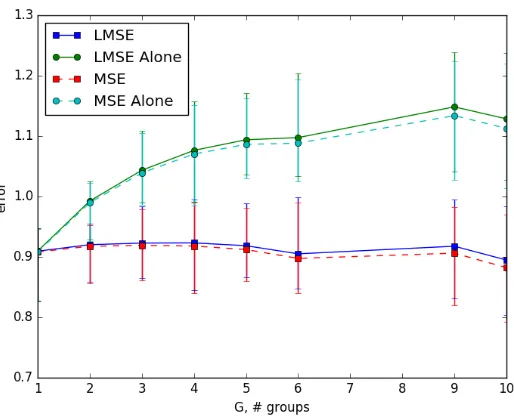
3.4.3 The Gain in Inference over Multiple Groups of Items
Consider Ggroups of items such that, within each group, every pair of items is uniformly likely to get compared, but items from different group are never compared with each each other. As a baseline, one can run inference on each group separately. On the other hand, we propose running inference on all the G groups jointly. Let Θ be the estimate of Θb ∗
when solving the groups together, and let ¯Θ be the estimate when groups are estimated separately. Let L, L(k) be the graph Laplacians of the whole graph and k-th connected component (group) respectively. suppose, for simplicity, that d1 = d2 and the groups are equally sized complete sub-graph components,
L= 1
(d2−G)
Id2×d2 − G d2
G
X
k=1
gkgkT
!
, and, (21)
L(k)= 1
(d2/G−1)
Id2 G×
d2 G
− G
d211
T
. (22)
According to Theorems 1 and 4, the L-RMSE error ofΘ satisfies,b
1 √
d1
Θ∗−Θb
L1/2
F =
1
p
d1(d2−G)
Θ
∗−
b
Θ
F = ˜O
r
rd1
n
!
Figure 2: As the number of groups increase, the gain in joint inference increases.
Similarly L-RMSE error (with respect to the full LaplacianL) of ¯Θ satisfies,
1
d1
Θ
∗−Θ¯
L1/2
F 2
= 1
d1(d2−G)
Θ∗−Θ¯
F 2
(24)
(a)
= (d2/G−1) (d2−G)
G
X
k=1
Θ∗k−Θ¯k
(L(k))1/2
2 F
d2
(25)
= 1
G G
X
k=1 ˜
O
rd1
n/G
(26)
= ˜O
Grd1
n
, (27)
where (a) follows from Eq. (22) and assuming Θ∗k,Θ¯k are sub-matrices restricted to the
columns in group k. Thus the estimation errors when running joint inference and sepa-rate inference for each group are of the order of OG(1) and OG(
√
G) respectively. That is, a user’s preference in one group of items will be useful in inferring the same user’s preference in another group of items. We illustrate this gain of joint inference in Figure 2. Concretely, the sampling graph G has G groups where each component is a complete graph and d1 = d2 = 360, r = 4, α = 5.0, n= 214. Figure 2 plots the L-RMSE (RMSE) =
(Θ−Θ)b L
1/2
F/ √
d1 (
(Θ−Θ)b
F/ √
103 104 105 106
number of comparisons, n 10-1
100
101
L-RMSE
line:
L
line:
L
ˆbarbell:
L
barbell:
L
ˆFigure 3: L-RMSE for various sampling graphs when true LaplacianLis known (solid) and when empirical Laplacian ˆL is used (dashed)
.
the groups separately the error increases with number of groups, although it is at a lower rate than predicted by the upper bound.
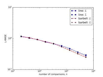
3.4.4 Robustness to the Mismatched L-nuc Norm Regularizer
In practical scenarios, one might not have access to the sampling graph Laplacian L. We propose using empirical Laplacian ˆL defined as
ˆ
L , diag ˆP1−P ,ˆ (28)
where ˆP ∈Rd2×d2 is the empirical distribution of sampled pairs in the given data. Under
the experimental setting from Figure 1b, we run additional experiments with this empirical Laplacian ˆL in the optimization: minimize −L(Θ) +λ|||Θ|||L-nucˆ . Figure 3 illustrates that the effect on the performance of not knowing the true L is marginal. Both approaches achieve the same error.
3.4.5 Real data: Food100
To showcase the practicality of our nuclear norm based algorithm (9) we apply our algorithm to the Food100 Data set2 Wilber et al. (2014). In the data set,n= 250320 triplets, denoted by{(ai, bi, ci)}i, of 3 distinct food dishes from a selection ofd= 100 were sampled. Then in
a crowdsourcing setting, users were asked if, ai is more similar tobi than toci. The goal is
to learn an low-dimensional embedding of the 100 food items where the above similarities are captured. We model the problem as learning an MNL model, parameterized by Θ∗, which gives the following probability distribution fori-th user’s answer,
P{ai is more similar tobi than toci} = e Θ∗ai,bi
eΘ∗ai,bi +eΘ∗ai,ci
.
This is the same model as the pairwise comparisons from Section 2, except for the fact that instead of a user (row) comparing two items (columns), here we compare a food item (row) to two other food items (columns). We implement three different algorithms: our nuclear norm based algorithm (‘nucnorm’), unregualrized (λ= 0) likelihood maximization (‘fullrank’) and maximum likelihood based algorithm to learn rank-1 Plackett-Luce model Luce (1959); Plackett (1975) (‘plackett’).
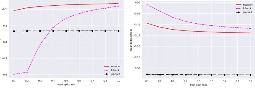
In Figure 4, we plot the mean log-likelihood of the learned model versus fractionxof the data used for training for the various algorithms for testing (a) and training (b) data. If x
fraction of the data is used for training, we use the rest (1−x) of the data for testing. For the nuclear norm minimization, we estimate the Laplacian L using the empirical distribution of the triplets andλis chosen to be 0.1plog(d)/2d xn.
In the Fig. 4(b) (to the left) on the testing data set, we see that our MNL model based nuclear norm regularized algorithm clearly outperforms both unregularized algorithm and the Placket-Luce model estimator, especially when there is less training data. In fact, the mean likelihood (log(Pmodel(test data))) on the testing data remains relatively the same when we decrease the size of the training data, which supports our claim that real data has low-rank structure. In the Fig. 4(b) (right) on the training data sets, the non-regularized approach of ‘fullrank’ achieves higher likelihood on the training data, indicating that it overfits to training data.
(a) Mean log-likelihood on testing data set (b) Mean likelihood on training data set
Dessert
Meat
Salad
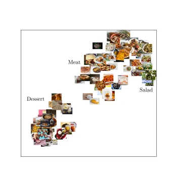
Figure 5: Food100: t-SNE embedding of the columns of the learned MNL parameter Θ.b
Desserts (bottom left) are seperated from other dishes. Meat dishes are also separated from vegetable dishes.
In Fig. 5 we plot the t-SNE embedding Maaten and Hinton (2008) of the columns of the estimated MNL parameter matrix Θ when all the data is used for training. The dessertsb
(left bottom) are separated from other dishes, and meat dishes and salad dishes form two clusters (top right).
4. Learning the MNL Model under Higher Order Comparisons
Si ⊆[d2], ofk alternatives she reveals her preferences as a ranked list over those items. To simplify the notations, we assume that all the users compare the same number kof items, but the analysis naturally generalizes to the case when the size might differ from a user to a user and when each user provides more than onek-wise ranking. Letvi,`∈Si denote the
(random) `-th best choice of useri. Each user gives a ranking, independent of other users’ rankings, from
P{vi,1, . . . , vi,k|Si is presented to useri}= k
Y
`=1
eΘ
∗
i,vi,`
P
j∈Si,`e
Θ∗i,j , (29) where with Si,` ≡ Si \ {vi,1, . . . , vi,`−1} and Si,1 ≡ Si. For a user i, the i-th row of Θ∗
represents the underlying preference vector of the user, and the more preferred items are more likely to be ranked higher.
Similar to the pairwise comparisons, the distribution (29) is independent of shifting each row of Θ∗by a constant. Since we can only estimate Θ∗up to this equivalent class, we search for the one whose rows sum to zero, i.e. P
j∈[d2]Θ ∗
i,j = 0 for alli∈[d1]. For capturing the
“spikiness” Negahban and Wainwright (2012) of Θ∗, we define α ≡ maxi,j1,j2|Θ ∗
ij1 −Θ
∗ ij2|
to denote the dynamic range of the underlying Θ∗, such that whenk items are compared, we always have
1
ke
−α ≤ 1
1 + (k−1)eα ≤ P{vi,1 =j} ≤
1
1 + (k−1)e−α ≤
1
ke
α , (30)
for all j ∈ Si, all Si ⊆ [d2] satisfying |Si| = k and all i ∈ [d1]. We do not make any assumptions onαother than thatα=O(1) with respect tod1andd2. Given this definition, we solve the following optimization
b
Θ ∈ arg min Θ∈Ωα
−L(Θ) + λ|||Θ|||nuc, (31) where,
L(Θ) = 1
k d1
d1
X
i=1
k
X
`=1
hhΘ, eieTv
i,`ii −log
X
j∈Si,`
exp hhΘ, eieTjii
, (32)
over
Ωα =
n
A∈Rd1×d2
|||A|||∞≤α, and ∀i∈[d1] we have X
j∈[d2]
Aij = 0
o
. (33)
Note that unlike graph sampling for pairwise comparisons, we assume that each user is presented a subset of k items and provides a complete ranking over those k items. This choice of sampling scenario, together with independent choices of the items in subsetSi’s, is crucial for getting a bound that is tight in its scaling with respect to not onlyd1,d2, and
r, but also k, as a certain independence is required to apply the symmetrization technique (in Lemma 29) which gives us the desired tight bound on the error. It trivially follows from our analysis that one can relax the assumptions in the sampling scenario significantly (e.g. sampling without replacement, heterogeneous sampling probabilities for each item-user pair, etc.), and the only change in the upper bound of Eq. (34) will be a weaker dependence
4.1 Performance Guarantee
We provide an upper bound on the resulting error of our convex relaxation, when amulti-set
of items Si presented to useri is drawn uniformly at random with replacement. Precisely, for a givenk,Si ={ji,1, . . . , ji,k}whereji,`’s are independently drawn uniformly at random
over the d2 items. Further, if an item is sampled more than once, i.e. if there exists
ji,`1 =ji,`2 for someiand `1 6=`2, then we assume that the user treats these two items as
if they are two distinct items with the same MNL weights Θ∗i,j
i,`1 = Θ ∗
i,ji,`2. The resulting
preference is therefore always overkitems (with possibly multiple copies of the same item), and distributed according to (29). For example, ifk= 3, it is possible to haveSi ={ji,1= 1, ji,2 = 1, ji,3 = 2}, in which case the resulting ranking can be (vi,1=ji,1, vi,2=ji,3, vi,3=
ji,2) with probability (eΘ∗i,1)/(2eΘ∗i,1 +eΘ∗i,2)×(eΘ∗i,2)/(eΘ∗i,1+eΘ∗i,2). Such a sampling with
replacement is necessary for the analysis, where we require independence in the choice of the items inSi in order to apply the symmetrization technique (e.g. Boucheron et al. (2013)) to
bound the expectation of the deviation (cf. Appendix C.4). Similar sampling assumptions have been made in existing analyses on learning low-rank models from noisy observations, e.g. Negahban and Wainwright (2012). Letd≡(d1+d2)/2, and let σj(Θ∗) denote thej-th
singular value of the matrix Θ∗. Define
λ0 ≡ e2α
s
d1logd+d2(logd)2(log 2d)4
k d21d2
. (34)
Theorem 7 Under the described sampling model, assume 24 ≤ k ≤ min{d21logd,(d21 +
d22)/(2d1) logd, (1/e)d2(4 logd2+ 2 logd1)}, and λ∈[480λ0, c0λ0] with any constant c0 =
O(1) larger than 480. Then, solving the optimization (31) achieves
1
d1d2
Θb−Θ
∗
2 F
≤ 288√2e4αc0λ0 √
r
Θb −Θ
∗
F+ 288e 4αc
0λ0
min{d1,d2}
X
j=r+1
σj(Θ∗), (35)
for anyr∈ {1, . . . ,min{d1, d2}}with probability at least1−2d−3−d−23whered= (d1+d2)/2. A proof is provided in Appendix C. This bound holds for all values of r and one could potentially optimize over r. We show such results in the following corollaries.
Corollary 8 (Exact low-rank matrices) Suppose Θ∗ has rank at most r. Under the hypotheses of Theorem 7, solving the optimization (31)with the choice of the regularization parameter λ∈[480λ0, c0λ0] achieves with probability at least1−2d−3−d−23,
1 √
d1d2
Θb −Θ
∗
F
≤ 288√2e6αc0
s
r(d1logd+d2(logd)2(log 2d)4)
k d1
. (36)
asO(rd1(logd) +rd2(logd)2(log 2d)4) in order to achieve an arbitrarily small error. This is only poly-logarithmic factor larger than the degrees of freedom. In Section 4.2, we provide a lower bound on the error directly, that matches the upper bound up to a logarithmic factor. The dependence on the dynamic rangeαis sub-optimal. The exponential dependence in the bound seems to be a weakness of the analysis, as seen from numerical experiments in the right panel of Figure 6. Although the error increase withα, numerical experiments suggests that it only increases at most linearly. A practical issue in achieving the above rate is the choice of λ, since the dynamic range α is not known in advance. Figure 6 illustrates that the error is not sensitive to the choice of λfor a wide range.
For approximately low-rank matrices in`q-ball defined in (13), optimizing the choice of r in Theorem 7, we get the following result. This is a strict generalization of Corollary 8 and a proof of this Corollary is provided in Appendix D.
Corollary 9 (Approximately low-rank matrices) Suppose Θ∗ ∈ Bq(ρq) for some q ∈
(0,1] and ρq > 0. Under the hypotheses of Theorem 7, solving the optimization (31) with
the choice of the regularization parameterλ∈[480λ0, c0λ0]achieves with probability at least 1−2d−3,
1 √
d1d2
Θb −Θ
∗
F ≤ 2√ρq
√
d1d2
288
√ 2c0e6α
s
d1d2(d1logd+d2(logd)2(log 2d)4)
k d1
2−q
2
.(37)
4.2 Information-theoretic Lower Bound for Low-rank Matrices
A simple parameter counting argument indicates that it requires the number of samples to scale as the degrees of freedom i.e., kd1 ∝ r(d1+d2), to estimate a d1 ×d2 dimensional matrix of rankr. By applying Fano’s inequality with appropriately chosen hypotheses, the following lower bound establishes that the bound in Theorem 7 is sharp up to a logarithmic factor.
Theorem 10 SupposeΘ∗ has rankr. Under the described sampling model, for large enough
d1 and d2≥d1, there is a universal numerical constant c >0 such that inf
b Θ
sup Θ∗∈Ω
α E
h 1
√
d1d2
Θb−Θ
∗
F
i
≥ cmin
(
αe−α
r
r d2
k d1
, √ αd2
d1d2logd
)
, (38)
where the infimum is taken over all measurable functions over the observed ranked lists
{(vi,1, . . . , vi,k)}i∈[d1].
A proof of this theorem is provided in Appendix E. The term of primary interest in this bound is the first one, which shows the scaling of the (rescaled) minimax rate as
p
r(d1+d2)/(kd1) (when d2 ≥d1), and matches the upper bound in (35). It is the dom-inant term in the bound whenever the number of samples is larger than the degrees of freedom by a logarithmic factor, i.e., kd1 > r(d1+d2) logd, ignoring the dependence on
4.3 Rank Breaking for Higher Order Comparisons
A common approach in practice to handle higher order comparisons isrank breaking, which refers to the practice of breaking the higher order comparisons into a set of pairwise com-parisons and applying an estimator tailored for pairwise comcom-parisons treating each pair as independent Azari Soufiani et al. (2013, 2014). When the higher order comparison is given as partial rankings (as opposed to total linear ordering as we assume) then rank breaking can be inconsistent, and special algorithms are needed for weighted rank breaking Khetan and Oh (2016a,b). However, when k-wise rankings (also called total linear orderings) are observed as we assume, simple and standard rank breaking achieves a similar performance as the higher order estimator in (31). Assume that ui,m, i ∈ [d1], m ∈ [k], denotes the
m-th element observed by the i-th user. Concretely, in rank breaking, we convert the k -wise ranking data into pair-wise ranking data and then we solve the following optimization problem:
L(Θ) = 1
d1 k2
X
i∈[d1]
X
(m1,m2)∈P0
Θi, hi(m1,m2)−log
expΘi, ui,m1
+ expΘi, ui,m2
,
(39)
whereP0={(i, j) : 1≤i < j ≤k}, andhi(m1, m2) andli(m1, m2) is defined as the higher and lower ranked index among ui,m1 and ui,m2 respectively. Then modified optimization
problem becomes,
b
Θ ∈ arg min Θ∈Ωα
−L(Θ) +λ|||Θ|||nuc (40) Letd≡(d1+d2)/2, and letσj(Θ∗) denote the j-th singular value of the matrix Θ∗. Define
λ0 ≡
s
dlogd k d21d2
. (41)
With this choice of regularization coefficient, we get the following upper bounds on the rank breaking estimator (40) that are comparable to the upper bounds of k-wise ranking estimator in Theorem 7 and Corollary 8.
Theorem 11 Under the described sampling model, assume2(c+ 4) logd ≤k≤ max{d1, d22/d1}logd, d1 ≥ 4, and λ ∈ [2
p
32(c+ 4)λ0, cpλ0] with any constant c = O(1)
larger than 2p32(c+ 4). Then, solving the optimization (40) achieves
1
d1d2
Θb −Θ
∗
2
F ≤ 144 √
2e2αcλ√r
Θb −Θ
∗
F+ 144e 2αcλ
min{d1,d2}
X
j=r+1
σj(Θ∗), (42)
for any r ∈ {1, . . . ,min{d1, d2}} with probability at least 1−2d−c−2d−2
13
where d = (d1+d2)/2.
Corollary 12 (Exact low-rank matrices) Suppose Θ∗ has rank at most r. Under the hypotheses of Theorem 11, there exists a constantc1 >0 such that solving the optimization (40) with the choice of the regularization parameter λ∈[2p32(c+ 4)λ0, cλ0]achieves with
probability at least 1−2d−c−2d−213, 1
√
d1d2
Θb−Θ
∗
F ≤ 144 √
2e2αc1
r
rdlogd k d1
. (43)
4.4 Experiments
We provide results from numerical experiments on both synthetic and real data sets.
4.4.1 Algorithm
Similar to the case of pairwise comparisons in Section 3.4.1, we use proximal gradient descent Agarwal et al. (2010); Cai et al. (2010) along with modified Barzilai-Borwein (BB) step-size selection rule Barzilai and Borwein (1988) with the initial point Θ0 = 0. Each iteration of the algorithm applies the following two operations on the current estimate, Θt, of Θ∗,
e
Θt+1= Θt−ηt∇ΘL(Θt) (gradient descent) (44)
Θt+1=Mt(Γt−ηtλI)+NtT (singular value shrinkage and thresholding) (45)
whereMtΓtNtT :=Θet is the singular value decomposition ofΘet, such that Γt is a diagonal
matrix with positive entries, (·)+ is the entry-wise thresholding operation max(0, x), and ηt
is an BB step-size calculated as,
ηt=
(
|||Θt−Θt−1|||22/hhΘt−Θt−1,∇ΘL(Θt)− ∇ΘL(Θt−1)ii, when t is odd hhΘt−Θt−1,∇ΘL(Θt)− ∇ΘL(Θt−1)ii/|||∇ΘL(Θt)− ∇ΘL(Θt−1)|||22, when t is even
.
(46)
4.4.2 Simulation: Higher Order Comparisons
The left panel of Figure 6 confirms the scaling of the error rate as predicted by Corollary 8. The lines merge to a single line when the sample size is rescaled appropriately (inset). We make a choice of λ=p(logd)/(kd2). This choice is independent of α and is smaller than proposed in Theorem 7. We generate the random rank-r true MNL parameters matrices of dimensiond×dusing the process mentioned in Section 3.4.1. The root mean squared error (RMSE) is plotted where RMSE = (1/√d1d2)|||Θ∗−Θb|||F. We implement and solve the
convex optimization (31) using proximal gradient descent method as analyzed in Agarwal et al. (2010). The right panel in Figure 6 illustrates that the actual error is insensitive to the choice of λfor a broad range of λ∈[p(logd)/(kd2),28p
(logd)/(kd2)], after which it increases with λ.
4.4.3 Simulation: Rank Breaking
100 1000 10000 100000 0.01
0.1 1
d=50, r=3 d=50, r=6 d=50, r=12 d=50, r=24
RMSE
sample sizek
0.1 1
1 10 100 1000 10000 100000
RMSE
λ √
(logd)/(kd2) α= 15
α= 10
α= 5
Figure 6: The (rescaled) RMSE scales aspr(logd)/kas expected from Corollary 8 for fixed
d= 50 (left). In the inset, the same data is plotted versus rescaled sample size k/(rlogd). The (rescaled) RMSE is stable for a broad range of λ and α for fixed d = 50 and r = 3 (right).
in Section 4.4.2, where we observe samples from k-wise ranking from an underlying true MNL model and the aim is to recover the true parameter Θ∗ of the model. We use
λ= 0.45p(logd)/(kd2) and λ= 0.1p
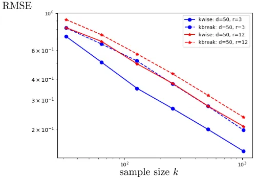
(logd)/(kd2) fork-wise and pairwise rank breaking algorithms respectively. In Fig. 7 we plot the RMSE for both the algorithm for d = 50 and r = 3,12. We note that the even though the RMSE decreases in the rate as predicted by the theorem, we see that pairwise rank breaking is worser than the higher orderk-wise algorithm which directly uses thek-wise rankings. This is consistent with the experimental observation made previously in Hajek et al. (2014). Further we note that rank breaking is much slower than the other algorithm, since gradient computation of the former takes
O(k2) time whereas for the latter it can be computed inO(k) time. 4.4.4 Real data: Jester
Jester data set3 Goldberg et al. (2001) has 24,982 users, each rating a subset of 100 jokes on continuous scale of [−10,10]. As the scale is continuous, we derive ordinal data from the scores (ties broken uniformly at random). We use only the 7200 users who rated all the jokes for our experiments. For each user, k = 100x jokes were randomly selected uniformly at random for training, rest of the 100−k = 100(1−x) jokes where used for testing, where x is the fraction of jokes selected for training. We implment four algo-rithms: nuclear norm minimization (‘nucnorm’) (31), unregularized (λ= 0) log-likelihood maximization (‘fullrank’), rank-1 Plackett-Luce model estimation (‘plackett’), and rank breaking algorithm (‘rankbreak’) (40). We use λ = 0.7p(0.5 log(d1d2))/(kd1
√
d1d2) and
λ = 0.16p(0.5 log(d1d2))/(kd1 √
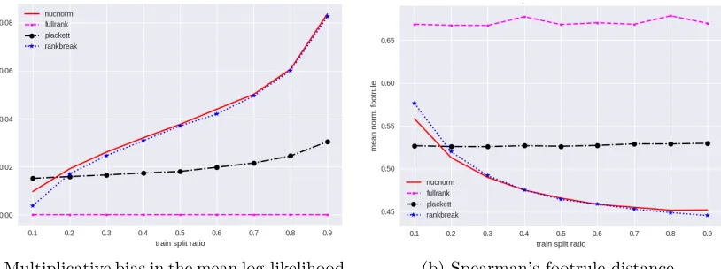
d1d2) for k-wise and pairwise rank breaking algorithms respectively. In Fig. 8 (a) we plot the multiplicative bias in the mean log-likelihood on the testing data versus the fraction x of training data used. For each model in {‘nucnorm’,
RMSE
sample sizek
Figure 7: Rank Breaking: RMSE error versus number of samples per userk. k-wise (‘kwise’) algorithm performs better than the rank breaking (‘kbreak’) approach.
‘fullrank’, ‘plackett’, ‘rankbreak’}, we plot in the y-axis
log(Pmodel(test data))−log(Pfullrank(test data)) |log(Pfullrank(test data))| ,
using fullrank model as a baseline as it has the least test likelihood. Plackett-Luce model achieves the best performance when sample size is small, as this simplest model avoids overfitting. However, for most regimes of sample size, both the nuclear norm minimization and rank breaking achieve similar performance improving upon the others.
The same trend holds when we measure the perfomrance in the normalized Spearman’s footule distance Diaconis and Graham (1977) F(π1, π2) ∈[0,1] between two rank-lists π1,
π2 of length k:
F(π1, π2) = 2
k2
k
X
i=1
|π1(i)−π2(i)|
In Fig. 8 (b) we plot the average normalized Spearman’s footrule distance between the ground truths and the most likely ranking on the testing data under the estimated model parameters. We see that k-wise nuclear norm minimization and rank breaking algorithms perform the best in recovering the true ranking, except when the fraction of training data used is very small so that the rank-1 Plackett-Luce recovers better ranking.
4.4.5 Real data: Irish Election
The Irish Election data set4 is an opinion poll conducted among 1083 participants during the 1997 Irish presidential election campaign Gormley and Murphy (2009). Each partici-pant responded with a ranking the of their top 1, 2, 3, 4, or 5 choices from the 5 candidates: