Advanced Control Methods for Cross-Flow Turbines
Benjamin Strom
1, Steven L. Brunton
2, and Brian Polagye
3,
Dept. of Mechanical Engineering, University of Washington
Stevens Way, Box 352600, Seattle, WA, 98195, USA
1
[email protected],
2[email protected],
3[email protected]
Abstract—Cross-flow turbines have a number of potential ad-vantages for hydrokinetic energy applications. Two novel control schemes for improving cross-flow turbine energy conversion are introduced and demonstrated through scale experiments. The first aims to alter the local flow conditions on the blades through varying blade kinematics as a function of rotational position, thus increasing beneficial fluid forcing. An established method accomplishes this by oscillating the mounting angle of the blade. Instead we proposed to vary the angular velocity of the blade as a function of azimuthal position. Optimizing this controller resulted in a 59% increase in turbine performance over standard controllers. The second control scheme operates an array of two turbines in a coordinated manner to take advantage of periodic wake structures. For a range of relative turbine positions, a parent controller maintains a constant blade position difference between turbines with the same angular velocity. For select positions, the array efficiency is shown to be greater than that of a single turbine. At the optimal position, coordinated control results in a 4% increase in array performance over uncoordinated operation. Finally, intracycle angular velocity and coordinated control schema are combined.
Index Terms—Hydrokinetic, Cross-Flow, Vertical-Axis, Tur-bine, Control
I. INTRODUCTION
Though axial-flow (horizontal-axis) turbines have become the standard turbine type for wind energy, cross-flow (vertical-axis) turbines have several key advantages for hydrokinetic energy applications. Cross-flow turbines, where the incoming flow direction is perpendicular to the axis of blade rotation, generally have a slower maximum blade speed than axial-flow turbines. This reduces the risks of blade-damaging cavitation, acoustic pollution, and harm to marine fauna. The bi- or omni-direction operation of cross-flow turbines may eliminate the need for active yaw control in reversing tidal flows. Cross-flow turbines have a rectangular cross-sectional area, making them more suitable for maximizing energy extraction from shallow tidal channels or rivers. Additionally, this geometry may allow for the construction of high blockage-ratio arrays, which can boost array performance [1]. Finally, there is evidence that arrays of cross-flow turbines may be able to outperform arrays of axial-flow turbines by beneficial device-device interactions, particularly when high array density is desired [2], [3].
Though in their simplest incarnation cross-flow turbines have just one degree of freedom, rotation about a central axis, their hydrodynamics are complex. This is because the local flow conditions experienced by the blades cyclically vary through one rotor rotation. Additionally, the wake generated by
the blade pass on the upstream side of the rotor is intercepted blades on the downstream side of the rotor. This complexity, however, presents unique opportunities for control not present in axial-flow systems. One such avenue is to vary the blade kinematics during the rotation to alter the varying local flow conditions, with the objective of increasing blade lift and decreasing drag, thus increasing turbine power output. Another opportunity stems from the fact that, under some operating conditions, coherent vorticies can be shed into the wake of cross-flow turbines. If downstream turbines are controlled in concert with upstream turbines, it may be possible to either avoid detrimental effects of these periodically shed coherent structures or take advantage of them, improving array performance. The objective of this study is to demonstrate and optimize specific implementations of both of these control opportunities through scale experiments.
Cross-flow turbine performance is characterized by the rotor mechanical efficiency, or the power coefficient, which is given by
CP =
τ ω
1 2ρU∞
3A (1)
whereτ is the torque produced by the turbine rotor,ω is the angular velocity, ρ is the fluid density, U∞ is the freestream velocity, and A is the cross-sectional area of the turbine rotor. This is the mechanical power produced by the turbine rotor, not including generator or bearing losses, normalized by the power available in the incoming flow. Cross-flow turbine performance is presented as a function of tip-speed ratio
λ= ωR U∞
, (2)
whereR is the turbine radius.
If flow induced by the turbine rotor is neglected, the local, or nominal angle of attack experienced by the blade can be written as a function of the blade azimuthal position, θ, as
αn(θ) =−Tan−1[sin(θ), λ+ cos(θ)] +αp, (3)
where Tan−1 is the four quadrant arctangent and αp is the
preset pitch angle. Here we define θ = 0 where the quarter-chord of the blade is traveling directly upstream. Similarly, the magnitude of the local flow velocity, normalized by the freestream velocity, here referred to as thenominalfreestream velocity, can be expressed as
Un(θ)∗=
|Un(θ)| U∞
=pλ2+ 2λcos(θ) + 1. (4)
SPECIAL ISSUE OF THE TWELFTH EUROPEAN WAVE AND TIDAL ENERGY CONFERENCE, 27 SEPTEMBER - 1 AUGUST 2017, CORK, IRELAND ©EWTEC 2017. THIS IS AN OPEN ACCESS ARTICLE DISTRIBUTED UNDER THE TERMS OF THE CREATIVE COMMONS ATTRIBUTION 4.0 LICENCE (CC BY
h p://creativecommons.org/licenses/by/4.0/). UNRESTRICTED USE (INCLUDING COMMERCIAL), DISTRIBUTION AND REPRODUCTION IS PERMITTED PROVIDED THAT CREDIT IS GIVEN TO THE ORIGINAL AUTHOR(S) OF THE WORK, INCLUDING A URI OR HYPERLINK TO THE WORK, THIS PUBLIC LICENSE AND A COPYRIGHT NOTICE.
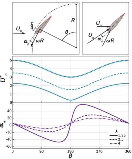
αp
c R
ωR
U∞ 4 θ
αn
U∞
Un
ωR
λ
U
* n
1 0 2 3 4 5
-40 -60 -20 0 20 40
0 90 180 270 360
1.25 2.5 4
α
nθ
Fig. 1. Top left, schematic definitions of the blade pitch angle, αp, as
measured at the quarter chord,c/4, the azimuthal blade position,θ, and the rotational velocity vector,ωr= dθdtr. The zero position,θ= 0, is defined for the foil traveling directly upstream. The top right defines the vector sum of the freestream velocity and the angular velocity as the nominal velocity, Un. Center plot: The nominal velocity profiles for a turbine operating at three
constant tip-speed ratios. Bottom: The nominal angle of attack profiles for the same three tip-speed ratios.
Vector diagrams describing nominal flow conditions and vari-ations with azimuthal blade position are shown in Fig. 1.
Depending on the tip-speed ratio, the nominal angle of attack can vary significantly over the rotation, far exceeding the static stall angle of the foil (see Fig. 1, bottom). A large dynamic pitching-up of a foil can result in a phenomenon known as dynamic stall. During this process, flow on the foil remains attached above the static stall point and a leading-edge vortex rolls up on the forward suction surface of the foil. This results in a lift force much greater than the maximum static-foil lift, as well as an increase in drag, often occurring slightly later than the increase in lift [4]. In cross-flow turbines, it may be beneficial to suppress dynamic stall to eliminate the large drag associated with separation [5]. However, birds [6], bats [7], and insects [8] have all been shown to take advantage the dynamic stall process. Dynamic stall has also been used to maximize the lift of a flapping flat plate [9], the thrust of an oscillating foil [10], and the power produced by a pitching and heaving foil [11]–[14]. Therefore, it may be possible to exploit dynamic stall to increase cross-flow turbine performance.
A. Intracycle Angular Velocity Control
Standard cross-flow turbine control consists of slowly (in comparison to on blade revolution) varying the angular ve-locity of the rotor in response to changes in the free-stream
velocity to maintain peak efficiency. A more advanced ap-proach consists of vary a control set-point as a function of the azimuthal blade position to optimize dynamic fluid forcing. We refer to this as intracycle control. One incarnation of intracycle control is to vary the blade mounting angle, αp,
as a function of blade position, similar to the rotor of a helicopter. This concept has been studied experimentally and numerically [15]–[17] and shown to result in efficiency gains of up to 24% [15]. A new, alternative control scheme, explored in detail in [18], is to vary the rotation rate, and thus the tip-speed ratio, as a function of blade position. As is evident by Eq. (3), this also results in changes to the nominal angle of attack profile, and thus the blade fluid forcing. Unlike preset-pitch control, the nominal freestream velocity profile is also altered. One distinct advantage intracycle variable velocity control has over pitch control is that it does not add mechanical complexity to the system.
In this study, two variable velocity profiles are studied, a sinusoidal
ω(θ) =A0+A1sin(N θ+φ1), (5)
and a semi-arbitrary (truncated Fourier series) profile
ω(θ) =A0+ 3 X
i=1
Aisin(iN θ+φi). (6)
Here, N = 2 is the number of blades, and ensures that each blade experiences the same kinematics. The wave-form parametersAiandφiwere optimized during experiments [18].
B. Coordinated Control
positioned at an optimal relative transverse position, identified by the previous experiment. At this position, a range of coordinated and uncoordinated control strategies are explored, including coordinated intracycle angular velocity control.
In summary, three series of experiments were performed. Optimization of intracycle angular velocity control profiles and comparison to standard control methods for a single turbine, a sweep of relative transverse position between two turbines with a comparison between coordinated and uncoordinated control, and optimization of coordinated intracycle angular velocity control for two turbines at a single relative position.
II. METHODS
A. Flumes
Turbine control schemes were explored experimentally in two recirculating flumes. The first is the Bamfield Marine Science Centre Flume and has a 2 meter wide, 10 meter long test section. The flume was operated at a dynamic depth of 0.73 m and a nominal velocity of 0.5 m/s. The freestream turbulence intensity was 3.5%. The second flume is the University of Washington Alice C. Tyler flume and has a test section measuring 0.75 m wide and 3 meters long. The dynamic depth was 0.47 m and experiments were performed at a freestream velocity of 0.7 m/s. Under these conditions, the turbulence intensity was 1.8%.
The blockage ratio, or the ratio of the turbine cross-section area to the flume test section cross section area was 11% and 2.6% for a single turbine in the Tyler and Bamfield flumes re-spectively. Because no generally accepted blockage correction exists for cross-flow turbines [23], efficiency magnitudes will not be compared between flumes. In the Tyler flume, efficiency values are likely higher than what would be measured in unconfined flow, but, we expect relative performance gains to be robust across blockage ratios.
B. Turbines
The turbines used in these experiments consisted of two straight NACA0018 foils atatched to circular endplates. The blades were mounted at a pitch angle of 6◦, leading-edge rotated outward about the quarter-chord. The turbine diameter was 17.2 cm and the height was 24.3 cm. For intracycle angular velocity control of a single turbine, a chord length of 4 cm was used. This was increased to 6 cm for both sets of coordinated control experiments in an attempt to increase the size of the coherent wake structures. The resulting solidities, calculated as the fraction of the circumference occupied by blades, were 15% and 22.5%. The turbines had 1.27 cm drive shafts. For the turbine used for the intracycle angular velocity control experiments and as the downstream turbine in the coordinated control studies, the upper end of this shaft was coupled to the servomotor, while the lower end was affixed to the bottom of the flume via a suction plate, load cell, and bearing. For the upstream turbine in coordinated control tests, the turbine was cantilevered on a 25 mm shaft mounted to the face of a servomotor.
Servo motors
Load cells
Load cell Turbine
Rotors
Bearing
U∞
Velocity or Torque Loop Current Loop
Motor Controllers
Computer
Real-Time Control
Data Acquisition
θ,ω ω
τ I
Fig. 2. Turbine test setups. The downstream setup is fixed and is used for single and dual turbine experiments. The upstream setup is used for dual turbine setups and is movable in the cross-stream wise direction via a robotic gantry. A computer with data acquisition cards and a real-time control kernel monitors and records encoder positions and turbine torques. Command signals are sent to motor controllers which operate the turbines under torque or velocity control.
C. Control and Data Acquisition
Turbines are controlled using servomotors (Yaskawa SGMCS-02B3C41) and motor controllers (Yaskawa SGDV-2R1F11). The servomotor control systems can absorb power from the turbines as generators as well as inject power into the turbines as motors. The motors can be operated in torque or velocity control mode. Internal encoders with106 counts per
revolution were used to measure the turbine azimuthal position and provided feedback for the angular velocity controllers. Six-axis load cells were used to measure turbine forces. The upper load cells (cantilevered: ATI Delta, non-cantilevered: ATI Mini45) were mounted between the servomotors and their mounting point, measuring the reaction torque between the servomotor and the turbine rotor. For the non-cantilevered tur-bine, the lower submersible load cell (ATI Nano25) measures the parasitic lower bearing torque applied to the turbine rotor. A schematic of the experimental setup is given in Fig. 2. The force, torque, and angular position measurements were acquired at a sample rate of 1 kHz over a period of 30 seconds for a given set of turbine control parameters. An acoustic Doppler velocimeter (Nortek Vector) was used to simultaneously measure the freestream velocity at a rate of 64 Hz at a location five diameters upstream of the most upstream turbine.
two turbines.
D. Efficiency Calculation
The turbine setups described above are designed to mea-sure turbine rotor mechanical efficiency. This metric excludes losses in bearings or the servomotors. In practice this mea-surement is made by assuming the control torque applied to the turbine rotor is thus sum of all forces internal to the servomotor, including electro-motive force and bearing losses. This is useful for optimizing efficiency of the fluid-rotor interaction, including fluid losses. Electrical and bearing losses due to the implementation of the proposed control schemes are the focus of a separate study [24].
Because a cross-flow turbine with two straight blades ex-periences significant variation in either angular velocity or torque output, efficiency values are always computed over an integer number of cycles. This to ensures mean efficiency is not skewed by instantaneously high or low power output. This becomes even more important for intracycle angular velocity control, where there are large torque fluctuations due to accelerating and decelerating the turbine. If considered separately from fluid forcing (including fluid losses), these acceleration torques integrate to zero over an even number of turbine rotations because the angular velocity profile is periodic.
To assess the success of control schemes applied to mul-tiple turbines, a metric of array efficiency is necessary. We propose a measure which normalizes the array power by the kinetic energy available accross the frontal area of the array. This metric would not be sensible if the turbine stream-wise spacing was large because energy from the surrounding flow would have significant time to reduce the wake deficit behind individual turbines. However, since the stream-wise spacing of these turbines is small (only 0.5D between the rotor edges) we feel it is appropriate to evaluate the array performance in this manner. In this way we can determine whether the array is performing better or worse than a single optimized turbine with the same frontal area (or two turbines spaced far enough apart to avoid flow interaction). The array performance for a pair of turbine is then defined as
CP, array=
ωupτup+ωdownτdown 1
2ρU∞3A∗
(7)
where
A∗= (
(D+|y|)H if |y|< D
2DH, if |y|> D (8)
whereD is the turbine diameter,H is the turbine height, and y is the distance between turbine centers in the transverse direction.
E. Experiment: Intracycle Angular Velocity Control
For this experiment, a single turbine with chord length of 4 cm is tested in the Alice C. Tyler flume at a freestream velocity of 0.7 m/s. The blockage ratio was 11.2% and the chord-based Reynolds number cU∞
ν
was 32,000. Two complete performance curves with the turbine operating under constant
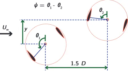
1.5 D
y
θ2
ψ = θ1 - θ2
θ1
U∞
Fig. 3. Diagram of the coordinated control experiment. The blade position difference between turbines, ψ, is defined as the position of a blade in the upstream turbine minus the position of a blade in the downstream turbine. Under coordinated control operationψis held constant.
torque and constant velocity control were taken. The peak CP of these curves were used for comparison with optimized
intracycle angular velocity control.
To optimize intracycle angular velocity control, values ofAi
and φi that maximized CP under intracycle angular velocity
control in Eqs. (5) and (6) were selected by the Nelder-Mead downhill simplex method [25] with the RS + S9 improve-ments for stochastic objective functions given in [26]. This optimizer was chosen due to the small number of required function evaluations. The optimization procedure consisted of first evaluating the mean turbine performance at a given set of Ai and φi, incrementing the parameters as indicated
by the Nelder-Mead algorithm, and finally implementing the upadated parameter set. Optimizations were performed five times with randomized starting conditions to ensure that the solutions converged to a global maximum.
F. Experiment: Coordinated Control
This experiment was performed with two turbines with chord lengths of 6 cm in the Bamfield Marine Science Center flume at a freestream velocity 0.5 m/s. The maximum blockage ratio (with the turbines side-by–side) was 5.5% and the chord-based Reynolds number was 34,000. The two turbines were spaced 1.5 diameters apart (center-to-center) in the stream-wise direction. The downstream turbine was fixed in place, while the upstream turbine was mounted to a gantry, allow-ing precise positionallow-ing in the transverse direction. Relative transverse positions of y/D = −2 → 2 were tested, with a resolution of 3 cm for |y/D| >1 and a resolution of 1 cm for |y/D| <1. The following results are presented as if the upstream turbine was fixed and the downstream turbine was moved because moving the downstream turbine through the wake of the upstream turbine is more intuitive. A diagram of this experiment is shown in Fig. 3.
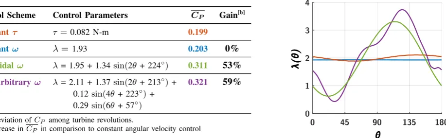
Control Scheme Control Parameters CP Gain[b]
Constantτ τ=0.082 N-m 0.199
Constantω λ=1.93 0.203 0%
Sinusoidalω λ= 1.95 + 1.34sin(2θ+ 224◦) 0.311 53%
Semi-arbitraryω λ= 2.11 + 1.37sin(2θ+ 213◦)+ 0.321 59%
0.12sin(4θ+ 223◦)+ 0.29sin(6θ+ 57◦)
[a]Standard deviation ofC
P among turbine revolutions. [b]Percent increase inC
P in comparison to constant angular velocity control 0 45 90 135 180 0
1 2 3 4
λ(θ)
θ
Fig. 4. Results from the intracycle angular velocity control optimization. Left: Optimum control parameters for the schemes tested, as well as their respective mean efficiencies (CP). The semi-arbitrary control scheme shows a 59% increase in efficiency over the constant angular velocity controller. Right: Tip-speed
ratio profiles of the optimum control schemes. A half revolution is presented as the profiles are twice periodic over a single turbine revolution. Note that the mean efficiency values presented are identical whether the total or fluid torque is used due to the angular velocity periodicity.
array. The first experiment explored “uncoordinated” control, where the downstream turbine was swept through a range of tip-speed ratios (λ = 0.5,0.7,0.9,1.3,1.5,and,1.7). In the second experiment both turbines were operated at the optimal tip-speed-ratio for an individual turbine (λ = 1.1), and the blade position difference (angular offset) between the blades of the two turbines was controlled and iterated from 0◦ to 171◦ in increments of 9◦.
G. Experiment: Coordinated Intracycle Angular Vel. Ctrl.
This experiment was performed in the Alice C. Tyler flume with the same pair of turbines as the prior coordinated con-trol experiment. The turbines were positioned in the optimal relative positions found from the co-rotating case of the coor-dinated control experiment (y/D=−0.81). Using the frontal area of the array, this resulted in a blockage ratio of 20.4%. The co-rotating case was chosen for this experiment because the co-rotating array performs identically if the freestream flow is reversed, making it more appropriate for tidal hydrokinetic energy applications.
A series of experiments were performed in this configu-ration. First, with both turbines operating under coordinated constant angular velocity control at the optimal tip-speed ratio for a single, isolated turbine, the blade position difference between turbines was swept from0◦to171◦in increments of 9◦. Second, under uncoordinated operation, the tip-speed ratios of both turbines were individually swept from λ= 1 →1.4 by increments of 0.1. This resulted in a4×4matrix of array performance. Finally, turbines were operated under sinusoidal intracycle angular velocity control in a coordinated manner, where the mean blade position difference between turbines was also controlled.
To ensure coordinated intracycle angular velocity control, the period of rotation for both turbines must be equal. For sinusoidal intracycle angular velocity control, assuming the servomotor perfectly recreates the commanded sinusoidal ve-locity profile, the turbine motion is described by the ordinary
differential equation
dθ
dt =A0+A1sin (2θ+φ). (9) The solution to this equation is
θ(t) =−1
2φ+ tan
−1
tan[t+C]pA2 0−A21
−A1
A0
(10) whereC is a constant that depends on the turbine position at t= 0. FindingC(t= 0) = 0and solving for the time required for one rotation yields a period of
T =p 2π A2
0−A21
. (11)
We now introduce the subscripts up anddown to differentiate
between upstream and downstream turbines. We also introduce the the ratio of the waveform amplitude to offset of the downstream turbine as
Rdown=
A1,down
A0,down
. (12)
Setting Tup =Tdown and and solving forA1,down and A0,down
yields
A0,down= s
A2 1,up−A
2 0,up
R2 down−1
(13)
and
A1,down=Rdown s
A2
1,up−A20,up
R2 down−1
. (14)
The motion of the two turbines is now completely parame-terized by A0,up, A1,up, φup, Rdown, φdown, and ψ, where ψ =
θup−θdown is the temporal mean blade position difference
between the two turbines. To enforce this mean position difference in an instantaneous manner, ψ(θup) is solved for
as a function of the position of the upstream turbine,θup. This
is done numerically by setting the constantCup in the equation
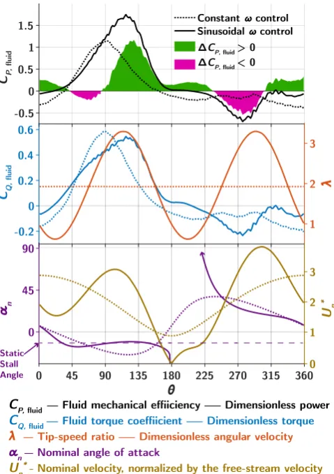
-0.5 0 0.5 1 1.5
CP, fluid
-0.2 0 0.2 0.4 0.6
CQ,
fluid
1 2 3
λ
0 45 90 135 180 225 270 315 360
θ
0 45 90
αn
0 1 2 3
Un
*
Constant ω control Sinusoidal ω control
ΔCP, fluid < 0 ΔCP, fluid > 0
Static Stall Angle
CP, fluid Fluid mechanical effiiciency Dimensionless power
CQ, fluid Fluid torque coeffiicient Dimensionless torque
λ Tip-speed ratio Dimensionless angular velocity
αn Nominal angle of attack
Un* Nominal velocity, normalized by the free-stream velocity
Fig. 5. Fluid power coefficient (top), fluid torque coefficient (center, blue), tip-speed ratio (center, red), nominal angle of attack (bottom, purple), and nominal freestream velocity (bottom, gold) for a one-bladed turbine under constant (dashed) and sinusoidal (solid) control are compared as functions of blade position. In the top plot,∆CP,fluidis difference in power coefficient between the sinusoidal and constant control schemes as a function of blade position. Green areas indicate greater power produced by the sinusoidal control scheme, while magenta indicates more power produced by the constant angular velocity control scheme.
equation forθdown(t)which results in a desired mean value of
ψ. The tandem turbine motion is then simulated and a vector values describingψ(θup)is generated. This vector is used for
realtime control of the turbine position difference such that the instantaneous blade position difference results in the desired mean value, given the angular velocity oscillations of both turbines.
The motion parameters are optimized using the same Nelder-Mead optimization scheme as in the intracycle angular velocity control experiment. In a final test, resulting optimized values of A0,up, A1,up, φup, Rdown, φdown are used, but ψ is
iterated from 0◦ to 171◦ by increments of 9◦. This test is to determine the importance of coordination for both turbines operating under intracycle angular velocity control.
III. RESULTS ANDDISCUSSION
A. Intracycle Angular Velocity Control
Fig. 4 shows the optimized angular velocity profiles and performance gains compared optimum constant torque control
and constant velocity control. These standard controllers per-formed similarly, at CP ≈ 0.20. We find increases in rotor
efficiency of 53% and 59% over constant velocity control for optimized sinusoidal and semi-arbitrary velocity waveforms respectively.
To examine the sources of success of intracycle angular velocity control, constant and sinusoidal velocity control was performed on a one-bladed version of the turbine. This allows for an approximate measurement of the forcing on a single blade of the two-bladed turbine. Examination of sinusoidal rather than semi-arbitrary angular velocity control was chosen because the smaller angular acceleration required make it more attractive for implementation.
The torque due to acceleration of the turbine rotor was removed from the power and torque measurements. This torque integrates to zero over a complete revolution, due to the periodic angular velocity profile. This allows for examination of the power coefficient due to the fluid forcing alone,
CP, fluid=
ω(τ−Jω˙) 1
2ρU 3
∞A
, (15)
where J is the mass moment of inertia of the turbine and servomotor rotor. Similarly the rotor torque coefficient due to fluid forcing alone is
CQ, fluid =
τ−Jω˙ 1
2ρU∞2AR
. (16)
Fig. 5 compares these values, along with the tip-speed ratio, nominal angle of attack, and nominal freestream velocity as functions of blade position. Under constant velocity control, fluid torque peaks at about θ = 90◦. During the power main power production region of the rotation, the nominal angle of attack under constant angular velocity control experiences a nearly constant ramp-up. Because the nominal angle of attack is well over the static stall angle (12◦ for NACA0018) at 21◦, it is likely that the foil is experiencing dynamic stall. Under sinusoidal control, the foil experiences a pitch-up and hold type maneuver to just over the static stall angle. This likely results in a slower leading-edge vortex formation, extending the increase in lift over a larger portion of the rotation. The result is an extended period of torque production, as evident from the CQ curve. An additional difference is
the nominal flow freestream velocity. Under constant angular velocity control, the nominal freestream velocity is decreasing during the power production portion of the cycle, while under sinusoidal angular velocity control, it is increasing rapidly. This may help the flow stay attached longer, or inject more energy into the leading-edge vortex. Additionally, a larger freestream velocity will increase the lift force.
Power is the product of the angular velocity and the rotor torque. Another source of success of the intracycle angular velocity controller is the alignment of the region of maximum torque production with maximum angular velocity, as evident by theCQandλcurves in Fig. 5. As a result, though the peak
-2 -1.5 -1 -0.5 0 0.5 1 1.5 2
Downstream Turbine Position, y/D
0 0.05 0.1 0.15 0.2
CP
CP (λopt)
CP, up ,λopt.
CP, down ,λopt.
CP, array λup = λopt
λdown = λbest
CP, array λup = λopt
λdown = λopt
Fig. 6. Summary of uncoordinated operation results from the coordinated control experiment. The optimal tip-speed ratio for a single, isolated turbine isλ = λopt.. The black dashed line, CP(λopt) indicates the performance of a single, isolated turbine at this tip-speed ratio. The blue and red lines, CP,upandCP,down, indicate the individual performance of the upstream and
downstream turbines respectively, with both turbines operating atλ=λopt.. Here, we have averaged performance over all blade position differences tested. We feel that this simulates uncoordinated control, as if the blade position difference was not dictated by a parent controller. The purple line is the array performance, Eq. (7), for these same conditions. The green, dashed line indicates peak array performance for the sweep of downstream turbine tip-speed ratios.
sinusoidal angular velocity control is 48% higher than under constant velocity control.
B. Coordinated Control
Fig. 6 summarizes the results of the effects of relative transverse turbine position on a two turbine array without coordinated control. Streamwise position was fixed at 1.5D. The black, dashed line indicates the peak performance of a single, isolated turbine. Power production is normalized by the power available in the freestream flow. It should be noted that due to induced flow, this is not necessarily representative of the power available to individual turbines in the array. Blue and red lines denote the individual performance of the upstream and downstream turbines respectively, where both turbines operate at the optimal tip-speed ratio of an isolated turbine. These values are calculated by taking the mean performance over blade position differences under coordinated control. This is equivalent to uncoordinated control performance, where the blade position difference is randomized. It should be noted that streamwise spacing is small enough that the upstream turbine performance (blue line) is negatively effected by the presence of the downstream turbine. Additionally, fast bypass flow around the upstream turbine boosts the downstream turbine performance (red line) over individual turbine efficiency for some positions on either side of the upstream turbine.
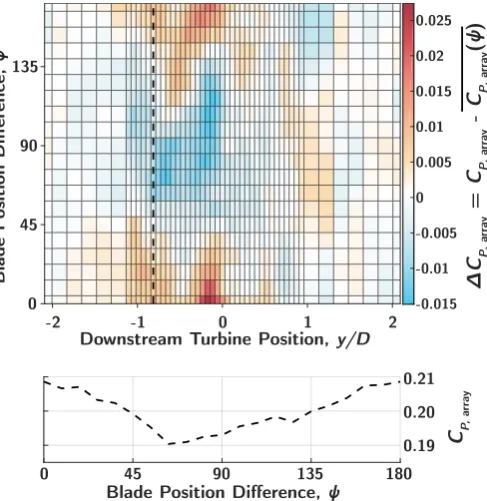
The purple line in Fig. 6 shows the array performance, according to Eq. (7), for the same case, where both turbines operate at the optimal tip-speed ratio for a single turbine. Again this is the averaged over blade-position differences under coordinated control. Of particular interest is that at
-2 -1 0 1 2
Downstream Turbine Position, y/D
0 45 90 135
Blade P
osition Difference,
ψ
Δ
CP, a
rra
y
=
CP, a
rra
y
-
CP, a
rra
y
(ψ
)
-0.015 -0.01 -0.005 0 0.005 0.01 0.015 0.02 0.025
0 45 90 135 180
Blade Position Difference, ψ
0.19 0.20 0.21
CP, ar
ray
Fig. 7. Top: Gain or loss in performance possible using coordinated control as a function of turbine relative position and blade position difference. Gain or loss is relative to mean performance across all blade position differences (the purple line in Fig. 6. The dashed line indicates the relative turbine position at which peak array performance occurs. Bottom: Array performance as a function of blade position difference at the relative turbine position of peak performance.
relative positions near y/D = −0.81, the densely packed turbine array outperforms a single turbine or a pair of dis-tantly separated turbines. This is due to the improvement in performance of the downstream turbine due to the accelerated bypass flow around the upstream turbine, and the fact that the frontal area of the array at this position is less than that of two turbines. The 6.7% increase in downstream turbine performance over isolated turbine performance agrees with the 7% increase found under similar conditions for wind energy-focused research via simulation in [19] and field measurements in [27].
In Fig. 6, the green, dashed line shows the best array performance resulting from the tip-speed ratio sweep of the downstream turbine. The upstream turbine is operated at the optimal tip-speed ratio for an isolated turbine. Array perfor-mance is increased by operating the downstream turbine at a lower tip-speed ratio when the turbines are aligned (near y/D = 0). Elsewhere, the greatest performance was found by operating both turbines at the optimal tip-speed ratio for a single turbine.
Control Scheme Control Parameters CP, array Gain[a]
Uncoord. Constantω λup=λdown=1.3 0.313 0%
Coord. Constantω λup=λdown=1.3 0.324 3.5%
ψ= 0◦
Uncoord. Sinusoidalω λup= 1.73 + 1.11sin(2θ + 199◦) 0.387 23.6%
λdown= 1.51 + 0.71sin(2θ + 226◦)
Coord. Sinusoidalω λup= 1.73 + 1.11sin(2θ + 199◦) 0.391 24.9%
λdown= 1.51 + 0.71sin(2θ + 226◦)
ψ= 80◦
[a]Percent increase inC
P, arrayin comparison to uncoordinated constant angular velocity control
0 45 90 135 180
θ
0.51 1.5 2 2.5 3
λ(θ)
Upstream Downstream
Fig. 8. A summary of results for the coordinated intracylce angular velocity control experiment. For uncoordinated constant angular velocity control, both turbines are operated atλ= 1.3. Via a sweep of tip-speed ratios of both turbine (see Fig. 9), this was found to result in peak array performance. Uncoordinated control efficiency was calculated as the mean performance over all coordinated control blade position differences. The peak array performance for coordinated constant angular velocity control is given in the second row. Optimized angular velocity profiles for coordinated control are shown to the right, corresponding to the third and fourth rows. Like the constant angular velocity results, the uncoordinated and coordinated sinusoidal angular velocity results are given as the mean and peak array performance for a sweep of mean blade position difference,ψ.
This leaves the variations in performance about the purple line in Fig. 6 which represents uncoordinated control at this tip-speed ratio. An increase in performance of∆CP, array= 0.027
and losses of ∆CP, array = −0.015 over the uncoordinated
case is shown to be possible. However, these large changes occur where the mean (overψ) array performance is poor, near y/D = 0. Fig. 7 (bottom) examines array performance as a function of blade position difference at the best position found for uncoordinated control,y/D =−0.81. This is position is indicated on Fig. 7 (top) as the vertical black dashed line. A modest, but significant 4% increase in efficiency is possible over uncoordinated array control at the optimal array position. With optimal relative turbine position and coordinated control, the array efficiency is CP, array = 0.209, which is a 12%
increase in efficiency over peak performance of an isolated turbine.
C. Coordinated Intracycle Angular Velocity Control
This experiment was performed with the turbines in the optimal position of y/D=−0.81found previously. Because of the differing Reynolds number and blockage ratio, the absolute magnitude of array performance cannot be compared to those of the previous sections. A summary of results is provided in Fig. 8.
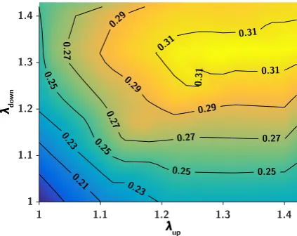
One of the limitations of the experiments of the previous section (realized after the fact) was that the tip-speed ratios of both turbines were not optimized for the uncoordinated control portion of the experiment; only the tip-speed ratio of the downstream turbine was altered. In Fig. 9, we show the results of a sweep of tip-speed ratios for both turbines under constant velocity, uncoordinated control. Peak array performance was found to be CP, array = 0.318 with both
turbines operating atλ= 1.3. Array performance was found to be insensitive to changes in upstream turbine tip-speed ratio betweenλ= 1.25→1.4. This may be because bypass flow around the the upstream turbine is increased with increased tip-speed ratio. This leads to more available energy for the
λup
λdown
Fig. 9. Results for a sweep of tip-speed ratios for two turbines operating under constant angular velocity uncoordinated control at the optimal relative position identified previously (y/D=−0.81). The upstream and downstream turbine turbine tip-speed ratios are on the X and Y axes respectively. Contour lines indicate array performance, Eq. (7).
downstream turbine, offsetting sub-optimal operation of the upstream turbine.
At this optimal tip-speed ratio (λ = 1.3), optimizing the blade position difference in coordinated control yielded a 1.9% increase in array performance, resulting in CP, array = 0.324.
The optimal blade position difference was ψ ≈ 0◦, which agrees well with the optimal blade difference found for this relative turbine position, as shown in Fig. 7 (bottom).
Fig. 8 (red lines) show optimized tip-speed ratio profiles for sinusoidal angular velocity control. These profiles were found while simultaneously optimizing the blade position difference φ. This adds a constraint to the angular velocity profile coefficients, as described in Eq. (12)→(14), ensuring that the period of one revolution is equal for both turbines.
mean blade position difference,ψ, was iterated from0→171◦ in increments of 9◦ while employing the optimized angular velocity waveform coefficients. The array performance was averaged over all blade position differences. This is termed uncoordinated sinusoidal angular velocity control, and is the array performance as if the the mean blade position difference was randomized. Uncoordinated sinusoidal angular velocity resulted in an array performance ofCP, array= 0.387, a 21.7%
gain over optimal uncoordinated constant angular velocity control. Coordinated sinusoidal angular velocity control at the optimal mean blade position difference resulted in an array performance of CP, array = 0.391, a 23% gain over
uncoordinated constant angular velocity control.
Two turbines under intracycle angular velocity control ap-pear to be less responsive to coordinated control than turbines under constant angular velocity control. The array efficiency increased only 1% when coordinated control was implemented on turbines under intracycle angular velocity control. This is in comparison to the 3.5% increase for constant angular velocity control, and the 4% increase observed in the previous experi-ment. This could be because intracycle angular velocity control is more robust in the face of disturbances to the freestream flow. Alternatively, efficiency increases for coordinated and intracycle angular velocity control could be additive rather than multiplicative. Another difference is the optimal blade position difference. For constant angular velocity control this is ψ = 0◦ while for variable angular velocity control it is ψ = 80◦. This difference may have to do with the structure and timing of vorticies shed by the upstream turbine, now modified by the new blade kinematics.
The optimal phase angle of angular velocity oscillation for both turbines was similar to that found in the inctracycle control experiment, despite the differing blade chord lengths. This experiment foundφup = 199◦ andφdown = 226◦ while
the intracycle control experiment found φ = 225◦ for the sinusoidal profile.
IV. CONCLUSION
Two novel control schemes for cross-flow turbines, intra-cycle angular velocity control and coordinated control have been introduced and tested in laboratory scale experiments. The combination of these two control schema is also explored. Intracycle angular velocity control is shown to boost the mechanical conversion efficiency of a single turbine as much as 59% for a single turbine. The magnitude of performance gain has the potential to change the landscape of the marine hydrokinetic industry and may result in cross-flow turbines becoming the technology of choice in future deployments. The efficiency increase is attributed to improvements in the local flow conditions experienced by the blades as well as an alignment of maximum torque production with maximum angular velocity.
Combining coordinated control with optimal relative turbine positioning resulted in an array performance increase of 12% over the efficiency of a single turbine. This allows for dense rotor packing while improving conversion efficiency. This
may result in significant gains in the the amount of energy extractable per unit area of seafloor, which is particularly important given the localized nature of tidal and river current resources. Additionally arrays of densely packed turbines designed to increase the blockage ratio of a tidal channel may not decrease individual turbine performance due to wake interaction. Further gains are possible if coordinated control is coupled with intracycle angular velocity control. Here an increase in dense array performance of 24.9% over standard control methods is demonstrated. Increases above this are likely possible if more complex angular velocity waveforms are applied to the individual turbines in the array or turbine geometry is optimized to be “exploitable” by the intracycle control scheme.
Future and ongoing work includes includes developing strategies for employing intracycle angular velocity control on commercial-scale turbines. This includes applying the control method to larger turbines. Tests using rotor cross-section area of 1.0 m2are planned. Additionally, the challenge of supplying
large power fluxes necessary for acceleration and deceleration of the rotor is being addressed. This includes exploring the feasibility of electrically coupling multiple turbines [24] as well as employing a custom gearbox. The gearbox consists of two sets of non-circular gears driven by a single generator. This applies the sinusoidal motion to two rotors, eliminating both the large transient power fluxes and control requirements on the generator by transferring the rotational kinetic energy between the rotors mechanically.
To fully describe the mechanisms responsible for perfor-mance increases of intracycle angular velocity control and coordinated control, flow measurements within and between rotors is necessary. Planar stereo particle image velocimetry measurements are planned for this purpose.
REFERENCES
[1] S. Salter, “Are nearly all tidal stream turbine designs wrong?” in 4th International Conference on Ocean Energy, 2012.
[2] R. W. Whittlesey, S. C. Liska, and J. O. Dabiri, “Fish schooling as a basis for vertical-axis wind turbine farm design,”Bioinspiration and Biomimetics, vol. 5, p. 035005, 2010.
[3] M. Kinzel, Q. Mulligan, and J. O. Dabiri, “Energy exchange in an array of vertical-axis wind turbines,”Journal of Turbulence, vol. 13, no. 38, pp. 1–13, 2012.
[4] W. McCroskey, “The phenomenon of dynamic stall.” National Aero-nautics and Space Administration Moffett Field CA, AMES Research Center, Tech. Rep., 1981.
[5] A.-J. Buchner, M. Lohry, L. Martinelli, J. Soria, and A. Smits, “Dynamic stall in vertical axis wind turbines: Comparing experiments and com-putations,”Journal of Wind Engineering and Industrial Aerodynamics, vol. 146, pp. 163–171, 2015.
[6] D. R. Warrick, B. W. Tobalske, and D. R. Powers, “Aerodynamics of the hovering hummingbird,”Nature, vol. 435, no. 7045, pp. 1094–1097, 2005.
[7] F. Muijres, L. Johansson, R. Barfield, M. Wolf, G. Spedding, and A. Hedenstr¨om, “Leading-edge vortex improves lift in slow-flying bats,”
Science, vol. 319, no. 5867, pp. 1250–1253, 2008.
[8] M. H. Dickinson, F.-O. Lehmann, and S. P. Sane, “Wing rotation and the aerodynamic basis of insect flight,”Science, vol. 284, no. 5422, pp. 1954–1960, 1999.
[10] F. Hover, Ø. Haugsdal, and M. Triantafyllou, “Effect of angle of attack profiles in flapping foil propulsion,”Journal of Fluids and Structures, vol. 19, no. 1, pp. 37–47, 2004.
[11] T. Kinsey and G. Dumas, “Parametric study of an oscillating airfoil in a power-extraction regime,”AIAA journal, vol. 46, no. 6, pp. 1318–1330, 2008.
[12] M. Ashraf, J. Young, J. S. Lai, and M. Platzer, “Numerical analysis of an oscillating-wing wind and hydropower generator,”AIAA journal, vol. 49, no. 7, pp. 1374–1386, 2011.
[13] Q. Xiao, W. Liao, S. Yang, and Y. Peng, “How motion trajectory affects energy extraction performance of a biomimic energy generator with an oscillating foil?”Renewable Energy, vol. 37, no. 1, pp. 61–75, 2012. [14] D. Kim, B. Strom, S. Mandre, and K. Breuer, “Energy harvesting
performance and flow structure of an oscillating hydrofoil with finite span,”Journal of Fluids and Structures, vol. 70, pp. 314–326, 2017. [15] B. Kirke, “Tests on ducted and bare helical and straight blade darrieus
hydrokinetic turbines,” Renewable Energy, vol. 36, no. 11, pp. 3013– 3022, 2011.
[16] I. Paraschivoiu, O. Trifu, and F. Saeed, “H-Darrieus wind turbine with blade pitch control,”International Journal of Rotating Machinery, vol. 2009, 2009.
[17] A. Sch¨onborn and M. Chantzidakis, “Development of a hydraulic control mechanism for cyclic pitch marine current turbines,”Renewable Energy, vol. 32, no. 4, pp. 662–679, 2007.
[18] B. Strom, S. L. Brunton, and B. L. Polagye, “Intracycle angular velocity control of cross-flow turbines,”Nature Energy (accepted, forthcoming), 2017.
[19] D. B. Araya, A. E. Craig, M. Kinzel, and J. O. Dabiri, “Low-order modeling of wind farm aerodynamics using leaky rankine bodies,”
Journal of renewable and sustainable energy, vol. 6, no. 6, p. 063118, 2014.
[20] J. Bremseth and K. Duraisamy, “Computational analysis of vertical axis wind turbine arrays,”Theoretical and Computational Fluid Dynamics, vol. 30, no. 5, pp. 387–401, 2016.
[21] K. Duraisamy and V. Lakshminarayan, “Flow physics and performance of vertical axis wind turbine arrays,” in32nd AIAA Applied Aerodynam-ics Conference, 2014, p. 3139.
[22] M. Ahmadi-Baloutaki, R. Carriveau, and D. S. Ting, “A wind tunnel study on the aerodynamic interaction of vertical axis wind turbines in array configurations,”Renewable Energy, vol. 96, pp. 904–913, 2016. [23] H. Ross and B. L. Polagye, “Blockage effects on current turbine
performance and wake characteristics,” in European Wave and Tidal Energy Conference, 2017.
[24] R. J. Cavagnaro, B. Strom, B. Polagye, and A. Stewart, “Power collec-tion from multiple hydrokinetic generators utilizing advanced control,” inEuropean Wave and Tidal Energy Conference, 2017.
[25] J. A. Nelder and R. Mead, “A simplex method for function minimiza-tion,”The computer journal, vol. 7, no. 4, pp. 308–313, 1965. [26] R. R. Barton and J. S. Ivey Jr, “Nelder-mead simplex modifications
for simulation optimization,”Management Science, vol. 42, no. 7, pp. 954–973, 1996.
[27] J. O. Dabiri, “Potential order-of-magnitude enhancement of wind farm power density via counter-rotating vertical-axis wind turbine arrays,”