Classifier-Based Evaluation of Image Feature Importance

Volume 55, 2018, Pages 162–175

GCAI-2018. 4th Global Con-ference on Artificial Intelligence

Classifier-Based Evaluation of Image Feature Importance

Sai P. Selvaraj

, Manuela Veloso

, and Stephanie Rosenthal

1

[email protected], Carnegie Mellon University, Pittsburgh, USA

2

[email protected], Carnegie Mellon University, Pittsburgh, USA

3

[email protected], Chatham University, Pittsburgh, USA

Abstract

Significant advances in the performance of deep neural networks, such as Convolutional Neural Networks (CNNs) for image classification, have created a drive for understanding how they work. Different techniques have been proposed to determine which features (e.g., image pixels) are most important for a CNN’s classification. However, the important fea-tures output by these techniques have typically been judged subjectively by a human to assess whether the important features capture the features relevant to the classification and not whether the features were actually important to classifier itself. We address the need for an objective measure to assess the quality of different feature importance measures. In particular, we propose measuring the ratio of a CNN’s accuracy on the whole image com-pared to an image containing only the important features. We also consider scaling this ratio by the relative size of the important region in order to measure the conciseness. We demonstrate that our measures correlate well with prior subjective comparisons of impor-tant features, but imporimpor-tantly do not require their human studies. We also demonstrate that the features on which multiple techniques agree are important have a higher impact on accuracy than those features that only one technique finds.

1

Introduction

There has been tremendous advancement in the performance of deep neural networks (DNNs), specifically in the task of image recognition using Convolutional Neural Networks (CNNs) [6]. As their popularity increases, there is much interest in understanding and explaining how these complex networks work. A variety of techniques have been proposed to indicate which pixel features are most discriminative for CNNs in determining their classification prediction on a given image (i.e., which pixels are most helpful in determining which class the image belongs to) [9,10,20]. For example, Simonyan et al. [10] use the gradients of the CNN’s classification probability with respect to the input pixels to determine which pixels are important. Zint-graf et al. [20] propose that the pixels which are most discriminative are the ones that, when occluded, most reduce the classification probability.

[9, 15,20] and use human studies to determine which regionspeople believe are most discrim-inative for their own classification. However, people’s opinions of important features may be different from what the CNN actually uses to determine its classification.

In contrast to subjective measures, one recent objective method was proposed to evaluate pixel importance by perturbing one random pixel at a time and then reclassifying the per-turbed images to observe how much the CNN prediction probability decreases [8]. The more the probability decreases, the higher the importance. However, the non-determinism in the perturbations could introduce new artifacts in the image which might affect classification in unknown ways. For example, if a perturbation in a pixel changes the CNN classification from dog to cat, it is unclear whether the change is because the classifier can no longer see the dog in the picture (i.e., its probability decreased) or because it suddenly starts seeing a cat as well (i.e., the probability of cat increases).

In this work, we also propose that feature importance should be measured objectively with respect to the predicting CNN. Like Samek et al. [8], our goal is to evaluate different techniques based on their capability to capture the features in the image that most affect the accuracy of the CNN. However, unlike the prior work that measured the decrease in accuracy caused by perturbing pixels in the image, we contribute metrics that begin with an uninformative baseline image and measure the increase in accuracy (confidence) caused by adding the important pixels. We call this metric Simple Confidence Gain (SCG).

SCG only considers the accuracy difference caused by adding features, but it does not consider several other measures of the important feature regions. First, we note that the maximal value of SCG occurs when all of the images pixels are labeled as important. A measure of the conciseness of the important features may help differentiate different importance algorithms. Similarly, the important features may increase the classifier accuracy but the CNN may still classify the important features incorrectly. Our second metric - Concise Confidence Gain (CCG) - builds upon SCG by also taking into account the conciseness of the region of pixels required to classify the image correctly. The smaller the region of important pixels that results in a correct classification, the higher the CCG score.

Using our metrics, we contribute objective comparisons of three different algorithms for finding important pixels on two different image datasets - Place365 [19] and our own dataset containing images of various floors in our building. The results from our metrics are internally consistent and correlate well with prior subjective comparisons of important features. However, we note that this may not always be a good check on the performance of the important features for the classification because people may not know what pixels are important to the classifier.

Additionally, we noticed that there is very little overlap in the important regions found by different algorithms. Given this finding, we contribute a technique to find more concise impor-tant pixel regions by identifying the pixels that are in agreement between different algorithms (i.e., the intersection regions). We demonstrate that these intersecting regions trade-off CNN accuracy with conciseness and represent an alternative approach to increasing the conciseness, compared to developing a new algorithm specifically to finding concise important features or reducing the size of another algorithm’s important features.

2

Related Work

A variety of deep network techniques have been developed to understand CNNs. We roughly divide these techniques into two categories - class model visualization and image specific vi-sualization. Class model algorithms such as Simonyan et al. [10], Yosinski et al. [14], aim to understand how the neurons in the network contribute to the classification. This is similar to the prior work identifying important features for classical machine learning algorithms in which the important features are the same for all data points [2, 3, 13]. In contrast, image specific techniques aim to find which features (pixels) the CNNs find most informative for the given image [7,9,10,15,16,20]. In this work, we focus on evaluating image specific techniques for the important features that they highlight. We refer to the feature-finding algorithms asimportance functions. For example, Simonyan et al. [10] have developed techniques to backpropagate the gradients of the CNN’s classification probability with respect to the input pixels to determine which pixels are important. The work has been extended to infer the important pixels from the activations of particular neurons in the CNN rather using gradients of the images directly [16]. Zeiler and Fergus [15] have developed a technique that occludes patches in the image and infer the important pixels in the image based on how much different patches decrease the CNN clas-sification accuracy. Zintgraf et al. [20] builds upon that procedure by using variable occluding patches – varying the size and the color. All of these importance functions have demonstrated an ability to determine the important pixels in an image.

With so many different algorithms, one major open question is which ones perform better than others and under what conditions. We are particularly interested in systematically com-paring these algorithms with respect to how well they identify the pixels that the CNN uses to classify them. There are relatively few evaluation techniques for analyzing or comparing importance functions. Both Selvaraju et al. [9] and Zhang et al. [16] evaluate their importance functions based on data collected from “pointing game” studies in which a person highlights the ground-truth pixels that contain the object to be detected. The importance functions are then evaluated based on where their outputted most important pixel lies relative– inside or outside, to the human annotated ground-truths. Better important functions have higher score in this pointing game evaluation. Similarly, Zeiler and Fergus [15] and Zintgraf et al. [20] depend on the reader’s inspection of different important regions to determine which importance function is better. Selvaraju et al. [9] use direct human studies in which a person is asked to determine which CNNs are more accurate based on how well each CNN’s important region reflects the classification object. This metric serves as an indirect measure of the importance function, as it assumes that better classifiers also find better important regions. To summarize, all of these evaluations use people to subjectively determine whether the important region contains object being classified.

Interestingly however, the evaluation techniques do not evaluate whether those pixels in the identified importance regions contributed most to the CNN’s classification and therefore may not necessarily result in a better understanding of the CNN’s actual functionality. For example, an image of a polar bear may not be classified as polar bear due to the bear itself (as a person may determine) but instead due to the wintry background around the bear. Additionally, it is challenging to extend the prior evaluation techniques to other classification tasks beyond object recognition which aims to localize an object in the image. For example, in the case of location recognition for robots, it would be challenging to ask a person what parts of an image identify it as the 3rd floor.

features. Samek et al. [8] proposes an algorithm that randomly perturbs a small region around the most important 100 pixels– proposed by the importance function being evaluated, of the image sequentially in the order of their importance and then uses the profile of the changes in classifier confidence scores to compare different importance functions. However, since the work randomly perturbs the pixels of the images, it could introduce new unintended artifacts– because of the non-determinism in the approach, in the image which might confuse the classifier. Also, the approach is time-consuming as it requires the classifier to be run 1000 times to evaluate an importance function with a single image.

We contribute new metrics for objectively evaluating importance functions that overcome the drawbacks to Samek et al. [8] discussed above. Our proposed metrics are 100 times faster than the prior approach and are deterministic. While we evaluate our new metrics on the three importance functions in this work, our metrics can be applied to any techniques that find features that are important to classifiers. We demonstrate the working of our metrics by ranking the importance functions on two scene recognition datasets, and we show that our ranking is consistent and correlates with prior subjective evaluations.

3

Importance Functions

We first formalize the definition of an importance function before proposing metrics for evaluat-ing them. We assume that a CNN classifierC outputsp(I=y|w), the probability of an image

I ∈ [0,1]c∗N with c channels (i.e., 3 for RGB) and N pixels having classification y given the trained weightsw. For clarity, we will refer to theith pixel in the image asI[i]. GivenC and

I, an importance function importance(I, C, y) outputs aheat map H ∈[0,1]N _{that contains a} measure of relevance or importance of each pixel I[i] to the class y. A variety of importance functions, each with their own heat map, have been proposed for explaining the classification predictions of CNNs. In this section, we briefly summarize the three algorithms that will be used for evaluating our metrics.

Occluding Patches (occ)[10]. The idea behind this approach is if a important feature in an image gets occluded, then the classifier’s prediction probabilityp(I=y|w) will fall. Specif-ically, a gray square patch of a fixed size, called the occlusion patch, is used to systematically occlude parts of the input image, and the prediction probability of the classifier is noted. The heat map rates the pixels in the regions that cause large drops in accuracy as more important than surrounding pixels.

The occ algorithm first creates a visibility mask V as the inverse of the occluded patch:

V[i] = 0 if I[i] is occluded and 1 otherwise. As the algorithm systematically occludes parts of

I to generateIj a total ofJ times, it notes the new classification probabilityp(Ij =y|w) and scales the visibility mask by that valueVj∗p(Ij=y|w). The algorithm then generates the heat map H (high confidence regions in the image contains higher values in H), by inverting the weighted average ofVs about 0.5, as defined below.

H= 1− PJ

j=1p(Ij =y|w)∗Vj

J (1)

In the above definitionH[i]≥0, since the weighted average ofVs≤1. Note that the heat map

H is a function of the size of the occluding patch, so we can evaluate different sized patches to understand how their resulting heat maps change our importance measures.

magnitude of ithpixel mi represents the sensitivity of the network’s prediction to the change in that pixel’s value and is equal to the derivative of the classification probability p(I =y|w) with respect toI[i]. We expect the classifier accuracy to be more sensitive to the change in values of the important features than the change in values of the other ones. Note that since the gradients are pixel-wise importance values for the image, the heat map is generally of high entropy, and thus lacks continuous important image regions.

Contrastive Marginal Winning Probability (C-MWP)[16]. For a CNN acting on I, C-MWP models H using probabilistic Winner-Take-All(WTA) formulation [12]. The WTA identifies the neurons that are relevant to the task in a particular layer usingExcitation Backpropagation that computes the Marginal Winning Probabilities (MWP). After identifying the relevant neurons, the heat map is generated using the most relevant neurons’ receptive field– pixels the neuron acts on. The MWP heat map’s discriminative ability can be improved by backpropagating contrastive signals to produce C-MWP heat maps. Contrasting signals for an image belonging to class A, is the difference in the gradients ofAand not Aclassifier.

4

Analyzing Important Features

Given an image and a classifier that determines what the image contains, our goal is to un-derstand which pixels of the image are most important to its classification. Because different algorithms may identify different pixels as important, we are interested in a measure of good-ness to compare important regions generated by different methods. Prior work has focused on allowing users to rate visualizations overlayed on the image. In contrast, we propose to reduce variability and eliminate the limitations in subjective preferences by contributing measures that utilize the classifier itself. This proposal also captures the relevance of the important regions to the classifier which is not captured in the human studies.

(a) (b) (c) (d) (e) (f) (g) (h)

Figure 1: (a) an original image, (b) base image obtained from using Gaussian kernelGk, (c) heat map obtained usingC-MWP where red and blue represents the most and the least important pixels respectively, (d) binary mask obtained after thresholding the heat map for top ρ=5% pixels, (e) mask obtained after growing the regions of the mask in (d) using the dilate operation. (f) and (g) are the hybrid images created using mask in (d) and (e) respectively, using base image (b). (h) is the hybrid image obtained using mask in (d) and a base image obtained using zeros kernelZk.

4.1

Problem Formulation

We compute a binary maskM as shown in Figure1(d), that signifies whether each pixel is included in the important region or not. A maskM ∈ {0,1}N _{is created such that each pixel}

i takes value: M[i] = 1 if important and 0 otherwise. In this work, we threshold the top ρ

highest value pixels of the heat map as our mask but other techniques such as graph cut [1] could also be used.

Our goal is to add those topρhighest value pixels to a base image to capture the classification accuracy of the important region compared to the original image. We define a base imageIK which represents the imageI altered using a kernel functionK. The kernel is chosen such that it renders the pixels comparatively less informative for classification. In this work, we have explored two such kernels: a Gaussian kernelGk, which blurs the image refer Figure1(b), and a zeros kernelZk, with zeros in all its element values. Ahybrid imageIM,K as shown in Figures

1(f)and1(h)contains important pixels from the maskM and less informative base image pixels using kernelK for the non-important pixels.

Next, we propose two measures of confidence gain to reflect the proportion of confidence that can be attributed to the identified important regions compared to the original image. Our metrics yield high values when the important regions are responsible for a majority of the confidence in the original image.

4.2

Metric: Simple Confidence Gain (SCG)

Simple Confidence Gain (SCG) measures the ratio of the improvement in accuracy of the base image to the hybrid image– containing only the important features, compared to the improvement in accuracy of the base image to the original image. Note that we assume that the kernel is predefined and the same for all compared masksM.

SCG(I, K, M) =p(IM,K =y|w)−p(IK =y|w)

p(I=y|w)−p(IK =y|w)

(2)

We calibratep(I=y|w) with respect top(IK=y|w) to measure only the relative increase in the classification accuracy due to the important features and not the transformed non-important regions. SCG outputs values from 0 to 1. A value of SCG close to 1 indicates that the masked pixels contribute highly to the classifier accuracy. Values close to 0 indicate that the masked pixels have little contribution.

4.3

Metric: Concise Confidence Gain (CCG)

The Concise Confidence Gain (CCG) builds upon SCG in two ways. First, it requires the important region to produce an accurate classification. Second, it measures the conciseness of the important region necessary to classify the image correctly. The idea of CCG is to increase the region underM to form a new accurate maskAM as shown in Figure 1(e), such that the classifier predicts the class y of the hybrid image IAM,K correctly as shown in Figure 1(g). There are many ways of increasing the size of the mask. For example, we can simply construct a new mask from the heat map with an increased thresholdρ. In this work, we have chosen to grow the mask using the dilate operation which enlarges the boundary regions of the foreground pixels. With the new hybrid image, the CCG metric is calculated as:

CCG(I, K, AM) = p(IAM,K =y|w)−p(IK =y|w)

∗N p(I=y|w)−p(IK =y|w)

∗AAM

(3)

Algorithm 1Procedure for calculating CCG

Input: H,I, K,ρ,w, y

M ←GetBitMask(H,ρ) /* Creating the mask */

IK ←TransformImage(I, K) /* Creating the base image */ /* Loop until prediction matches the correct class */

repeat

IM,K ←CreateHybrid(M, I)

y’ = Classify(IM,k, w) /* Predict for the hybrid image */ /* Break if predicted the correct class */

if y’ == y then

IAM,k ←IM,k

AAM ←TotalElements(M) /* Area of the mask */ break

end if

M←DilateGrow(M) /* Grow the mask */

until

CCG←Compute with Equation3

on the geometry of the mask. We divide the relative confidence by the ratioAAM to image size

N. The complete algorithm for finding CCG is shown in Algorithm 1.

Unlike SCG, CCG values can range from 0 to N. High values of CCG reflect both 1) high accuracy of the hybrid imageIAM,K compared to the original image, and 2) conciseness of the maskAM compared to the size of the whole image. Unlike SCG, it can be used to compare features of different sizes. In a sense, CCG measures the density of information in a region that can sufficiently determine the class, while SCG measures the total information in a feature set.

4.4

Agreement Between Importance Functions

In practice, many importance functions find very dissimilar important regions, which raises the question of whether regions that are in agreement between algorithms are more informative than those that are not. In other words, the pixels several different importance functions can agree on are important more likely to be the most discriminative and have higher values of our CCG metric compared to the regions in individual importance functions. Note that, we do not use SCG metric for the comparisons in this case, as the size of the mask changes.

There are many different ways to find the intersection of important regions. For example, it is possible to add two heat maps and then segment the resulting heat map to generate a new mask. In this work, we take the intersection of the binary-masked regions. We will compare the accuracy of the individual importance functions to the sets of features that the functions have in common.

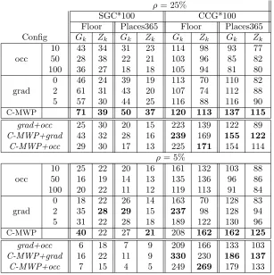
ρ= 25%

SGC*100 CCG*100

Floor Places365 Floor Places365 Config Gk Zk Gk Zk Gk Zk Gk Zk

10 43 34 31 23 114 98 93 77

occ 50 28 38 22 21 103 96 85 82

100 36 27 18 18 105 94 81 80

0 46 24 39 19 113 70 110 82

grad 2 61 31 43 20 107 74 112 88

5 57 30 44 25 116 88 116 90

C-MWP 71 39 50 37 120 113 137 115

grad+occ 25 30 20 15 223 139 122 89

C-MWP+grad 43 32 28 16 239 169 155 122

C-MWP+occ 29 30 17 13 225 171 154 114

ρ= 5%

10 25 22 20 16 161 132 103 88

occ 50 16 19 14 13 135 136 96 86

100 20 22 11 12 119 113 91 84

0 18 22 26 14 163 70 128 83

grad 2 35 28 29 15 237 98 128 94

5 31 22 28 18 189 122 130 96

C-MWP 40 22 27 21 208 162 162 125

grad+occ 6 18 7 9 209 166 133 103

C-MWP+grad 16 22 11 9 330 230 186 137

C-MWP+occ 7 15 4 5 249 269 179 133

Table 1: Average SCG and CCG (*100) for individual masks withρ= 25% and 5%. C-MWP performs best (bold) in almost all datasets, base image kernels, andρvalues. The intersection of all pairs of importance functions were also tested. Bold values show that CCG is higher for the pairs than for the best single most important region. For the pairs of functions, patch size foroccis 10 and dilation forgrad is 5.

5

Experiments

We performed experiments on two different datasets and the three importance functions. We first describe our datasets and the corresponding CNNs. Then, we present our experiments for evaluating the different important functions using our proposed metrics. Finally, we use our metrics and the datasets to compare the accuracy of the individual importance functions, and to the sets of features those importance functions agree on.

5.1

Datasets and Classifiers

We chose a scene recognition task because it is challenging for a person to identify which part of an image is most important to classification, compared to object detection tasks in which the object within the image should be most important. We expect subjective analysis of scene recognition visualizations to be less consistent because there are many areas or other aspects of the image that may affect scene classification.

challenging to determine which floor it is currently on. We collected the Building-Floor dataset in one of our buildings. Each image contains the scene just outside the elevator from six different floors of the building. The goal of the classifier trained on this dataset is to recognize the floor the image belongs to.

For each of the floors in the building, ten images were taken at specific locations outside the elevators where our robot stops, with slight variation in position. To simplify the analysis, all the images were taken at the same time of the day, and the effects of people moving around in the building are not considered. The training data consists of three images, and the remaining seven images form the testing dataset.

In order to classify the floor for each image, we chose to use a CNN based on Siamese architecture [4], because it has been shown to perform well in one-shot learning problems [5]. Our training network of nine layers followed AlexNet [6] with an input size ofN=227x227, in a modified Siamese architecture proposed in Sun et al. [11], Zheng et al. [17], which combined the identification– Softmax, and the verification loss– Contrastive, for better performance. We combined identification and verification loss with a pre-trained network to reduce overfitting which could happen when the complexity of network is higher than that of the data. During training, the first seven layers of our network were initialized from Places205-AlexNet which was trained in the Places205-Standard dataset and provided by the authors [18]. The remaining two layers were trained from scratch. During training, the contrastive loss was utilized in the eighth layer which is a dense layer of 1000 units, while the softmax loss was employed in the ninth layer. During testing, our network was able to classify all the images in the dataset correctly.

Places365-Standard. The Places365-Standard dataset [19] contains indoor and outdoor images from 365 categories. We used the Places365-AlexNet model with an input size of

N=227x227, provided by the authors, which was trained using∼1.8 million images. For testing, 200 random images were selected from the dataset without any other consideration like ground truth label.

5.2

Experimental Procedure

The three importance functions each required chosen parameters. For occ, the heat map is a function of the size of the occluding patches. For our evaluation, we varied the size of the occluding patches∈ {10,50,100} pixels. grad’s heat map H is of high entropy, so we dilate the raw heat map 0, 2, and 5 times with a 3x3 kernel. Dilating smoothens the heat map and improves the continuity of important regions as shown in Figure2(a). ForC-MWP, we use H

from thepool2 layer for both of the networks as we lose the spatial accuracy at higher layers. For ourC-MWP implementation, we used the source code provided by the authors.

Given the heat maps generated by each importance function, we then created the binary masks using simple thresholding to ensure that ρ% (ρ = 5 and 25) of the top features are consistent across tests. To create the base images, we used two different techniques - a Gaussian kernelGk of size 17x17 for creating the blurred base images and a zero kernelZk to substitute black for the non-important pixels. In order to create the accurate hybrid image, we grow the regions of the mask using a 3x3 dilate operation. When testing the common features in agreement between importance functions, we evaluated all pairs on both datasets, namely

grad+occ, C-MWP+grad, andC-MWP+occ. For the experiments in agreement with occ, we have fixed the patch size to be 10, and forgrad, the number of dilating operations is 5.

During the experiments, the images wherep(I =y|w)−p(IK =y|w) andp(IM,k=y|w)−

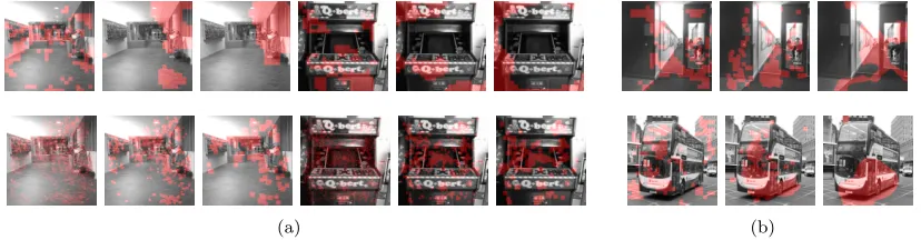
(a) (b)

Figure 2: (a) The image masks for the (top) occ importance function and (bottom) grad

importance function generated with the parameters ρ=25% and with dilation = {0, 2, 5} respectively for one image from the Building-Floor dataset (left three images) and one image from the Places365 dataset belonging to the classamusement station (right three images). (b) A side by side comparison of occ(patch size = 10),grad(dilation = 5), andC-MWPrespectively on an image from the Building-Floor and the Place365 dataset (ρ=25%).

belonging to the classnight, using a zero kernel Zk will make it the best image for the class. In both datasets less than 5% of the images violates this assumption. Although in our dataset and for the kernels we used, the number of images not obeying this assumption is small, there might be a dataset for which our kernel could result in a greater number of violations. In those cases we can opt to use a different kernel. Additionally, some images were omitted to fulfill a specific test condition. During CCG calculation, for example, we ignored the images where the

M had to be grown more than 50 times in order to avoid growing the mask too much beyond the original mask. In practice, this was an issue for some test images withρ=5%, about 5% of the test images were omitted from each dataset with this condition.

6

Results And Discussion

Evaluating Importance Functions. In total, 38 and 180 images were used for testing in Building-Floor and Place-365 dataset respectively. The quantitative results of the evaluation of the individual importance function’s masks are shown in Table1. The masks obtained from varying the respective parameters foroccandgradon one image from each dataset are shown in Figure2(a)(top) and2(a)(bottom). Forocc, we find that the patch size of 10 on average performs better than that of 50 which is better than 100. occ rates all pixels covered by large occlusion patches as important when only a small area under the occlusion may actually be important. A patch size of 10 occludes smaller regions of important features and is more concise, and hence better captures what the network has learned. Forgrad, dilating the important region 2 or 5 times performs as well or better than not dilating the heat map. When the important regions have high entropy (e.g., 0 dilations), the hybrid image is not informative for the classifier.

A side by side comparison of the mask obtained for occ with patch size=10, grad with number of dilations=5, andC-MWP are shown in Figure 2(b). Among the three, on average

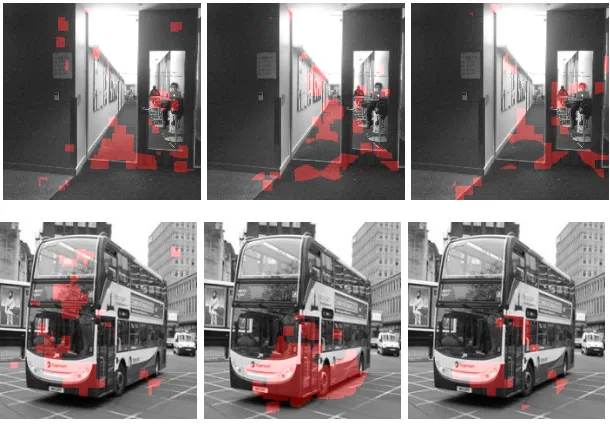
Figure 3: A side by side comparison of the three pairs of importance functions (grad+occ, C-MWP+grad, andC-MWP+occrespectively) on an image from the Building-Floor dataset (top) and the Place365 dataset (ρ=25%) (bottom).

metrics consistently find that the C-MWP importance function outperforms the others across a random sample of scenes, demonstrating the robustness of our metrics to accommodate for large variations in features and image labels.

Effect Of Varying Parameters. We varied ρ= 5% and 25% as the size of the mask. We found thatSCGmetric was higher for larger masks andCCGwas higher for smaller ones. This indicates that when the percentage of the image retained decreases so does the size of important regions leaving a more concise area. However, the larger mask size does not increase the mask proportionately. CCG finds that the smaller area is sufficient for achieving “high enough” accuracy while SCG values the higher accuracy achieved with more pixels. Selecting values ofρfor future evaluations of importance functions should take this trade-off into account. CCG on average dilates the accurate mask for 10 (ρ= 5%) and 6 iterations (25%) respectively. Although we did not analyze kernel parameters extensively, our initial experiments showed that changing the kernel parameter did not significantly affect the metrics nor the relative ranking among the three importance functions.

Agreement Between Importance Functions. We then analyzed the features that were in agreement or in common between different importance functions (results shown in Table1

and the masks are visualized in Figure3). The in-common features resulted in higher average CCG values than those computed using individual important features, as predicted. However, the in-common average SCG values are lower than the individual ones, because SCG considers only the amount of information gained and not the density or conciseness of the features like CCG.

other features as well. Subjectively, we agree that the glass door is the most discriminative feature of that image and of the floor because it is the only floor with a glass door. Similarly, in the image from the Places365 dataset, in-common importance masks capture only the bus while the individual functions capture additional features.

Among all combinations of importance functions that we tested for agreement, C-MWP+grad performs best, beating C-MWP+occ by a small margin. Both C-MWP+grad

andC-MWP+occoutperformgrad+occby a large margin. BecauseC-MWPperforms the best individually followed bygrad, it makes sense that comparing the features in agreement would also result in better performance. We also conducted experiments to find the intersection of all three importance masks and observed that the CCG scores were on average higher and SCG scores were on average lower than the ones of common importance masks for the other two importance functions.

We conclude that finding common features from different importance functions result in a more concise region of important features, which can be beneficial for preventing information overload to humans for visualization as well as determining the most discriminative pixels for classification.

Quantitative vs Qualitative Evaluation. Finally, we compared our metrics to those referred in prior findings based on subjective results on object recognition tasks. Our metrics found thatC-MWP outperforms the other two by a significant margin, followed bygrad and thenocc. This resultmatches the conclusion in Zhang et al. [16] which comparesC-MWP and

gradqualitatively (based on subjective human evaluation) and shows that the former is able to produce better localization of objects.

However, this may not necessarily always be the case that our objective metrics match the subjective results. For example, if the classifier uses pixels that are different from those that a human would find important, then the objective metrics will reveal different important regions as the best compared with those found using subjective metrics. We emphasize that our metrics capture the features that the DNN actually uses to classify, and therefore the direct correlation or comparison to subjective approaches is not necessarily possible for all situations.

7

Conclusion

Prior work to evaluate regions of images that are most discriminative for classification has been largely subjective, depending on humans to rate visualizations. In this work, we contribute two metrics – SCG and CCG – to address the need for an objective measure to assess the quality of different feature importance measures. The principle behind both metrics is to compare the proportion of the classifier accuracy that is attributed to the important features identified by the corresponding importance functions. Our CCG metric also takes into account the conciseness of the region and requires the classifier to classify the image accurately.

References

[1] Yuri Y Boykov and M-P Jolly. Interactive graph cuts for optimal boundary & region segmentation of objects in nd images. InComputer Vision, 2001. ICCV 2001. Proceedings. Eighth IEEE International Conference on, volume 1, pages 105–112. IEEE, 2001.

[2] Mikio L Braun, Joachim M Buhmann, and Klaus-Robert M ˜Aˇzller. On relevant dimensions in kernel feature spaces. Journal of Machine Learning Research, 9(Aug):1875–1908, 2008.

[3] Leo Breiman. Random forests. Mach. Learn., 45(1):5–32, October 2001. ISSN 0885-6125. doi: 10.1023/A:1010933404324. URLhttps://doi.org/10.1023/A:1010933404324.

[4] J. Bromley, I. Guyon, Y. LeCun, E. S¨ackinger, and R. Shah. Signature verification using a siamese time delay neural network. In Proceedings of the 6th International Conference on Neural Information Processing Systems, pages 737–744. Morgan Kaufmann Publishers Inc., 1993.

[5] G. Koch, R. Zemel, and R. Salakhutdinov. Siamese neural networks for one-shot image recognition. InICML Deep Learning Workshop, 2015.

[6] A. Krizhevsky, I. Sutskever, and G. Hinton. Imagenet classification with deep convolutional neural networks. InAdvances in neural information processing systems, pages 1097–1105, 2012.

[7] B. Lengerich, S. Konam, E. Xing, S. Rosenthal, and M. Veloso. Visual explanations for convolutional neural networks via input resampling. In Workshop on Visualization for Deep Learning, Thirty-fourth International Conference on Machine Learning, 2017.

[8] W. Samek, A. Binder, G. Montavon, S. Lapuschkin, and K. M¨uller. Evaluating the visual-ization of what a deep neural network has learned. IEEE Transactions on Neural Networks and Learning Systems, 2016.

[9] R. Selvaraju, A. Das, R. Vedantam, M. Cogswell, D. Parikh, and D. Batra. Grad-cam: Why did you say that? visual explanations from deep networks via gradient-based localization.

CoRR, abs/1610.02391, 2016.

[10] K. Simonyan, A. Vedaldi, and A. Zisserman. Deep inside convolutional networks: Visual-ising image classification models and saliency maps. InICLR Workshop, 2014.

[11] Y. Sun, Y. Chen, X. Wang, and X. Tang. Deep learning face representation by joint identification-verification. In Advances in neural information processing systems, pages 1988–1996, 2014.

[12] J.K. Tsotsos, S.M. Culhane, W.Y.K. Wai, Y. Lai, N. Davis, and F. Nuflo. Modeling visual attention via selective tuning. Artificial intelligence, 78(1-2):507–545, 1995.

[13] Shasha Xie, Yang Liu, and Hui Lin. Evaluating the effectiveness of features and sampling in extractive meeting summarization. In Spoken Language Technology Workshop, 2008. SLT 2008. IEEE, pages 157–160. IEEE, 2008.

[15] M. Zeiler and R. Fergus. Visualizing and understanding convolutional networks. In Euro-pean conference on computer vision, pages 818–833. Springer, 2014.

[16] J. Zhang, Z. Lin, J. Brandt, X. Shen, and S. Sclaroff. Top-down neural attention by exci-tation backprop. In European Conference on Computer Vision, pages 543–559. Springer, 2016.

[17] Z. Zheng, L. Zheng, and Y. Yang. A discriminatively learned CNN embedding for person re-identification. CoRR, abs/1611.05666, 2016.

[18] B. Zhou, A. Lapedriza, J. Xiao, A. Torralba, and A. Oliva. Learning deep features for scene recognition using places database. InAdvances in neural information processing systems, pages 487–495, 2014.

[19] B. Zhou, A. Khosla, A. Lapedriza, A. Torralba, and A. Oliva. Places: An image database for deep scene understanding. CoRR, abs/1610.02055, 2016.

[20] L. Zintgraf, T. Cohen, and M. Welling. A new method to visualize deep neural networks.