Value Balance and General Equilibrium Model

Issues

ISSN: 2146-4138

available at http: www.econjournals.com

International Journal of Economics and Financial Issues, 2017, 7(2), 485-491.

Value Balance and General Equilibrium Model

Truong Hong Trinh*

The University of Danang, University of Economics, Vietnam. *Email: [email protected]

ABSTRACT

This paper proposes a utility function with the incorporation of value and price, and develops a basic general equilibrium model with two conditions of market clearance and value balance. A joint value model is developed to conduct a value balance between firm profit and customer utility that is also a condition for market equilibrium. The simulation experiments are carried out to conduct the value balance between firm profit and customer utility, and the general equilibrium of the economy with economic policies. The study provides key evidence on the value balance between firm profit and customer utility that creates a new paradigm for further researches on partial equilibrium and general equilibrium.

Keywords: Value Concept, Utility Function, Joint Value, Value Balance, General Equilibrium

JEL Classifications: C61, C68, D46, D50

1. BACKGROUND

The concept of value has a very long history in economic and philosophical thought that attempt to explain two meanings of value: Value-in-use and value-in-exchange. The difference between value-in-use and value-in-exchange is important because it forms the base of value theories. Classical economics relies on the labor theory of value, which is an objective theory of value. It held that the value of the good come from, or is based on, the amount of labor spent producing that good or gone into bring it to market for exchange (value-in-exchange). This classical approach included the work of Smith (1776) and Ricardo (1821). Neoclassical economics relies on the utility theory of value, which is a subjective theory of value. It held that utility is measure of value. This stems from a subjective valuation of worth of the good by an economic agent (value-in-use). This neoclassical approach intended to conceptualize utility and construct a theory of price in keeping with the utilitarianism of Bentham (1789) and Dupuit (1844). Later, the new tool of marginal analysis as a means of understanding value, in which value would depend on the utility the buyer expects to receive, is developed by Jevons (1871) and Menger (1871).

Value concept plays a crucial role in determining relationship between demand and supply in markets, and resource allocation between firms and customers. Walras (1874) and Marshall (1890)

argued that both supply (cost of production) and demand (utility) are interdependent and mutually determinant of each other’s values. While Marshall (1890) developed his analysis to explain value in terms of supply and demand. Walras (1874) created his theoretical model of general equilibrium as a means of integrating both the effects of the demand and supply side forces in the whole country. Walrasian general equilibrium prevails when supply and demand are equalized across all of the interconnected markets in the economy. Based upon the theoretical base and the general equilibrium developed by Arrow and Debreu (1954), contemporary economists have attempted to developed general equilibrium model to study how resources are effectively allocated with the market mechanism.

of commodities and resources, zero profit condition assumes that all the firms are competitive and cannot earn excess profits (Hosoe et al., 2010). Due to subject to zero profit condition, the general equilibrium problem maximizes customer utility (or joint value) subject to production technology and market clearance conditions in quantity. As a result, the model can be applied to perfect competitive market in which both firms and customers are price taker. Meanwhile, the first order model (Lofgren et al., 2002) is used first order optimization conditions for production and consumption decisions that are driven by the maximization of customer utility and firm profit. In addition, Sue Wing (2009) approached both zero profit and first order conditions to maximize customer utility and firm profit.

Since these general equilibrium models use econometric techniques for equilibrium conditions that is not conducted the value balance between firm profit and customer utility, the first order conditions may find out local optimization solution for the general equilibrium model. The value balance is a basic condition for market equilibrium that also provides global optimization solution for general equilibrium. For that reason, this paper explores the value concept and defines the utility function with incorporation of value and price. A joint value model is developed to conduct the value balance between firm profit and customer utility. In addition, the value balance approach is used to conduct the general equilibrium of the economy.

2. VALUE BALANCE

In economics, concepts of value, utility, and price are important in the theory of value. A well-known neoclassical economist, Marshall, defined value as the equilibrium price formed when the marginal cost equaled the marginal utility (Deane, 1978). Utility, a concept from modern neoclassical economics, is defined as the satisfaction or pleasure derived by an economic agent (a person or a firm) from consuming a good or service, whereas marginal utility refers only to the utility obtained from the last unit consumed. The price consumers are willing to pay declines as the quantity purchased increases because of the diminishing returns obtained from additional purchases.

Most economists tried to make a clear distinction between value and price of a good or service. Baier and Rescher (1966) offered a broader definition such as “value is the capacity of a good, service, or activity to satisfy a need or provide a benefit to a person or legal entity.” Value is something which is perceived and evaluated at the time of consumption (Wikström, 1996; Woodruff and Gardial, 1996; Vargo and Lusch, 2004; Grӧnroos, 2008). There is a common understanding that value is created in the users’ processes as value-in-use (Grönroos, 2011). Since value-in-use (value) is more appreciate guide to well-being than value-in-exchange (price), should economists use the law of diminishing marginal utility to explain demand curve. In fact, the neoclassical utility concept is the same as the contemporary value concept. Thus, it needs to redefine the value concepts and theory of value should be constructed upon a law of diminishing marginal value (Trinh, 2014a). The theory of value not only interprets relationship between value and price, but also redefines the utility concept in this relationship. Based

on this theoretical base, the utility function is defined with the incorporation of value, price (Trinh et al., 2014) as follows.

TU = u×Q = (v−p)×Q = TV−TR (1)

Where, v, p, and u are unit value, unit price, and unit utility, respectively. TV, TR, and TU are total value, total revenue, and total utility, respectively.

From the value creation perspective, the value creation system involves three processes of production, exchange, and consumption as in Figure 1.

In firm perspective, the firm takes on the role of value facilitator, and also joins the customer’s value creation as a value co-creator. Firm’s production function is defined under the form of Cobb Douglas production function as follows:

Q = f K , L

(

S S

)

= A × KS SS × LSS

α β ₍₂₎

Where, Q is total output of production. A_S is firm’s total factor productivity. K_S and L_S are firm capital and firm labour, respectively. α_S, β_S are the output elasticities of production input factors.

By using the least-cost combination of production inputs, firm’s cost function (TC_S) can be determined as a function of output, depending on input prices and the parameters of the firm’s production function as follows:

TC_S = K_S×w_KS+L_S×w_LS (3)

Where, TC_S is firm’s total cost, w_KS and w_LS are unit costs of firm capital and firm labor, respectively.

Firm’s profit function is determined by the following formula.

Π = TR−TC_S = p×Q−K_S×w_KS-L_S×w_LS (4)

Where, Π is firm profit and TR is total revenue (TR = p×Q).

In customer perspective, the customer is always a value creator. The customer also takes part in the firm’s production process as a co-producer. Since the value is created in the consumption process, customer capital (K_D) and customer labor (L_D) are added

Figure 1: Value creation perspective

in the consumption function (Trinh, 2014a; Trinh, 2014b) as follows:

Q = f K , L

(

_{D D}

)

=A × K_{D D}αD× Lβ_DD (5)

Where, Q is total output of consumption. A_D is customer’s total factor productivity. α_D, β_D, are the output elasticities of consumption input factors.

By using the least-cost combination of consumption inputs, customer’s cost function (TC_D) can be determined as a function of output, depending on input prices and the parameters of the customer’s consumption function as follows:

TC_D = K_D×w_KD+L_D×w_LD (6)

Where, TC_D is customer’s total cost, w_KD and w_LD are unit costs of customer capital and customer labor, respectively.

Customer’s utility function is determined by the following formula.

U = TU−TC_D = (v−p)×Q−K_D×w_KD−L_D×w_LD (7)

Where, U is customer utility and TU is total utility (TU = u×Q = [v−p]×Q).

From the value creation perspective, value is created in the consumption process, both firm cost and customer cost have to consider in value creation systems. The joint cost function and the joint value function are determined as follows:

TC = TC_S+TC_D = K_S×w_KS+L_S×w_LS+K_D×w_KD+L_D×w_LD (8)

V = Π+U = v×Q−(K_S×w_KS+L_S×w_LS+K_D+w_KD+L_D×w_LD)

= TV−TC (9)

Where, V is joint value, TV is total value (TV = v×Q) and TC is total joint cost.

From the above formulas, the joint value is driven by use (v), but the value allocation is monitored by value-in-exchange (p). When the firm gets access to join the customer’s value creation as value co-creator, value-in-use (v) is co-created upon firm resources and customer resources. Meanwhile, value-in-exchange (p) has an impact to levels of output (Q) and a value balance between firm profit (П) and customer utility (U). While the profit approach provides a solution for profit maximization (П_Max), the utility approach provides a solution for utility maximization (U_Max). The value approach is to maximize a joint value (V_Max = П+U), which provides an optimal solution for the value balance between firm profit (П) and customer utility (U).

The joint value model:

Max V=

v ×Q K ×w +L ×w +K ×w +L ×w

j j Sj KSj Sj LSj

Dj KDj Dj LDj j=1

m  −



 [ _] _

∑

∑

(10)

Subject to

v_j = f(Q_j), Ɐ_j = 1…m (11)

p_j = f(Q_j), Ɐ_j = 1…m (12)

Q = A ×KSj Sj Sj ×L , =1..mSj

Sj Sj

α β _{∀ (13)}

Q_Dj= A ×K_Dj α_DjDj×Lβ_DjDj, ∀j=1..m (14)

Q_j = Q_Sj = Q_Dj, Ɐ_j = 1…m (15)

ⱯQ_Sj, Q_Dj, K_Sj, L_Sj, K_Dj, L_Dj Ɐ_j = 1…m

The objective function is to maximize the joint value of firm profit and customer utility as in equation 10. Market demand presents the relationship between value (v_j) and price (p_j) with their demand quantity (Q_j) that is shown under constraints of (11) and (12). Production technology and consumption technology are shown by constraints of (13) and (14). Market clearance imposes an equilibrated condition of demands and supplies. The joint value model provides a value balance solution that maximizes the joint value (V) of firm profit (П) and customer utility (U).

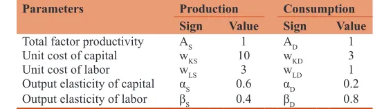
In order to conduct the value balance between firm profit and customer utility, a simulation experiment is carried out via a hypothetical system with a single offering (j = 1), in which the production function and consumption function are assumed to be a well-defined function. Table 1 presents parameters of the value creation system.

Demand function indicates relationship between value (v) and price (p) with their quantity demand (Q) given as follows:

Value demand: v= 3 10Q+29

−

Price demand: p= 1 5Q+21

−

Table 2 presents the simulation results for three approaches. The profit approach provides the optimal solution for profit maximization (П_Max = 98.80), and the utility approach provides the optimal solution for utility maximization (U_Max = 88.37). The value approach provides the optimal solution of joint value maximization (V_Max = П+U = 183.41), which provides the value balance between firm profit (П = 97.55) and customer utility (U = 85.86). Since there exist a tradeoff between the profit approach and the utility approach, the value approach provides a value balance between these two approaches that maximizes the joint value.

Table 1: Parameters of the value creation system

Parameters Production Consumption

Sign Value Sign Value

Total factor productivity A_S 1 A_D 1

Unit cost of capital w_KS 10 w_KD 3

Unit cost of labor w_LS 3 w_LD 1

Output elasticity of capital α_S 0.6 α_D 0.2

3. GENERAL EQUILIBRIUM MODEL

The general equilibrium model provides a comprehensive macroeconomic framework to describe market-oriented economies. The structure of the economy has three main components: Customers, producers, and markets as in Figure 2. Customers (householders) decide demand of commodities in commodity market and supply their resources in resource market to maximize their utility. Producers (Firms) decide demand of production inputs in resource market and supply their production outputs in commodity market to maximize their profits. These demands and supplies are equilibrated by resource allocation and market adjustment.

In the real economy, the economy is expanded with economic policies, such as international trade (NX), tax or subside (T), government expenditure (G), capital investment (I), and capital depreciation (D). Under conditions of market clearance and value balance, the basic general equilibrium model is developed with main assumptions as follows:

1. Householders (customers) consume m offerings (products or services) with the same preference or consumption parameters.

2. Firms (producers) provide m identical offerings with the same production parameters.

3. Both customers and firms take part in the offering process, in which the joint value function involves both firm inputs and customer inputs.

4. Demand function is well-defined function that includes both value demand and price demand.

5. International trade (NX), tax or subside (T), government expenditure (G), capital investment (I), and capital depreciation (D) are given parameters in the model.

In order to conduct general equilibrium under the value balance approach, the simulation experiment is carried out on the hypothetical economy with m offerings (products and services). Firms produce offerings j (j = 1…m) by using firm capital (K_Sj) and firm labor (L_Sj). Householders consume offering j (j = 1…m) by adding customer capital (K_Dj) and customer labor (L_Dj). The demand function of offering j is defined as follows:

Value demand: v_j = f(Q_j) (16)

Price demand: p_j = g(Q_j) (17)

Market clearance condition imposes a condition to equilibrate total supply (Q_Sj) and total demand (Q_Dj) for all offerings (j = 1…m).

Market clearance: Q_j = Q_Dj = Q_Sj (18)

Production function (Q_Sj) and consumption function (Q_Dj) of offering j are given as follows:

Production function: Q = A ×K_{Sj Sj Sj}αSj×Lβ_SjSj (19)

Consumption function: Q =A ×K_{Dj Dj Dj}αDj×Lβ_DjDj (20)

Total profit function (П) and total customer utility (U) of all offerings in the economy are determined as follows:

Profit function:

∏= p ×Q_j K ×W L ×W T

j 1 m

Sj Sj KSj j=1

m

Sj LSj j=1

m

j j=1

m

−

∑

−

∑

−

∑

−

∑

(21)

Where, T_j is tax or subside of the offering j (j = 1…m).

Utility function:

U= v_j p ×Q_j K ×W L ×W

j 1 m

Dj Dj KDj j=1

m

Dj LDj j=1

m

−

(

)

− −

−

∑

∑

∑

(22)

Since joint value (V) is sum of customer utility (U) and firm profit (П) and market clearance is satisfied as in equation 18, the formula of the joint value can be expressed as:

V= v ×Q K ×W L ×W

K ×W L ×W

j Sj j=1

m

Sj KSj Sj LSj j=1

m

Dj KDj Dj LDj

∑

−

∑

(

−

)

−

(

−

)

jj=1 m

j j=1

m

T

∑

−

∑

₍₂₃₎

The following general equilibrium model is to maximize the joint value under two conditions of market clearance and value balance.

The basic general equilibrium model: Table 2: Simulation results of the system

Approaches Profit

maximization maximizationUtility maximizationValue

K_S 16.15 21.60 17.97

L_S 35.89 48.00 39.92

K_D 3.04 4.07 3.39

L_D 36.53 48.86 40.64

Q 22.23 29.73 24.73

v 22.33 20.08 21.58

p 16.55 15.05 16.05

П 98.80 87.54 97.55

U 82.74 88.37 85.86

V 181.54 175.91 183.41

Max V = Π+U (24)

Subject to

v_j = f(Q_j) Ɐ_j = 1…m (25)

p_j = g(Q_j) Ɐ_j = 1…m (26)

Q_j = Q_Dj = Q_Sj Ɐ_j = 1…m (27)

Q = A ×K_{Sj Sj Sj}αSj×Lβ_SjSj∀=1..m (28)

Q =A ×K_{Dj Dj Dj}αDj×Lβ_DjDj∀=1..m (29)

Π= p ×Q K ×W L ×W

T =1..m

j j-1 m

Sj Sj KSj j=1

m

Sj LSj j=1

m

j j=1

m

∑

∑

∑

∑

− −

− ∀ (30)

U= v_j p ×Q_j K ×W L ×W =1..m

j 1 m

Dj Dj KDj j=1

m

Dj LDj j=1

m

−

(

)

− − ∀

−

∑

∑

∑

(31)

ⱯQ_Sj, Q_Dj, K_Sj, L_Sj, K_Dj, K_Dj Ɐ_j = 1…m

Notations:

Indices:

j: Index of offering (j = 1…m).

System parameters:

A_Sj: Total factor productivity of production of offering j A_Dj: Total factor productivity of consumption of offering j w_KSj: Unit cost of firm capital of offering j

w_LSj: Unit cost of firm labor of offering j w_KDj: Unit cost of customer capital of offering j w_JDj: Unit cost of customer labor of offering j α_Sj: Output elasticity of firm capital of offering j β_Sj: Output elasticity of firm labor of offering j α_Dj: Output elasticity of customer capital of offering j β_Dj: Output elasticity of customer labor of offering j.

Policy parameters:

T_j: Tax or subside impose on offering j Q_NXj: Net export output of offering j

Q_Gj: Government expenditure output of offering j I_j: Capital investment of offering j

D_j: Capital depreciation of offering j.

Variables:

Q_Sj: Total production output of offering j Q_Dj: Total consumption output of offering j K_Sj: Total firm capital of offering j

L_Sj: Total firm labor of offering j K_Dj: Total customer capital of offering j L_Dj: Total customer labor of offering j.

The simulation experiment assumes that the hypothetical economy has only one offering (j = 1). Parameters of the economy are given in Tables 3 and 4.

In order to study how the economy allocates resources under market adjustments of value and price, market demand of the offering j (j = 1) is given under the law of diminishing marginal value as follows (Table 5):

Value demand: v = 3 10Q +29

j − j

Price demand: p = 1 5Q +21

j − j

The expenditure approach measure gross domestic product (GDP) by using data on personal expenditure, capital investment, government expenditure, and net export. GDP using in the expenditure approach is the sum of personal expenditure (C), capital investment (I), government expenditure (G), and net export (NX). Table 6 shows the expenditure approach for GDP measurement of the economy.

GDP = C+I+G+NX (32)

The income approach measures GDP by summing up the incomes that firms pay householders for the resources they hire such as labor wage (Lw_LS), capital interest (Kw_KS), firm saving (S_F), capital depreciation (D), tax and subside (T). GDP using the income approach is the sum of personal expenditure (C), capital depreciation (D), total saving (S), tax and subside (T). Table 7 shows the expenditure approach for GDP measurement of the economy.

GDP = C+D+S+T (33)

Figure 3 illustrates the circular flow of income and expenditure. Householders receive capital interest (K_Sw_KS = 179.65) and labor wage (L_Sw_LS = 119.77) from the resource market, and make personal expenditure (C = 284.59) in the commodity market. Firms make capital investment (I = 10) and get capital depreciation (D = 20), government purchases commodities (G = 32.11), and the rest of the world purchases net export (NX = 80.27). Total saving

Table 3: System parameters of the economy

Offering j Production Consumption

Sign Value Sign Value

Total factor productivity A_Sj 1 A_Dj 1

Unit cost of capital w_KSj 10 w_KDj 3

Unit cost of labor w_LSj 3 w_LDj 1

Output elasticity of capital α_Sj 0.6 α_Dj 0.2

Output elasticity of labor β_Sj 0.4 β_Dj 0.8

Table 4: Policy parameters of the economy

Offering j Sign Value

Tax or subside T_j 30

Capital investment I_j 10

Capital depreciation D_j 20

Net export output Q_NXj 5

(S = 72.39) includes customer (householder) saving (S_C = 14.84) and firm saving (S_F = 57.55). Customer saving (S_C = 14.84) and firm profit (П = 67.55) would lend in the financial market, where government and the rest of the world would borrow to finance their deficits.

4. CONCLUSIONS

Theory of value encompasses all the theories within economics that attempt to explain why goods and services are priced as they are, how the value of goods and services come about. Neoclassical economists argue that value has origins in exchanged and used process and price is depended on its utility, in which the price consumers are willing to pay declines under the law of the diminishing marginal utility. Since value concept is more appreciate guide to well-being than price concept, the theory of value refines the relationship between value and price, in which the utility function is defined with the incorporation of value and price.

The joint value model is developed to conduct the value balance between firm profit and customer utility. The simulation experiments are carried out on the hypothetical system, in which both firm inputs and customer inputs are considered in the value creation system. The experimental result indicates that there exist the value balance between firm profit and customer utility, in which the value balance is also the basic condition for market equilibrium (Trinh, 2014a). Under the value balance approach, the simulation study is to conduct the general equilibrium of the economy with economics policies. The study result provides key evidence on the value balance between firm profit and customer utility. Moreover, the value balance approach creates a new paradigm for further researches on partial equilibrium and general equilibrium.

Table 5: Simulation results of the economy

Result Formula Value

Total output Q_j=Q_Cj+Q_Gj+Q_NXj 24.73

Unit price

p = 1 5Q +21

j − j

16.05

Unit value

V = 3 10Q +29

j − j

21.58

Firm profit

Π= p ×Q K ×W

L ×W T

j j-1 m

Sj Sj KSj

j=1 m

Sj LSj j=1 m

j j=1 m

∑

∑

∑

∑

−

− −

67.55

Customer

utility U= v p ×Q

K ×W L ×W

j j j-1 m

Dj

Dj KDj j=1

m

Dj LDj j=1

m

−

(

)

− −

∑

∑

∑

85.86

Joint value V = Π + U 153.41

Personal expenditure

m j Cj j=1

C= p ×Q

∑

284.59

Government expenditure

m j Gj j=1

G= p ×Q

∑

32.11

Customer

saving S = K ×w +L ×w

p ×Q

C Sj KSj Sj LSj

j=1 m

j Cj j=1

m

(

)

−

∑

∑

14.84

Firm saving

S = +_F I_j D j=1

m

j j=1

m

Π

∑ ∑

− 57.55

Total saving S=S_C+S_F 72.39

Sources: These above formulas are adapted from Trinh (2014b)

Table 6: The expenditure approach for GDP measurement

Items Symbol Quantity Price Amount

Personal expenditure C 17.73 16.05 284.59

Capital investment I - - 10

Government expenditure G 2 16.05 32.11

Net export NX 5 16.05 80.27

GDP GDP 406.97

GDP = C + I + G + NX = 284.59 + 10 + 21.11 + 80.27 = 406.97

REFERENCES

Arrow, K.J., Debreu, G. (1954), Existence of an equilibrium for a competitive economy. Econometrica, 22(3), 265-290.

Baier, K., Rescher, N., editors. (1966), What is value? An analysis of the concept. Value and the Future: The Impact of Technology Change on American Values. New York: The Free Express. p33-67. Bentham, J. (1789), An Introduction to the Principles of Morals and

Legislation. Oxford: Clarendon Press (1907).

Deane, P. (1978), The Evolution of Economic Ideas. London: Cambridge University Express.

Dupuit, J. (1844), De l’utilite’ et de sa Mesure, La Riforma Sociale (1933). Italy: Torino.

Grönroos, C. (2011), A service perspective on business relationships: The value creation, interaction and marketing interface. Industrial Marketing Management, 40(2), 240-247.

Grӧnroos, C. (2008), Service logic revisited: Who creates value? And who co-creates? European Business Review, 20(4), 298-314.

Grӧnroos, C., Voima, P. (2012), Making Sense of Value and Value

Co-creation in Service Logic. Helsinki, Finland: Hanken School of Economics.

Hosoe, N., Gasawa, K., Hashimoto, H. (2010), Textbook of Computable General Equilibrium Modeling: Programming and Simulations. London: Palgrave Macmillan.

Jevons, S.W. (1871), Theory of Political Economy. London: Macmillan (1970).

Lofgren, H., Harris, R.L., Robinson, S. (2002), A Standard Computable General Equilibrium (CGE) Model in GAMS. Washington, DC: International Food Policy Research Institute (IFPRI).

Marshall, A. (1890), Principles of Economics. London: Macmillan. Menger, C. (1871), Principles of Economics. Germany: Braumüller. Ricardo, D. (1821), On the Principles of Political Economy and Taxation.

London: John Murray.

Smith, A. (1776), The Wealth of Nations. New York: The Modern Library (1937).

Sue Wing, I. (2004), Computable General Equilibrium Models and Their Use in Economy-Wide Policy Analysis. MIT Joint Program on the Science and Policy of Global Change.

Sue Wing, I. (2009), computable general equilibrium models for the analysis of energy and climate policies. In: Evans, J., Hunt, L.C., editors. International Handbook on the Economics of Energy. Cheltenham: Edward Elgar. p332-366.

Trinh, T.H. (2014a), A new approach to market equilibrium. International Journal of Economic Research, 11(3), 569-587.

Trinh, T.H. (2014b), Value concept and economic growth model. Journal of Economic and Financial Studies, 2(6), 62-71.

Trinh, T.H., Kachitvichyanukul, V., Khang, D.B. (2014), The co-production approach to service: A theoretical background. Journal of the Operational Research Society, 65(2), 161-168.

Vargo, S.L., Lusch, R.F. (2004), Evolving to a new dominant logic for marketing. Journal of Marketing, 68(1), 1-17.

Walras, L. (1874), Elements of Pure Economics. London: George Allen and Unwin (Reprinted: 1954).

Wikström, S. (1996), The customer as co-producer. European Journal of Marketing, 30(4), 6-19.

Woodruff, R.B., Gardial, S. (1996), Know Your Customers – New Approaches to Understanding Customer Value and Satisfaction. Cambridge, MA: Blackwell Business.

Table 7: The income approach for GDP measurement

Items Symbol Quantity Price Amount

Capital interest K_Sw_KS 17.97 10 179.65

Labor wage L_Sw_LS 39.92 3 119.77

Firm saving S_F - - 57.55

Capital depreciation D - - 20

Tax and subside T - - 30

GDP GDP 406.97