Lee06

Dynamic Characterization of Cluster

Structures for Robust and Inductive

Support Vector Clustering

Jaewook Lee,

Member

,

IEEE

, and Daewon Lee

Abstract—A topological and dynamical characterization of the cluster structures described by the support vector clustering is developed. It is shown that each cluster can be decomposed into its constituent basin level cells and can be naturally extended to an enlarged clustered domain, which serves as a basis for inductive clustering. A simplified weighted graph preserving the topological structure of the clusters is also constructed and is employed to develop a robust and inductive clustering algorithm. Simulation results are given to illustrate the robustness and effectiveness of the proposed method.

Index Terms—Clustering, kernel methods, support vector machines, inductive learning, dynamical systems.

Ç

1

I

THE support vector clustering (SVC) methods [1], [7], [8] are recently emerged algorithms to characterize the support of a high dimensional distribution inspired by the support vector machines (SVMs) [2], [9] and have been successfully applied to solve some difficult and diverse clustering or outlier detection problems [1], [3], [6], [8]. These methods map data points by means of a kernel to a high dimensional feature space and find a sphere with minimal radius that contains most of the mapped data points in the feature space. This sphere, when mapped back to the data space, can separate into several components, each enclosing a separate cluster of points as in [1]. They have some advantages over other clustering algorithms for their ability to generate cluster bound-aries of arbitrary shape and to deal with outliers by employing a soft margin constant that allows the sphere in feature space not to enclose all points, although some model selection problems arise from the difficulties in choosing a suitable kernel parameter [1], [6]. In this paper, we explore the topological structure of the clusters generated by the SVC utilizing an associated dynamical system and show that each cluster can be decomposed into its constituent (dynamically invariant) sets, the so-called basin level cells, of the constructed system. This decomposition not only facilitates the cluster labeling of each sample data point, but also makes it possible to assign cluster labels to unknown data points, thereby providing a way to partition the whole data space into separate clustered domains for inductive clustering.

We also construct a simplified weighted graph preserving the topological structure of the clusters by introducing the concepts of an adjacency and a transition point between basin cells. The constructed graph is applied to developing a robust method to differentiate between the decomposed basin level cells, which is crucial for the correct cluster labeling of the sample data points. The proposed method is shown through simulation to improve and extend the clustering ability of the traditional SVC algorithms.

2

A R

S

V

C

The support vector clustering methods build cluster boundaries which enclose the data points by computing a set of contours generated by a so-called trained kernel support function. Following

the derivation of [1], [8] in this section, we construct a trained kernel support function as follows: Letfxig X be a given data set of N points, with X <n_{, the data space. Using a nonlinear} transformationfromX to some high dimensional feature space, we look for the smallest enclosing sphere of radiusRdescribed by the constraints

kðxjÞ ak2R2þj; ð1Þ

whereais the center. Introducing the Lagrangian with penalty term

L¼R2X j

ðR2_þ

j kðxjÞ ak2Þj

X

j

jjþC

X

j j;

the solution of the primal problem (1) can be obtained by solving its dual problem:

max W¼X j

ðxjÞ2 j

X

i;j

ijðxiÞ ðxjÞ

subject to 0jC;

X

j

j¼1; j¼1;. . .; N:

ð2Þ

Only those points with0< j< Clie on the boundary of the sphere and are called support vectors (SVs). Points withj¼Clie outside the boundaries and are called bounded support vectors (BSVs).

The trained kernel support function (TKSF), defined by the radial distance of the image ofxfrom the sphere center, is then given by

fðxÞ ¼R2ðxÞ ¼ kðxÞ ak2

¼Kðx;xÞ 2X j

jKðxj;xÞ þ

X

i;j

ijKðxi;xjÞ; ð3Þ

where the Gaussian kernelKðxi;xjÞ ¼ðxiÞ ðxjÞ ¼expðqkxi xjk2_Þ

with width parameterqis used. One distinguishing feature of the trained kernel support function is that cluster boundaries can be constructed by a set of contours that enclose the points in data space given by fx:fðxÞ ¼rg, wherer¼R2_{ðxiÞfor any support} vectorxi. (See Fig. 2a.)

Specifically, the level set, LfðrÞ, of fðÞ is decomposed into several different clusters:

LfðrÞ ¼ def

fx:fðxÞ rg ¼C1[ [Cp; ð4Þ

where theCi; i¼1;. . .; pare different clusters corresponding to the disjoint connected sets and p is the number of clusters determined byR2_ðÞ.

3

C

D

Since the clusters generated by the SVC correspond to the connected components of the level setLfðrÞdescribed by (4), the cluster structure can be analyzed by exploring a topological property (e.g., connectedness) of the level sets. To characterize the topological property of the level setLfðrÞ, in this paper, we build a dynamical system associated with the trained kernel support function,f, and show that each connected component,Ci, ofLfðrÞ is exactly composed of dynamically invariant sets, the so-called basin level cells, of the constructed system. This decomposition will be shown to facilitate the cluster labeling of each sample data point and to extend the clusters to enlarged clustered domains that constitute the whole data space.

3.1 Dynamical System Formulation

Consider a (negative) gradient dynamical system associated with the trained kernel support function,f, described by

dx

dt¼ rfðxÞ: ð5Þ

The existence of a unique solution (or trajectory)xðÞ:< ! <n_for each initial conditionxð0Þis guaranteed since the functionfin (3) is twice differentiable and the norm ofrf is bounded [4]. A state

. The authors are with the Department of Industrial and Management Engineering, Pohang University of Science and Technology, Pohang, Kyungbuk 790-784, Korea. E-mail: {jaewookl, woosuhan}@postech.ac.kr. Manuscript received 10 July 2005; revised 22 Mar. 2006; accepted 22 Mar. 2006; published online 14 Sept. 2006.

Recommended for acceptance by J. Buhmann.

For information on obtaining reprints of this article, please send e-mail to: [email protected], and reference IEEECS Log Number TPAMI-0363-0705.

vectorxsatisfying the equationrfðxÞ ¼0is called anequilibrium

point(or critical point) of system (5). We say that an equilibrium

pointxof (5) ishyperbolicif the Hessian matrix offatx, denoted by r2_{fðxÞ, has no zero eigenvalues. Note that all the eigenvalues of} r2_{fðxÞare real since it is symmetric. A hyperbolic equilibrium point} is called 1) a (asymptotically)stableequilibrium point (or anSEP) if all the eigenvalues of its corresponding Hessian are positive, 2) an

unstableequilibrium point (or aUEP) if all the eigenvalues of its

corresponding Hessian are negative, or 3) asaddle pointotherwise. A hyperbolic equilibrium pointxis called anindex-ksaddle pointif its Hessian has exactlyknegative eigenvalues. A setKin<n_{is called a}

positively (negatively) invariant set of (5) if every trajectory of (5)

starting inKremains in a setKfor allt0(t0).

The next proposition states the complete stability and the positive invariance property of each cluster in (4) under process (5). Proposition 1 [6]. For a given trained kernel support function f,

suppose that for anyx02 <n, each connected component of the level

setLfðrÞ ¼ fx:fðxÞ rgis compact, wherer¼fðx0Þ. Then, (5) is

completely stable, i.e., every trajectory of (5) approaches one of the equilibrium points of (5). Furthermore, each connected component of

the level set LfðrÞ is positively invariant, i.e., if a point is on a

connected component ofLfðrÞ, then its entire positive trajectory lies

on the same component.

Remark.From the form of a Gaussian kernel, it can be shown that a trained Gaussian kernel support function f satisfies the condition of this proposition; that is, each connected component of the set fx:fðxÞ fðx0Þg is compact. Unless otherwise specified, in this paper, we will assume that the trained kernel support functionf satisfies this condition.

3.2 Cluster Decomposition

One important notion introduced in this paper is a basin cell and a basin level cell, which helps us to decompose the whole data space into several separate clustered domains.

Definition 1.1) Thebasin of attractionof an SEP,s, is defined as

AðsÞ:¼ fxð0Þ 2 <n_{: lim}

t!1xðtÞ ¼sg:

and the closure of the basinAðsÞ, denoted byAðsÞ, is called abasin cell.

The boundary of the basin cell defines thebasin cell boundary, denoted

by@AðsÞ. 2) The basin level set ofs, relative to a level valuer, is defined as the set of points in the level setLfðrÞthat converges toswhen (5) is

applied; that is,

BrðsÞ:¼ fxð0Þ 2LfðrÞ: lim

t!1xðtÞ ¼sg:

and the closure of the basin level setBrðsÞ, denoted byBrðsÞ, is called abasin level cell.

From a topological point of view,AðsÞandAðsÞare both connected and invariant [4]. We next present a result showing that each cluster can be decomposed into the basin level cells of its constituent SEPs.

Theorem 1.Letsi; i¼1;. . .; l be the set of all the stable equilibrium

points of system (5) in a (nonempty) level set LfðrÞ. Then the

following holds:

1. Each basin level cell is given by

BrðsiÞ ¼AðsiÞ \LfðrÞ

and is connected and positively invariant.

2. The level setLfðrÞis decomposed into the basin level cells;

that is,

LfðrÞ ¼ fx:fðxÞ rg ¼

[l

i¼1

BrðsiÞ: ð6Þ

3. Ifsik; k¼1;. . .; li is the set of all the stable equilibrium points in a clusterCi, then

Ci¼

[li

k¼1

BrðsikÞ: ð7Þ

Proof.

1. SinceAðsiÞandLfðrÞare both positively invariant, their intersection, i.e., the basin level cell

BrðsiÞ ¼AðsiÞ \LfðrÞ;

is also positively invariant. The connectedness of the basin level set can be proven in the same way as that of the basin of attraction except that the starting points are restricted to be in LfðrÞ [5]. Since the closure of a connected set is connected, the basin level cellBrðsiÞis connected.

2. By the complete stability property of system (5) from Proposition 1, we have<n_¼Sp

i¼1AðsiÞ, wheresi; i¼

lþ1;. . .; pis the set of all the stable equilibrium points outside the level setLfðrÞof system (5). SinceAðsiÞ \ LfðrÞ ¼ ;fori¼lþ1;. . .; p, we have

LfðrÞ ¼

[p

i¼1

ðAðsiÞ \LfðrÞÞ ¼[ p

i¼1

BrðsiÞ ¼[ l

i¼1

BrðsiÞ:

3. Since the level set LfðrÞ consists of several different clustersCias in (4), the result follows immediately. tu

Theorem 1 implies that, for any sample data pointx2LfðrÞ, there exists a corresponding SEP, saysi, such thatx2BrðsiÞand the cluster to which a data pointxbelongs is identical to the cluster to which its corresponding SEP,si, belongs. Therefore, the cluster labeling of each sample data point can be accomplished by identifying the cluster label of its corresponding SEPsi to which the data point converges by (5). (See Fig. 2a.)

Theorem 1 also serves as a basis to extend the clusters given in (4) to enlarged clusters as follows: Since any point in the basin cell AðsiÞenters into the basin level cell BrðsiÞ when (5) is applied, AðsiÞ, which is connected and invariant, can be considered a natural extension ofBrðsiÞ. Therefore, ifsik; k¼1;. . .; liis the set

of all the stable equilibrium points in a clusterCi, then the cluster Cican be extended to an enlarged clusterCiECigiven by

C_iE¼[ li

k¼1

AðsikÞ: ð8Þ

By the way, since the basinsAðsiÞare disjoint and the whole data space<n_{is composed of the basin cellsAðsi}

kÞ, the whole space is

partitioned into separate clustered domains, i.e.,

<n_¼CE

1 [ [C E

p: ð9Þ

Therefore, this extension provides us with a natural way to assign cluster labels to unknown data points, which is one distinguishing feature of our dynamical system approach in clustering.

4

C

C

S

which provides us with a robust way to differentiate between the SEPs that belong to different clusters.

4.1 Adjacency and Transition Point

Other important notions introduced in this paper are the adjacency and the transition point. Before giving these definitions, we present a result showing a dynamic relationship between a stable equilibrium point (SEP) and an index-one saddle point lying on its basin cell boundary.

Proposition 2 ([5]).Letsabe an SEP of (5). Then, there exists an

index-one saddle pointd2@AðsaÞsuch that the 1D unstable manifold1_(or

curve) Wu_{ðdÞ of d converges to another stable equilibrium point,}

saysb.

This result leads to the following definition:

Definition 2.Two SEPs,saandsb, are said to beadjacentto each other

if there exists an index-one saddle pointd2AðsaÞ \AðsbÞ. Such an

index-one saddle point, d, is called a transition point between sa

andsb.

Note that, in our definition, the existence of the transition point is necessary for the adjacency of two SEPs in addition to the condition that the two basin cells intersect. For example, in Fig. 2a, the basin cells Aðs6ÞandAðs8Þof two SEPs, s6 ands8, intersect (only one intersection point), but they are not adjacent to each other in terms of our definition since there does not exist a transition point between them. By contrast, two SEPs,s6ands7, are adjacent to each other since there exists a transition point between them.

We next derive a result showing that only the transition points are sufficient to determine whether two adjacent SEPs are in the same cluster.

Theorem 2.Letsi;sjbe any two adjacent SEPs of (5). IffðdÞ< rfor a

transition pointdbetweensi andsj, thensi andsjare in the same

cluster ofLfðrÞ.

Proof. Let d be a transition point between si andsj. Since d2 AðsiÞ \AðsjÞandfðdÞ< r, we have

d2AðsiÞ \AðsjÞ \LfðrÞ ¼BrðsiÞ \BrðsiÞ:

Since BrðsiÞ, BrðsiÞ, and their intersection are all connected, BrðsiÞ [BrðsiÞis connected. Therefore,siandsjare in the same

cluster ofLfðrÞ. tu

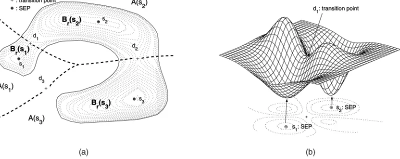
Remark.The converse of this theorem is not generally true. See Fig. 1a. In this figure, two adjacent SEPs,s1 ands3, are in the same cluster of a level setLfðrÞ, but their transition point,d3, has a valuefðd3Þgreater thanr.

4.2 A Simplified Graph for Cluster Identification

The concepts of adjacent SEPs and transition points enable us to build a weighted graph Gr¼ ðV ; EÞ, describing the connections between the SEPs, with the following elements:

1. The verticesV ofGrare SEPss1;. . .;spof (5) withfðsiÞ< r, i¼1;. . .; p.

2. The edgeEofGris defined as follows;hsi;sji 2Ewith the edge weight,!hsi;sji ¼fðdiÞ, if there is a transition point di betweensi andsjwithfðdiÞ< r. (Note that the edge weightsfðdiÞalways take positive values from (3).) The constructed graphGr¼ ðV ; EÞsimplifies the cluster structures of the level setLfðrÞand gives us an insight into the topological structures of the clusters. The next theorem, one of the main results of this paper, establishes the equivalence of the topological structures between the graph Gr and the cluster of LfðrÞ. (See Fig. 2b.)

Theorem 3.Each connected component of the graphGrcorresponds to

the cluster of the level setLfðrÞ. That is,siandsjare in the same

connected component of the graphGrif and only ifsiandsjare in the

same cluster of the level setLfðrÞ.

Proof (“only if” part). Let si and sj be in the same connected component of the graphGr. Then, there is a sequence

si¼si₀;si₁;. . .;si_h1;sih¼sj

such that sik1;sik2E for eachk¼1;. . .; j. Since sik1;sik 2E

implies that there is a transition pointdkbetweensik1 andsik

with fðdkÞ< r by the construction of the graph Gr, by Theorem 2, sik1 and sik are in the same cluster of LfðrÞ for

eachk¼1;. . .; j. Therefore, the sequence si0;si1;. . .;sih are in

the same cluster and, in particular,si andsjare in the same cluster ofLfðrÞ.

(“if” part). Let si andsj be in the same cluster, sayCi, of LfðrÞ. By Theorem 2, there is a sequence

si¼si0;si1;. . .;sih1;sih¼sj

1. An unstable manifold of an equilibrium point x is defined as

Wu_{ðxÞ ¼ fxð0Þ 2 <}n_{: lim}

t!1xðtÞ ¼xg.

such that Brðsik1Þ [BrðsikÞis connected for each k¼1;. . .; j.

We will prove that sik1;sik2E for eachk¼1;. . .; jby using

contradiction. Suppose that sik1;sik62E for some k¼1;. . .; j.

Then, by Theorem 2, the transition pointdik betweensik1 and

sikshould havefðdikÞ> r, which implies thatBrðsik1Þ [BrðsikÞ

is not connected. This is a contradiction. Therefore,sik1;sik2E

for eachk¼1;. . .; jand, so,siandsjare in the same connected

component of the graphGr. tu

This theorem implies that we can differentiate between the SEPs that belong to different clusters by constructing the weighted graphGr.

5

C

As is shown in the previous section, the weighted graph Gr¼ ðV ; EÞ plays an important role in understanding the cluster structure in a simple and implementable way. In this section, utilizing the results developed so far, we suggest a strategy to implement the graph Gr from a given data set and give an illustrative example to show how the data set can be clustered with this strategy. First, we propose the following conceptual algorithm to construct a graphGrfrom a given data set.

Algorithm 1.Constructing the GraphGr Given a data setD¼ fxk¼ ðx1k;. . .; xnkÞ

T

gNk¼1 (or its reduced dimensional representations via a linear PCA, for example);

A.O.//Initialization//

Construct a trained kernel support functionfgiven in (3). Set ai_¼min

kxikandbi¼maxkxik,i¼1;. . .; n.

A.1.//Constructing the verticesV and decomposing data points into

several disjoint sets //

M¼0; V ¼ ;; // a set of stable equilibrium points; foreach data pointxk2D,k¼1;. . .; N,do

numerically integrate (5) starting fromxkuntil it reaches an SEP, say,x_k

ifx_k2=V // makehsMþ1i

thensMþ1 xk;eV fsMþ1g [V;xk2 hsMþ1iand

M Mþ1;

elsefindsi2V such thatx_k¼si andxk2 hsii; end

A.2.//Finding the equilibrium points of system (5)//

1) Divide the region withai_xi_bi_{,i¼1;. . .; ninto several} hypercubes. The length forithedge of the hypercube is ðbi_ai_{Þ=t, wheretis the user-defined step length. Therefore,} the total number of hypercubes istd_.

2) Randomize the order of data points and initialize visitðUiÞ ¼F alsefor each hypercubeUi.

foreach data pointxk2D,k¼1;. . .; N,do find the hypercubeUi to enclosexk; ifvisitðUiÞ ¼F alse

thenfind the solution ofrfðxÞ ¼0starting fromxk; visitðUiÞ ¼T rue;

end

A.3.//Constructing the edgesE//

Identify the index-one saddle pointsdi, withfðdiÞ< r,i¼1;. . .; q, from the equilibrium points obtained in (A.2) by checking the eigenvalues of the Hessianr2_fðdiÞ.

fori¼1toqdo

1) Find a unit length eigenvectorvicorresponding to a negative eigenvalue ofr2_{fðdiÞ. Setx}þ

i ¼diþviandxi ¼divifor some small >0.

2) Numerically integrate (5) starting fromxþ_i andx

i until they approach the SEPs, saysþ_i ands

i, respectively. Sethsþi;sii 2E. end

To determine the connected components of the constructed graphGrand to assign the cluster label to each data point, we next suggest the following method, which makes repeated calls to the well-known depth-first search algorithm:

Algorithm 2.Labeling.

Given a graphGr¼ ðV ; EÞ; setindex¼0;

foreach vertexsi2V //Determining the connected components

ofGr//

visitðsiÞ ¼F alse;labelðsiÞ ¼index; end

foreach vertexsi2V ifvisitðsiÞ ¼F alse

thenindex¼indexþ1;callDF Sðsi; indexÞ; end

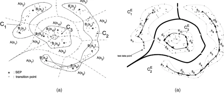
Fig. 2. (a) There are three clusters,C1,C2,C3(the regions whose boundaries are represented by solid lines) and each cluster consists of its constituent basin level cells, e.g.Bðs1Þ [Bðs2Þ. (b) Clustering by Algorithm 2. The SEPssi, denoted by, represent 10 vertices of the cunstructed weighted graphGr. The solid lines with arrows represent the unstable manifolds of the transition pointsdi, implying the eight edges ofGrthat connects two adjacent SEPs. The graphGrdetermines three extended clustered groups,CE

1,CE2,C3E, whose boundaries are represented by solid lines. A test data point, denoted by “o,” for example, converges to an SEP,s12C1E, implying that the point belongs toCE

subprocedureDF Sðsi; indexÞ //Depth-first search algorithm// begin

1)visitðsiÞ ¼T rue;labelðsiÞ ¼index; 2)foreach vertexsjsuch thathsi;sji 2E

ifvisitðsjÞ ¼F alse, thencallDF Sðsj; indexÞ; end

end

foreach SEPsi2V,i¼1;. . .; M,do //Labeling labelðxkÞ ¼labelðsiÞfor allxk2 hsiiobtained in (A.1); end

To illustrate the proposed algorithms, see Fig. 2. In this example, applying Algorithm 1, we obtain 10 SEPs,si, vertices ofGr, and eight transition points,di, where the unstable manifolds of thedi that connect two adjacent SEPs represent eight edges of Gr, as shown in Fig. 2b. Algorithm 2 is then applied to this constructed graph and we get the three connected components of Gr by identifying the cluster labels of si, thereby assigning the cluster label of each sample data point.

Remark. Computation of transition points is very crucial in constructing a graph whose topological structure is equivalent to that of the clusters described by a trained kernel support function, as in Theorem 3. Moreover, it helps us to correctly assign a cluster label to each SEP from the vertices consisting of only SEPs. To illustrate this, consider a widely used complete graph (CG) labeling strategy [1], [7], [11] applied to a restricted set of the SEPs fskgM

k¼1. The CG strategy builds an adjacency matrixAijbetween pairs ofskandsl:Aij¼1, iffðyÞ rfor all the points y on the line segment connecting sk and sl and Aij¼0, otherwise. This strategy does not work correctly for the example in Fig. 2a. In this example, the SEP,s7, is assigned to a different cluster from a group of fsig6i¼3, since, for each

i¼3;. . .;6,fðs7þðsis7ÞÞ 6rfor some2 ½0;1.

6

E

R

To demonstrate the performance of the proposed method empirically, we have conducted simulations on some clustering problems: 2D-P100, 2D-P400, and 2D-P1000 are data sets obtained from [1], [6] and 2D-N400, 2D-N800, and 2D-N1000 are data sets artificially generated from the same multimodal distribution with different sizes to compare the time complexity of the various methods. twocircles andthreecirclesjoined are well-known clustering data sets from [14] and iris,

waveform, satimage andshuttle are widely used classifica-tion data sets from the UCI repository [15].

The proposed method (Proposed) is compared with five different SVC methods; Complete Graph (CG) [1], Delaunay Diagram (DD) [11], Minimum Spanning Tree (MST), K-Nearest Neighbors (K-NN), and Reduced Complete Graph (R-CG) [6] algorithms. Here, R-CG differs from the proposed method in that it applies the CG algorithm to assign the cluster labels of the SEPs. The criteria for comparison are the cluster labeling error rate and the average CPU time of cluster labeling. Here, the labeling error rate means the percentage of the mislabeled data with respect to the clusters determined by the trained kernel support function (TKSF) of SVC in (3). This measure evaluates how accurately a chosen labeling method discriminates a connected component (cluster) from the other separate components (cluster) determined by the TKSF.2 The parameter valuesðC; qÞ can be controlled by cross validation to have a reasonable clustering result (e.g., low misclassification error rate for an a priori known, labeled data set). In our simulation, to focus on the comparison of cluster labeling error rates, we have chosenðC; qÞvalues by fixingC¼1(not using soft margins) and choosing an appropriate widthqfor each data set and then used the same values to compare the labeling performance of the different SVC methods.

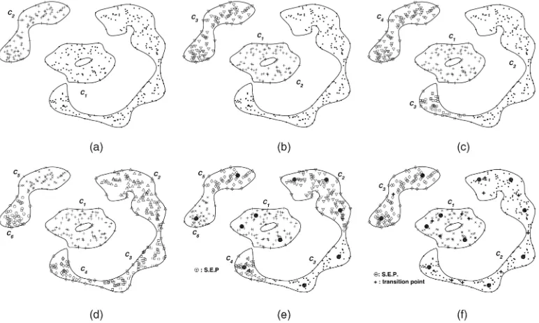
Experimental results are shown in Table 1 and Fig. 3. As is shown in Table 1, cluster labeling task is more computationally intensive than the SVC training task (QP time) and is frequently error prone. In a cluster labeling task, CG shows a relatively good labeling accuracy, but it has a heavy computational burden, and does not correctly work for some problems as in Fig. 3a. DD shows a relatively good labeling accuracy with moderate time complexity, but is very impractical for high dimensional data sets. MST and KNN show poorer labeling performance than other methods. R-CG shows a fast computing time with moderate labeling error rates, but fails frequently for a data set with highly curved cluster boundaries as in 2D-N400. On large-scale real data sets (satimage, shuttle), the cluster labeling results of only the R-CG and the proposed method are available, whereas those of other methods are not available due to their heavy time complexity and requirements of large memory. As a result, the proposed

2. The cluster labeling error rates reported in Table 1 are conceptually different from misclassification error rates for classification problems. For example, if two points within the same connected component are labeled as the same cluster by the TKSF, the labeling error has a zero value in our measure, but the misclassification error can have a nonzero value if these points have different class labels.

TABLE 1 The Experimental Results

method shows the overall best labeling accuracy with relatively good time complexity.

In summary, the proposed method has several nice features: First, it is more robust and effective in cluster labeling by checking the function values of the transition points instead of checking the function values of whole line segments as other methods (see Figs. 3 and 2a) do. Second, it focuses on the SEPs and transition points between components rather than the SVs after an SVC training step. Finally, it is inductive, i.e., it can easily assign a cluster label to unseen test data just by checking the cluster label of its corresponding SEP, whereas other methods have to retrain the data set, including a new data point to assign a cluster label to the added data point.

7

C

In this paper, we have introduced the concept of a basin level cell and developed a topological characterization of the clusters described by the SVC. We have shown that each cluster can be decomposed into its constituent basin level cells and can be extended to an enlarged clustered domain, thereby partitioning the whole data space into separate clustered domains for inductive clustering. We have also constructed a weighted graph that simplifies the topological structure of the clusters by introducing the concept of a transition point and an adjacency and established an equivalence of the topological structure between the con-structed graph. To illustrate the developed theoretical results, a clustering algorithm employing the constructed graph was given and showed, through simulation, a significant improvement in the accuracy and in the scope of cluster labeling over other SVC methods.

Until now, the analysis of the cluster structures described by the support vector clustering methods had been poorly made. We expect that our topological and dynamical characterization will pave the way for many new extensions to the support vector clustering methods.

A

This work was supported by the Korea Science and Engineering Foundation (KOSEF) under grant number R01-2005-000-10746-0.

R

[1] A. Ben-Hur, D. Horn, H.T. Siegelmann, and V. Vapnik, “Support Vector Clustering,”J. Machine Learning Research,vol. 2, pp. 125-137, 2001.

[2] C.J. Burges, “A Tutorial on Support Vector Machines for Pattern Recognition,”Data Mining and Knowledge Discovery,vol. 2, no. 2, pp. 121-167, 1998.

[3] F. Camastra and A. Verri, “A Novel Kernel Method for Clustering,”IEEE Trans. Pattern Analysis and Machine Intelligence,vol. 27, no. 3, pp. 461-464, Mar. 2005.

[4] H.K. Khalil,Nonlinear Systems.New York: Macmillan, 1992.

[5] J. Lee and H.-D. Chiang, “A Dynamical Trajectory-Based Methodology for Systematically Computing Multiple Optimal Solutions of General Non-linear Programming Problems,” IEEE Trans. Automatic Control,vol. 49, no. 6, pp. 888-899, June 2004.

[6] J. Lee and D. Lee, “An Improved Cluster Labeling Method for Support Vector Clustering,”IEEE Trans. Pattern Analysis and Machine Intelligence,

vol. 27, no. 3, pp. 461-464, Mar. 2005.

[7] B. Scholkopf, J. Platt, J. Shawe-Taylor, A.J. Smola, and R.C. Williamson, “Estimating the Support of a High-Dimensional Distribution,” Neural Computation,vol. 13, no. 7, pp. 1443-1472, 2001.

[8] D.M.J. Tax and R.P.W. Duin, “Support Vector Domain Description,”Pattern Recognition Letters,vol. 20, pp. 1191-1199, 1999.

[9] V.N. Vapnik, “An Overviewof Statistical Learning Theory,”IEEE Trans. Neural Networks,vol. 10, pp. 988-999, Sept. 1999.

[10] J. Yang, V. Estivill-Castro, and S.K. Chalup, “Support Vector Clustering through Proximity Graph Modelling,” Proc. Ninth Int’l Conf. Neural Information Processing (ICONIP ’02),pp. 898-903, 2002.

[11] R. Jensen, D. Erdogmus, J.C. Principe, and T. Eltoft, “The Laplacian PDF Distance: A Cost Function for Clustering in a Kernel Feature Space,”

Advances in Neural Information Processing Systems (NIPS),vol. 17, pp. 625-632, Cambridge, Mass.: MIT Press, 2005.

[12] M. Girolami, “Mercer Kernel Based Clustering in Feature Space,”IEEE Trans. Neural Networks,vol. 13, no. 4, pp. 780-784, July 2002.

[13] A.Y. Ng, M.I. Jordan, and Y. Weiss, “On Spectral Clustering: Analysis and an Algorithm,”Advances in Neural Information Processing Systems (NIPS),

vol. 14, 2002.

[14] UCI Repository of Machine Learning Databases, http:www.ics.uci.edu/ ~mlearn/MLRepository.html, 2006.

.For more information on this or any other computing topic, please visit our Digital Library atwww.computer.org/publications/dlib.