OneClock to Rule Them All:
Using Time in Networked Applications
Technical Report
, January 2016
Tal Mizrahi, Yoram Moses
∗Technion — Israel Institute of Technology
Abstract—This paper introduces OneClock, a generic approach for using time in networked applications. OneClock provides two basic time-triggered primitives: the ability to schedule an operation at a remote host or device, and the ability to receive feedback about the time at which an event occurred or an operation was executed at a remote host or device. We introduce a novel prediction-based scheduling approach that uses timing information collected at runtime to accurately schedule future operations.
Our work includes an extension to the Network Configura-tion protocol (NETCONF), which enables OneClock in real-life systems. This extension has been published as an Internet Engineering Task Force (IETF) RFC, and a prototype of our NETCONF time extension is publicly available as open source.
Experimental evaluation shows that our prediction-based ap-proach allows accurate scheduling in diverse and heterogeneous environments, with various hardware capabilities and workloads. OneClock is a generic approach that can be applied to any managed device: sensors, actuators, Internet of Things (IoT) devices, routers, or toasters.
I. INTRODUCTION
A. Background
Motivation.Various distributed applications require the use of accurate time, including industrial automation systems [2], automotive networks [3], and accurate measurement [4]. Sur-prisingly, while these different applications typically use stan-dard time synchronization methods (e.g., [5]), there is no standard method forusing time, and thus each of these appli-cations uses a proprietary management protocol that invokes time-triggered operations. In this paper we present a generic approach that allows the use of accurate time to manage various diverse devices, from routers to toasters.1
Why NETCONF? A formal announcement by the Inter-net Engineering Steering Group (IESG), released in March 2014 [7], declared that the IETF is encouraging the use of NETCONF [8], rather than the Simple Network Management Protocol (SNMP) [9]. Indeed, the networking community is quickly shifting from SNMP-based Management Information Bases (MIB) to modules based on YANG [10], the modeling language used by NETCONF. During the writing of this paper, the IETF Active Internet Draft list [11] consisted of 256 drafts
This technical report is an extended version of [1], which was accepted
to IEEE/IFIP NOMS 2016.
∗Yoram Moses is the Israel Pollak academic chair at Technion.
1Paraphrasing the 25-year old gimmick of the network-managed toaster [6].
that define YANG data models [12], and only 21 drafts that define MIBs.
NETCONF and YANG are gaining momentum in the con-text of various diverse applications, not only in the traditional realm of routers and switches, but also in other applications, such as Virtualized Network Functions [13] and Internet of Things (IoT) devices [14], [15]. NETCONF is being adopted not only by the IETF, but also by other organizations, such as the Open Networking Foundation [16], and the Metro Ethernet Forum [17].
We chose to use NETCONF as a baseline for OneClock, due to its increasing adoption rate and diversity of applications and environments.
B. The OneClock Protocol
In this paper we introduce a generic protocol forusing time in networked applications. The protocol is defined as an extension of NETCONF. A full specification of this extension, including an open-source YANG module that defines the extension, has been published as an RFC [18].
Our OneClock extension defines two basic time-related primitives: (i)scheduling: a NETCONF client2 can schedule
a Remote Procedure Call (RPC) to be performed by a NET-CONF server at a prescribed future time, and (ii) reporting: a NETCONF client can receive feedback about the time of execution of an RPC, or a notification about the time of occurrence of a monitored event.
OneClock can be used in various important use cases, such as invoking scheduled operations in diverse applications, tak-ing coordinated snapshots of a system, or performtak-ing network-wide atomic commits.
C. OneClock: Accurate Scheduling
One of the greatest challenges in our approach is to accu-ratelyschedule network operations. Even if a managed device (server) keeps an accurate clock, it is difficult to guarantee that scheduled operations are performed very close to their scheduled times. The actual execution time may depend on the processing power of the server, on its operating system, and its load due to other tasks that run in parallel.
2We follow the NETCONF terminology; managed devices, referred to as servers, are managed by one or moreclient.
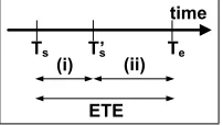
We propose a prediction-based approach that allows a client to accurately schedule network operations without prior knowledge about the servers’ performance. The approach is based on measuring the Elapsed Time of Execution (ETE) of each RPC, and using previous ETE measurements to predict the next ETE.
e
s s
Fig. 1: Elapsed Time of Execution (ETE): ETE =Te−Ts.
The ETE is defined to be Te−Ts (see Fig. 2), where Ts is the scheduled start time of the RPC, and Te is the actual completion time of the RPC. The actual start time of the RPC is denoted byT0
s. Hence, as depicted in Fig. 1, the ETE is affected by two non-deterministic factors: (i) the server’s ability to accurately start the operation, and (ii) the running time of the RPC.
For each scheduled operation (see the numbered steps in Fig. 2):3
1) The client predicts the ETE of the next RPC based on previous measurements of the scheduled time and execution time.
2) For a given desired execution time, Td, the client sched-ules the operation to be performed atTd−ET E. 3) The server reports the actual time of execution,Te, back
to the client, allowing the client to use this feedback for scheduling future operations.
server client rp
c (T
1)
rpc -re
ply
(T2 )
T1
time
scheduled time T2
measured ETE
execution time
rp c (T
s)
rpc -re
ply
(Te )
Ts scheduled time
Ts= Td- ETE Td
desired execution time
...
compute predicted ETE
based on ETE measurements 1
2 3
Teexecution timeactual
Fig. 2: Prediction-based scheduling: by predicting the ETE, a client can control when the RPC will be completed.
Notably, our scheduling approach allows a NETCONF client to accurately schedule network operations in a hetero-geneous environment, where the performance of the managed servers is not necessarily known in advance.
D. Related Work
The use of the time-of-day in network management is a common practice. Time-of-day routing [19] routes traffic to different destinations based on the time-of-day. Scheduled
3We follow the notation of [8], where Remote Procedure Calls are denoted
by uppercase RPC, and the messages that carry RPCs are denoted by lowercaserpc.
operations [20], [21] allow various policies and configurations to be applied at specific time ranges. The work of [22] analyzed the use of timed path updates in Software Defined Networks. This paper introduces a more general framework that allows time-triggered operations in any network managed device, and enables accurate scheduling of network operations in a heterogeneous environment. The work of [23] suggested a method for accurate scheduling in switches and routers using Ternary Content Addressable Memories (TCAM). Our scheduling scheme is more generic, as it makes no assumption about the hardware of the managed devices.
The literature is rich with works that analyze and predict program running times, e.g., [24]–[28]. In this paper we use time series analysisto predict the execution time of aremote operation, allowing to perform accurate scheduling of the requested operation.
E. Contributions
The main contributions of this paper are:
• We introduce OneClock, a generic approach for using time in networked applications. OneClock defines two basic primitives,schedule, andreport. Several use cases that demonstrate the merits of OneClock are presented.
• We present a scheduling approach that allows accurate scheduling by predicting the server’s execution time. We analyze three prediction algorithms: two average-based algorithms, and a Kalman-Filter-based algorithm.
• We define a OneClock extension to NETCONF, which has been published as an IETF RFC.
• We have implemented a prototype of the NETCONF
time extension. Our prototype is available as open source. Our experimental evaluation demonstrates how accurately events can be scheduled over a network.
II. USINGONECLOCK INPRACTICE
In this section we describe three use cases that illustrate how the two time-triggered primitives, scheduling and reporting, can be used in distributed systems.
A. Coordinated Operation
It is often desirable to coordinate a set of events or oper-ations that should take place at different nodes in the system at the same time,4 or should occur according to a specific
order. The schedule primitive can be used to coordinate events occurring in actuators in a factory product line [2], to coordinate a routing change in a network [29], or to orchestrate events in scientific experiments [30].
Using OneClock, a client canschedulea simultaneous event at multiple servers, or define a sequence of scheduled times that determine the order and relative timing of events.
4In practical systems it is typically not possible to coordinate events to
s
s scheduled time
(a) Scheduled RPC.
e
e RPC executed
(b) Reporting the execution time.
s e
e s
RPC executed
(c) Reporting the execution time of a scheduled RPC.
s
s no
tifi ca
tio n
scheduled time
(d) Scheduled RPC with notification.
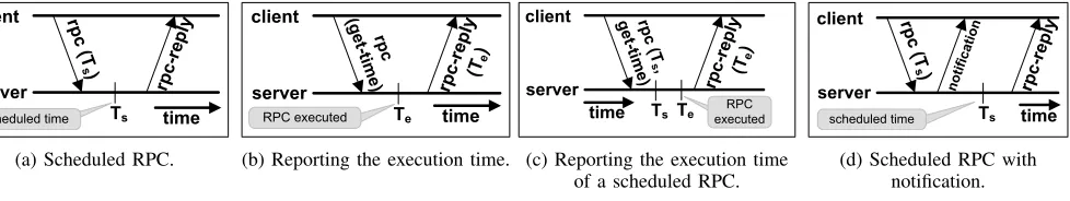
Fig. 4: The time capability in NETCONF.
Client
Server 1 Server 2 Server n
T T T
(a) Coordinated operations: all servers perform the operation at the same time,T.
Client
Server 1 Server 2 Server n
T T T
(b) Coordinated snapshot: all servers send their state to the
client at the same time.
Fig. 3: Coordinated operations and coordinated snapshots.
B. Coordinated Snapshot
In many applications it is desirable to monitor events or statistics with respect to a common time reference.
A client can perform a coordinated snapshot, i.e., capture the state of a monitored attribute at all the servers at the same time. While a simultaneous snapshot does not produce a consistent distributed snapshot [31], it provides a coordinated snapshot of the servers’ state. For example, when collecting statistics from all the servers, it is most useful to capture the information at the same time in all servers. In power grid networks [32], synchrophasor measurements are used for monitoring the operation of a power grid. These measurements must be synchronized, so as to allow correct system-wide processing.
OneClock enables coordinated snapshots; using the sched-ule primitive, a client can schedule a NETCONF get-config operation [8] to be taken at time T, causing all the servers to send their response at the same time (Fig. 3b).
C. Network-wide Atomic Commit
The NETCONF commit [8] is an RPC that commits the candidate configuration, i.e., copies the candidate configu-ration to the running configuration. This operation allows the client to prepare a set of configuration updates in the candidate datastore, and then apply them at once with the commit operation.
It is often desirable to perform a network-wide atomic commit, where either all the servers successfully perform the commit operation, or if some of the servers are not able to perform the commit, then none of the servers perform it.
Atomic commits can be performed using NETCONF with-out our time extension, but potentially at the cost of a tem-porary state of inconsistency, where different servers use
dif-ferent configuration versions (Fig. 5). This can be done using the NETCONF confirmed commit procedure. This procedure requires two steps: (i) the client sends a first commit message to all the servers, causing them to switch to the candidate configuration, and (ii) the client sends a confirming commit message to all the servers, finalizing the commit procedure. If the two phases are not completed successfully, or if the client cancels the commit, the servers roll back to the previous configuration.
The OneClock schedule primitive enables a clean and straightforward approach to network-wide commits, as illus-trated in Fig. 5. The client sends a scheduled commit message to the servers, to be performed at a future timeT. If some of the servers fail to schedule the commit operation, the client can cancel the commit before time T, leaving all the servers at the current configuration.
III. NETCONF TIMEEXTENSION
We introduce an extension to the NETCONF protocol that allows time-triggered operations. The extension is defined as a new capability[8]. Details are presented in [18].
A. Overview
The time capability provides two main functions:
• Scheduling. When a client sends an rpc message to a server, the message may include thescheduled-time
parameter, denoted byTsin Fig. 4a. The server then starts to execute the RPC as close as possible to the scheduled timeTs, and once completed the server can respond with anrpc-replymessage.
• Reporting. When a client sends an rpc message to a server, the message may include a get-time element (see Fig. 4b), requesting the server to return the execution time of the RPC. In this case, after the server performs the RPC it responds with an rpc-reply that includes the
execution-timeparameter, specifying the timeTeat which the RPC was completed.
server A
Time client co
m m
it
ca nc
el
OK
server B
err or
OK
Old configuration
New configuration
co m
m it (T
)
ca n
ce l
OK erro
r
OK
c om
m it (T
)
T
server A client
server B
(a) (b)
co m
m it
Fig. 5: Atomic commit: (a) NETCONF confirmed commit, without using time. (b) Time-triggered commit.
slightly different time than Ts, for example if the server is tied up with other tasks at time Ts.
The report abstraction, presented in Sec. I-B, allows the client to receive information about the execution time of an RPC, or to receive notifications about the time of occur-rence of events. The former can be implemented using the
get-time procedure we defined, while the latter is already supported in NETCONF by using notifications that include the
eventTimeparameter [33].
B. Applying the Time Primitives to Various Applications
The time capability specification we defined [18] includes a YANG module that adds the two new primitives,scheduleand report, as two parameters in all the RPC types defined in [8]. For example, this YANG module enables scheduledcommit, and scheduledset-configRPCs.
Notably, the time primitives are not limited to the RPCs defined in [8]. If a new YANG module defines a new RPC, the module can include the time parameters, allowing the new RPC to use the time primitives. Our open source code includes two such examples:
• We enhanced the well-knowntoasterYANG module [34], by allowing the make-toastoperation to be a sched-uled RPC.
• We created a new YANG module called test, which
triggers the server to perform a configurable command line. Using the scheduleparameter, the testRPC can be used as a remote variant of the well-known Cron [35] command in Linux.
The report primitive can be used not only by applying the get-time parameter, but also by other means that are inherently possible when using NETCONF. The time of occurrence of important events can be sent to the client using a NETCONF notification [33], or can be included in the NETCONF data model. For example, the YANG data model that defines a log entry may include the time-of-day in each log entry.
C. Notifications and Cancellation Messages
1. Notifications
As illustrated in Fig. 4a, after a scheduled RPC is executed the server sends an rpc-reply. The rpc-reply may
arrive a long period of time after the rpc message was sent by the client, leaving the client without a clear indication of whether the rpc was received. Therefore, we define an optional netconf-scheduled-message notification (Fig. 4d), which provides an immediate acknowledgment of the scheduled RPC. As illustrated in Fig. 4d, when the server receives a scheduled RPC it sends a notification that includes themessage-idof the scheduled RPC.
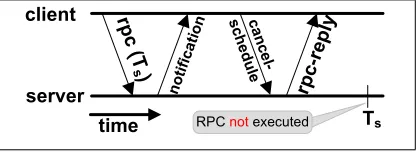
2. Cancellation Messages
A client can cancel a scheduled RPC by sending a cancel-schedule RPC (Fig. 6). The
cancel-schedule RPC, defined in this document,
can be used to enforce the coordinated network-wide commit described in Sec. II-C.
server
client rp
c (T
s)
rpc -re
ply
Ts no
tifi ca
tio n ca
nc e l-sc
h ed
u le
time RPC not executed
Fig. 6: Cancellation message.
D. Clock Synchronization
The time capability we defined requires clients and servers to maintain clocks. It is assumed that clocks are synchronized by a clock synchronization method, e.g., [5], [36].
E. Acceptable Scheduling Range
A server that receives a message that is scheduled to be performed at timeTs verifies that the valueTs is not too far in the past or in the future. As illustrated in Fig. 7, the server verifies that Ts is within the acceptable scheduling range.
IfTsoccurs in the past and within the acceptable scheduling range, the server performs the RPC as soon as possible
The scheduling bound defined by sched-max-future
from server failures, or from multiple clients trying to schedule conflicting operations.
IV. PREDICTION-BASEDSCHEDULING
Our scheduling approach is based on using previous mea-surements of the Elapsed Time of Execution (ETE).
Based on the ETE measurements, the client uses the pre-diction approach illustrated in Fig. 8. The prepre-diction approach consists of three steps:
1) When a scheduled operation is required to take place at time Td, the client uses previous ETE measurements, x[1], . . . , x[n−1], to predict the next ETE, denoted by s[n|n−1].
2) The next scheduled time is Ts=Td−s[n|n−1]. 3) The client updates its measurement set based on the
feedback received from the server about the execution timeTe.
In the rest of this section we describe the two main com-ponents of our scheduling approach, the ETE measurements, and the ETE prediction.
A. ETE Measurements
We analyze two measurement methods:
Periodic probing. This approach uses ETE measurements that are taken periodically at a constant frequency. In systems that require periodic operations, these ETE measurements are inherently available. In other systems, the client can proac-tively send periodic scheduled RPCs to every server in order to probe the ETE. The main drawback of periodic probing is that it can potentially consume unnecessary resources, both at the client and at the server.
Burst probing. The second approach uses an on-demand burst of probe RPCs; when a scheduled RPC is required, the client initiates a burst of N scheduled RPCs, performed at
Time Ts
Server receives scheduled RPC.
acceptable scheduling range sched-max-past sched-max-future
Fig. 7: Acceptable scheduling range: defined by two config-urable parameters: sched-max-future and sched-max-past.
measured T
e
x[n] = T
e- T s
ETE measurements x[1], x[2], , x[n-1]
ETE Prediction: s[n|n-1]
Scheduling:
Ts= Td- s[n|n-1] 1
2 3
Fig. 8: Prediction-based scheduling approach.
a fixed frequency. This approach does not require resource consumption in the absence of actual scheduled RPC requests, but the prediction is potentially less accurate, since it is based on a smaller number of measurements.
Note that both approaches require the probe RPCs to be similar in terms of performance and running time to the future RPC for which the prediction is required.
B. ETE Prediction Algorithms
We analyzed three prediction algorithms, Average, FT-Average, andKalman. We now describe these algorithms.
1. Baseline
The baseline for comparison in our evaluation is the simplest approach which assumess[n] = 0, and therefore assignsTs= Td. In this approach the prediction error is equal to the ETE.
2. Average Algorithm
The Average algorithm performs an average of the lastN measurements:
s[n|n−1] = 1
N N
X
j=1
x[n−j] (1)
3. Fault-tolerant Average (FT-Average) Algorithm
The Fault-tolerant Average [37] performs an average of the last N measurement samples, after ignoring the highest and the lowest measurement values. Hence, this approach masks the most noisy or erroneous measurement of theN samples.
s[n|n−1] =
1
N N
P
j=1
x[n−j], ifN <3
1
N−2(
N
P
j=1
x[n−j]
− max
1≤j≤Nx[n−j]
− min
1≤j≤Nx[n−j]), otherwise (2)
4. Kalman Filtering Algorithm
Kalman Filtering [38] is one of the most well-known data fusion and estimation methods. One of its significant advantages is that it is the optimal estimator in systems with white Gaussian noise.
The algorithm we use is a one-dimensional Kalman Filter. Our terminology and notations are based on the standard literature, e.g., [39].
x[n] The observed ETE of thenthsample.
s[n] The estimated ETE atn, given the measurements up ton.
s[n|n−1] The estimated ETE atn, given the measurements up ton−1.
w[n] The ETE signal noise of thenthsample. v[n] The measurement noise of thenthsample.
P[n] The estimated variance of the ETE.
P[n|n−1] The estimated variance atn, given the measurements up ton−1.
K[n] The Kalman gain.
W[n] The estimated variance ofw[n], given the measure-ments up ton−1.
V[n] The estimated variance ofv[n], given the measure-ments up ton−1.
TABLE I: Kalman Filter Notations
transition coefficient is 1. Hence, the Kalman system equation is given by 3.
s[n] =s[n−1] +w[n] (3)
The Kalman observation equation is given by:
x[n] =s[n] +v[n] (4)
Based on the two equations above, we present the prediction equations and the update equations, which are the core of the Kalman Filtering algorithm.
Prediction equations.The client uses the prediction equa-tions in step 1 of Fig. 8 to estimate the next ETE based on the firstn−1measurements.
s[n|n−1] =s[n−1] (5)
P[n|n−1] =P[n−1] +W[n] (6)
Update Equations. The client uses the update equations in step 3 of Fig. 8 to update its state based on the new measurement, x[n].
s[n] =s[n|n−1] +K[n](x[n]−s[n|n−1]) (7)
K[n] = P[n|n−1]
P[n|n−1] +V[n] (8)
P[n] = (1−K[n])P[n|n−1] (9)
Variance estimation. W[n] is defined to be the estimated variance of w[n], andV[n]is the estimated variance ofv[n]. By Eq. 3 and Eq. 4, we have w[n] = s[n]−s[n−1], and v[n] =x[n]−s[n]. Hence, the variance of w[n]andv[n]can
be estimated by thesample variance using the last N values of x[·] ands[·], as follows:
W[n] = 1
N · N
X
i=1
((s[n−i]−s[n−i−1])−
(1
N · N
X
j=1
(s[n−j]−s[n−j−1])))2
(10)
V[n] = 1
N · N
X
i=1
((x[n−i]−s[n−i])−
(1
N · N
X
j=1
(x[n−j]−s[n−j])))2
(11)
V. EVALUATION
A. Background
We implemented a prototype of the NETCONF time ca-pability. The prototype was implemented as an extension to the OpenYuma [40], a NETCONF software implementation written in C over Linux. Our code is publicly available as open source [41].
Goal. The goal of the experiments was to evaluate our prediction-based scheduling approach over various machines, platforms, and under various workloads.
Method. We evaluated the three prediction algorithms (Sec. IV) on Linux-based servers in two academic testbeds, Emulab [42] and DeterLab [43], and in two public cloud platforms, Microsoft Azure [44], and Amazon Web Services (AWS) [45]. Our measurements were performed on over 100 servers, for a total duration of over 5000 hours, summing up to over 3 million measurement samples.
Our results are based on measurements that were performed using a commit RPC on the well-known toaster YANG module [34]. In each experiment a NETCONF client sent scheduled RPC messages to a server, and the client recorded the Ts andTevalues. The experiments produced log files (at the client) containing Ts and Te values, and then the three prediction algorithms were run offline.5 The three algorithms
were run withN = 8in most of the runs6, except for specific
runs in which the value ofN was different, as described below. We quantify the accuracy of our prediction by observing the mean absolute prediction error. The prediction error of an RPC is defined as the difference between the predicted ETE and the measured ETE.
5In the current prototype we have not integrated the prediction algorithm
logic into the NETCONF client. The prediction algorithms were run offline on the log files of the NETCONF client.
6N is the number of measurement samples used in each prediction
0.00001 0.0001 0.001 0.01 0.1 1
Type I Type II Type III Type IV Type V Type VI
M ea n A b so lu te P re d ic ti o n E rr o r [s ec o n d s -lo g .] Server Type Baseline Average FT-Average Kalman
(a) Performance on different platforms.
0 0.002 0.004 0.006 0.008 0.01 0.012 0.014
1 10 100 1000
M e a n A b so lu te P r e d ic ti o n E r r o r [ se c o n d s]
Measurement Period [seconds] Baseline Average FT-Average Kalman
(b) Periodic measurement.
0 0.002 0.004 0.006 0.008 0.01 0.012 0.014
0 5 10 15
M ea n A b so lu te P re d ic ti o n E rr o r [s ec o n d s]
Number of Samples per Burst Baseline Average FT-Average Kalman
(c) Bursty measurement.
Fig. 9: Performance on various machine types (a). Type V machines were used in (b) and (c).
0 0.005 0.01 0.015 0.02 0.025
0 50 100 150
A b so lu te P r e d ic ti o n E r r o r [ se c o n d s] Time [seconds] 1 VM - Baseline 1 VM - FT-Average 20 VMs - Baseline 20 VMs - FT-Average
(a) Performance on shared machine with 20 VMs, compared to machines with one VM.
0 0.01 0.02 0.03 0.04 0.05
0 50 100 150
A b so lu te P r e d ic ti o n E r r o r [ se c o n d s] Time [seconds] Baseline FT-Average Stress - Baseline Stress - FT-Average
(b) Performance on stressed server compared to unstressed server.
0 0.01 0.02 0.03 0.04 0.05
0 50 100 150
A b so lu te P r e d ic ti o n E r r o r [ se c o n d s] Time [seconds] Baseline Average FT-Average Kalman
(c) Occasional error spikes during a stress experiment.
Fig. 10: Instantaneous prediction error viewed over a 150second period. The behavior shows peaks under synthetic workload. (a) was measured on Azure, and (b), (c) on Type V machines.
B. Experiment I: Performance on different platforms
In this experiment (Fig. 9a) we compared the prediction error of the three prediction algorithms on various server types. The prediction in this experiment was based on periodic sampling, with a measurement period of 8 seconds.7 The list of servers we tested is presented in Table II.
Type Description Platform / class
I Public cloud (shared tenancy), 1GB memory
Amazon / t2.micro
II Public cloud (shared tenancy), 768MB memory
Azure / A0
III Xeon E3 LP 2.4 GHz, 16GB memory
DeterLab /
MicroCloud IV Xeon 2.1 GHz, 4GB memory DeterLab / pc2133 V Quad Core Xeon E5530 2.4 GHz,
12GB memory
Emulab / d710
VI Dual Core Opteron 1.8 GHz, 4GB memory
DeterLab / bvx2200
TABLE II: Machine types.
As shown in Fig. 9a, the prediction algorithms significantly reduced the prediction error compared to the baseline ap-proach. The experiment shows that in most of the cases FT-Average produces the lowest error.
7The measurement period is the elapsed time between two consecutive
measurements.
C. Experiment II: Periodic vs. bursty measurement
We compared periodic measurement and burst-based mea-surement (see Fig. 9b and 9c). The periodic meamea-surement was performed at various measurement periods, and the burst measurement was performed with various burst sizes, and with a fixed period of one measurement per second. We note that in this experiment the error produced by the three algorithms is very similar.
Interestingly, the results show that a burst of 4 samples suffices to produce similar results to a periodic measurement. In the periodic measurement (Fig. 9b) the lowest prediction error was achieved with a period of one measurement per second. We were not able to test lower measurement periods due to a performance limitation in the NETCONF client we used.
Another interesting observation is that when the measure-ment period was on the order of one minute or more we observed slightly higher ETE values (Fig. 9b) than when the measurement period was on the order of a few seconds. This can be explained by the server’s cache policy, which allows better performance for operations that are performed frequently.
D. Experiment III: Performance under synthetic workload
NET-CONF servers. We used two methods to stress the machines: (i) We used the lookbusy [46] utility to inject synthetic workload (Fig. 10b). We configured the utility to run at a CPU utilization of 95% and at a memory utilization of 95%. (ii) We used the Azure platform to run multiple VMs on the same physical machine (Fig. 10a). We ran 20 VMs on the same machine, where one of the VMs was the NETCONF server.
During the stress experiments we observed that most of the ETE measurements were unaffected by the stress, but as depicted in Fig. 10a and 10b, there were occasional spikes in the ETE, causing temporary high prediction error. As shown in Fig. 10a and 10b, prediction error of the FT-Average algorithm during the ETE spikes is slightly lower than the baseline error, and during most of the run the prediction error of the FT-Average is significantly lower than the baseline error.
Fig. 10c compares the three prediction approaches during an ETE spike. As illustrated in Fig. 10c, the FT-Average algorithm was the most resilient to these spikes, as it ignores the maximal and minimal measurement samples, and thus ignores the peak ETE value. As depicted in the figure, the two other algorithms were more sensitive to these spikes.
VI. DISCUSSION
Prediction method.As discussed in the previous sections, we analyzed three prediction algorithms. Kalman filtering was used as it is one of the most celebrated and popular data fusion algorithms. The Average approach was chosen due to its simplicity, and FT-Average due to its resilience to occasional isolated noisy measurements.
The experimental results show that the prediction error offered by the three algorithms is similar, and is signifi-cantly lower than the baseline error. The FT-Average approach showed slightly lower prediction error in most of the experi-ments. FT-Average is especially advantageous in the presence of occasional spikes in the ETE, as it inherently ignores the erroneous measurement. Interestingly, even a short burst of N = 4measurements allows the simple FT-Average algorithm to predict the ETE with a very low prediction error.
Measurement period. The measurement period is the elapsed time between two consecutive measurements. Frequent measurements may be more sensitive to changes in the ETE, and allow a more accurate prediction. On the other hand, if measurements are performed too frequently they may affect the server’s performance. Since the client continuously moni-tors the prediction error, the client can dynamically change the measurement period for each server to improve the prediction error. Thus, an interesting extension to our work would be to implement an algorithm that dynamically changes the measurement period for each server.
RESTCONF. An interesting next step would be to extend the scope of our work, and apply it to the emerging REST-CONF [47]. This work would be especially interesting in the context of resource constrained servers, such as IoT devices.
Multiple RPC types.The ETE of an RPC depends on the RPC type. Thus, the prediction method should be used on a per-RPC-type basis. A possible extension of our work would be to consider how to predict the ETE of RPC type A using measurements of RPC type B.
Time zone issues. Since the client and servers may be spread across multiple time zones. The NETCONF date-and-time format specifies the time zone for each timestamp, thereby avoiding ambiguity in the timestamp value. Moreover, to avoid problems that may arise during Daylight Saving Time (DST) changes, the client can invoke scheduled RPCs using the UTC time zone, which is not subject to DST changes.
Impact of the network delay on the measurements.When a client sends a scheduled RPC message, the message must be sent in advance, allowing the message to arrive to the server before the scheduled time. Thus, as the network delay increases, the client must send the scheduled RPC sooner. In our experiments we considered the network delay when planning the time at which RPCs are sent. Note that the ETE is a metric of the servers’ performance, and is not affected by the network delay.
Inter-RPC influence.The ETE of an RPC may be affected by other RPCs that are running in parallel, or are scheduled to run in parallel. The prediction approach presented in this paper estimates the RPC’s execution time, given that the server is subject to workload by other tasks or other RPCs running in parallel. In our evaluation we mimicked these scenarios by synthetically creating additional workload on the servers.
VII. CONCLUSION
OneClock is a generic approach for using accurate time in distributed applications. As NETCONF is gaining momentum and penetrating various new network applications, OneClock seems like a natural extension that can add the time dimension to network configuration and management.
We analyzed three prediction algorithms, and found the simple FT-Average to be the most accurate algorithm in most of the experiments. Our experimental evaluation confirms that prediction-based scheduling provides a high degree of accu-racy in various diverse environments, decreasing the prediction error by an order of magnitude compared to the na¨ıve baseline approach.
VIII. ACKNOWLEDGMENTS
REFERENCES
[1] T. Mizrahi and Y. Moses, “OneClock to Rule Them All: Using Time in Networked Applications,” in IEEE/IFIP Network Operations and
Management Symposium (NOMS), 2016.
[2] K. Harris, “An application of IEEE 1588 to industrial automation,” in
International IEEE Symposium on Precision Clock Synchronization for
Measurement Control and Communication (ISPCS), 2008.
[3] IEEE, “Time-Sensitive Networking Task Group,” http://www.ieee802. org/1/pages/tsn.html, 2016.
[4] P. Moreira, J. Serrano, T. Wlostowski, P. Loschmidt, and G. Gaderer, “White rabbit: Sub-nanosecond timing distribution over ethernet,” in
International IEEE Symposium on Precision Clock Synchronization for
Measurement Control and Communication (ISPCS), 2009.
[5] IEEE TC 9, “1588 IEEE Standard for a Precision Clock Synchronization Protocol for Networked Measurement and Control Systems Version 2,”
IEEE, 2008.
[6] “The Internet Toaster,” http://www.livinginternet.com/i/ia myths toast. htm.
[7] “Writable MIB Module IESG Statement,” https://www.ietf.org/iesg/ statement/writable-mib-module.html, 2014.
[8] R. Enns, M. Bjorklund, J. Schoenwaelder, and A. Bierman, “Network configuration protocol (NETCONF),” IETF, RFC 6241, 2011. [9] J. Case, M. Fedor, M. Schoffstall, and C. Davin, “A simple network
management protocol (SNMP),” IETF, RFC 1157, 1990.
[10] M. Bjorklund, “YANG - A Data Modeling Language for the Network Configuration Protocol (NETCONF),” IETF, RFC 6020, 2010. [11] “Active Internet-Drafts,” https://datatracker.ietf.org/doc/active/, 2015. [12] B. Claise, “YANG data models statistics,” http://www.claise.be/
YANGPageMain.html, 2015.
[13] R. Penno, P. Quinn, D. Zhou, and J. Li, “YANG Data Model for Service Function Chaining,” IETF, draft-penno-sfc-yang-13, work in progress, 2015.
[14] A. Sehgal, V. Perelman, S. Kuryla, and J. Sch¨onw¨alder, “Management of resource constrained devices in the internet of things,”Communications
Magazine, IEEE, vol. 50, no. 12, pp. 144–149, 2012.
[15] J. Sch¨onw¨alder and A. Sehgal, “Management of the Internet of Things,” http://cnds.eecs.jacobs-university.de/slides/2013-im-iot-management. pdf, 2013.
[16] Open Networking Foundation, “OpenFlow Management and Configura-tion Protocol (OF-Config 1.2),” 2014.
[17] Metro Ethernet Forum, “Service OAM Fault Management YANG Mod-ules,”MEF 38, 2012.
[18] T. Mizrahi and Y. Moses, “Time Capability in NETCONF,” IETF, RFC 7758, 2016.
[19] G. R. Ash, “Use of a trunk status map for real-time DNHR,” in
International TeleTraffic Congress (ITC-11), 1985.
[20] D. Levi and J. Schoenwaelder, “Definitions of managed objects for scheduling management operations,” IETF, RFC 3231, 2002. [21] K. Watsen, “Conditional Enablement of Configuration Nodes,” IETF,
draft-kwatsen-conditional-enablement, work in progress, 2013. [22] T. Mizrahi, E. Saat, and Y. Moses, “Timed consistent network updates,”
inACM SIGCOMM Symposium on SDN Research (SOSR), 2015.
[23] T. Mizrahi, O. Rottenstreich, and Y. Moses, “TimeFlip: Scheduling network updates with timestamp-based TCAM ranges,” inIEEE
IN-FOCOM, 2015.
[24] M. A. Iverson, F. ¨Ozg¨uner, and L. C. Potter, “Statistical prediction of task execution times through analytic benchmarking for scheduling in a heterogeneous environment,”IEEE Trans. Computers, vol. 48, no. 12, pp. 1374–1379, 1999.
[25] E. Ipek, B. R. de Supinski, M. Schulz, and S. A. McKee, “An approach to performance prediction for parallel applications,” inEuro-Par, 2005. [26] P. Giusto, G. Martin, and E. A. Harcourt, “Reliable estimation of execu-tion time of embedded software,” inConference on Design, Automation
and Test in Europe (DATE), 2001.
[27] M. A. Iverson, F. ¨Ozg¨uner, and G. J. Follen, “Run-time statistical estima-tion of task execuestima-tion times for heterogeneous distributed computing,” in
International Symposium on High Performance Distributed Computing
(HPDC), 1996.
[28] G. Bontempi and W. Kruijtzer, “A data analysis method for software performance prediction,” inConference on Design, Automation and Test
in Europe (DATE), 2002.
[29] S. Hares and M. Chen, “Summary of I2RS Use Case Requirements,” IETF, draft-ietf-i2rs-usecase-reqs-summary-01, work in progress, 2015.
[30] M. Lipinski, “White Rabbit - Ethernet-based solution for sub-ns synchronization and deterministic, reliable data delivery,” http://maciejlipinski.pl/myPage/docs/presentations/WR IEEE802-Tutorial-Geneve2013.pdf, 2013.
[31] K. M. Chandy and L. Lamport, “Distributed snapshots: Determining global states of distributed systems,”ACM Trans. Comput. Syst., vol. 3, no. 1, pp. 63–75, 1985.
[32] B. Dickerson, “Time in the power industry: how and why we use it,” Arbiter Systems, technical report, http://www.arbiter.com/ftp/datasheets/ TimeInThePowerIndustry.pdf, 2010.
[33] S. Chisholm and H. Trevino, “NETCONF Event Notifications,” IETF, RFC 5277, 2008.
[34] Toaster YANG Module, http://www.netconfcentral.org/modulereport/ toaster, 2015.
[35] “Cron - Linux man page,” http://linux.die.net/man/8/cron, 2015. [36] D. Mills, J. Martin, J. Burbank, and W. Kasch, “Network time protocol
version 4: Protocol and algorithms specification,” IETF, RFC 5905, 2010.
[37] J. Lundelius and N. A. Lynch, “A new fault-tolerant algorithm for clock synchronization,” inSymposium on Principles of Distributed Computing
(PODC), 1984.
[38] R. E. Kalman, “A new approach to linear filtering and prediction problems,” Journal of Fluids Engineering, vol. 82, no. 1, pp. 35–45, 1960.
[39] A. Papoulis and S. U. Pillai,Probability, random variables, and
stochas-tic processes. Tata McGraw-Hill Education, 2002.
[40] OpenYuma, https://github.com/OpenClovis/OpenYuma, 2015. [41] “OneClock source code,” https://github.com/TimedSDN/Yuma-Time,
2015.
[42] Emulab — Network Emulation Testbed, http://www.emulab.net, 2015. [43] The DeterLab project, http://deter-project.org/about deterlab, 2015. [44] Microsoft Azure, https://azure.microsoft.com, 2015.
[45] Amazon Web Services, http://aws.amazon.com, 2015.
[46] D. Carraway, “lookbusy — a synthetic load generator,” https://www. devin.com/lookbusy, 2015.