Developing a Model of Heterogeneity in Driver’s Behavior

(1)

183 International Journal of Transportation Engineering, Vol. 5/ No. 2/ Autumn 2017

Developing a Model of Heterogeneity in Driver’s Behavior

Mohammad Hossein Noranian1, Ahmad Reza Tahsiri2

Received: 08. 01. 2017 Accepted: 30. 05. 2017

Abstract

Intelligent Driver Model (IDM) is a well-known microscopic model of traffic flow within the traffic engineering societies. While it is a powerful technique for modeling traffic flows, the Intelligent Driver Model lacks the potential of accommodating the notion of drivers’ heterogeneous behavior whenever they are on roads. Concerning the above mentioned, this paper takes the lane to recognize the heterogeneity in drivers’ behavior based on Heterogeneity Vector. Heterogeneity vector is an integral part of a new model that holds the potential to provide a method that in turn can accommodate the effect of the above mentioned differentiation in the traffic pattern. The Intelligent Driver Model in combination to Heterogeneous vector results to Intelligent Driver Model Heterogeneous Calibration (IDMHC) which in turn has the capability to improve the accuracy of IDM calibration, and as a result, enhances its performance under real conditions of traffic systems. Following the pre-stated, the study formulates that, the heterogeneity vector, as an output of the computation block, will apply in the simulation of the traffic of vehicles. To validate the performance of the IDMHC model, NGSIM project has been applied. As such, the most notable contributions of this study are, presenting a new method for calibration of microscopic flow model based on individual trajectory data, depicting the differences among drivers based on the newly defined heterogeneity measure, and illustrating the differences among drivers shape, traffic patterns that are causing different distributions of macroscopic variables such as travel time. Based on the study, the results obtained depicts that the difference between the presumed values regarding the IDM parameters has a great difference when compared with the calculated values for each vehicle based on a 50% variance. These results have the likelihood to significantly affect the mode in which microscopic models simulate and predict the traffic situation.

Keywords: Microscopic modeling, heterogeneity, driver behavior, intelligent driver model (IDM), traffic simulation

Corresponding author E-mail: [email protected]

1_{PhD Candidate, Systems and Control Group, Department of Electrical Engineering Department, Khaje Nassir Toosi}

Toosi University of Technology, Tehran, Iran

2_{Assistant Professor, Systems and Control Group, Department of Electrical Engineering, Khaje Nassir Toosi}

(2)

Developing a Model of Heterogeneity in Driver’s Behavior

International Journal of Transportation Engineering, 184 Vol. 5/ No. 2/ Autumn 2017

1. Introduction

Currently, transportation in urban areas plays a key role in the growth of cities around the globe. As such, there is the need for urban traffic to be in its best condition. In a bid to manage urban traffic, different organization and companies has recently embraced the practice of various planning, monitoring, and control tools [Dang 2014; Manolis 2016; Lo, Chang and Chan, 2001]. Nevertheless, there are some major defects in the theoretic and practical dimensions of the management system which has been argued to pose great challenges and hindrance for the urban traffic in attaining its best condition [Zhao, Dai and Zhang, 2012; Guo and Liu, 2011]. One of such major challenge is the homogeneity in drivers’ traffic behavior. Homogeneity, in this context refers to the assumption where all the drivers are assumed to be similar particularly in their traffic behavior. As a result of the pre-stated homogeneity driver traffic behavior, it is expected that all the drivers reacts similar to a specified stimulation which hence means that the drivers have similar acceleration, velocity, and displacement. While it’s obvious that this assumption could not be true, it is worth noting that, at the time of defining this particular assumption, there lacked sufficient information regarding heterogeneity model.

For a long period, assertions of driving behavior in the community has been on the heterogeneity model [Treiber and Helbing , 1999; Ahmed, 1999]. Supportively, most individuals living in the cities who uses cars depicts the presence of heterogeneity model. Further to mention, there are various causes for heterogeneity model in driving behaviors evident in several cities [Liu and Wu, 2007; Hakamies-blomqvist, Siren and Davidse, 2004; Salvucci 2006; Krajzewicz, Kuhne and wagner, 2004]. Some of the causes includes car dynamics, driver’s physiological abilities and also driver’s mental capabilities. Car dynamics refers to the engine power, aerodynamic coefficients, and other vehicle features which has an impact on the driving behavior [Liu and Wu, 2007]. Driver’s

physiologic abilities include hand and leg power as well as coordination which are compared to elder or ill drivers, driver physiologic abilities are higher among young drivers [Hakamies-blomqvist, Siren and Davidse, 2004]. Driver’s mental capabilities refer to the abilities relating to the brain which are used during driving such as attention, situational awareness, scene processing, and decision-making [Salvucci 2006; Krajzewicz, Kuhne and wagner, 2004]. Mental capabilities form the most dynamic segment of the factors which in turn affect the driver’s behavior. However, it is worth noting that, although the causes of heterogeneity in driver’s behavior has a substantial importance, on the other hand mode of heterogeneity modelling and its application mode to the urban traffic planning particularly hold a solid importance.

(3)

Mohammad Hossein Noranian, Ahmad Reza Tahsiri

185 International Journal of Transportation Engineering, Vol. 5/ No. 2/ Autumn 2017 on to the above, due to lack of such information,

there lacks a definition for these mentioned different applications. The main contribution of this paper, which will be presented in the next sections, is to investigate a method that can be employed in measuring heterogeneity and its operations.

On the onset steps of the investigation, the study present a specific description of the problem in the Problem Statement section. Later, the IDM model and the Heterogeneity Complementary Model (HCM) are introduced and the details on HCM formulations are mentioned in Problem Solution. After that, to validate the introduced model, NGSIM dataset is used to study the behavior of drivers in Case Studies and Simulations prior to offering the conclusion.

2. Problem Statement

The main problem which is as a result of heterogeneity is the presence of different flow patterns which in turn affect the travel time. Travel time, as a macroscopic parameter is very important in the planning of transportation systems [Chen, Skabardonis and varaiya, 2003]. Most of the decisions on assigning the flow between different paths of the transportation network are based on the estimated travel time for vehicles in each link. As such, the precision of the calculated travel time in turn will affect the decision of this study regarding the transportation management system.

To consider heterogeneity in the planning process, there is the need for an accessible a quantitative model for heterogeneity. The quantitative model ought to answer questions that relate heterogeneity based on the travel time. Besides, this particular model also ought to answer the regarding the relation between the difference amount the driver and the difference in the traffic patterns. To achieve the above, it is advisable for the use of available tools and methods in the transportation science which will help in minimizing the changes needed in simulation of engines and/or traffic assignment algorithms. In the next sections, the quantitative model for heterogeneity will be developed based

on a well-known microscopic model for vehicles’ microscopic behavior, Intelligent Driver Model. Through the use of this model, it will be easier for the heterogeneity model which will be referred to as the Heterogeneity Complementary Model (HCM) to perform its functionalities. It is worth noting that, the IDM model will remain unchanged, but a complementary model will be attached to it to handle the heterogeneity in the driver behavior. On the next section, the IDM and the HCM models will be introduced and with a detailed description of the formulation of the HCM model.

3. Heterogeneity Complementary

Model (HCM)

Intelligent Driver Model (IDM) is a microscopic model relating to the car-following behavior which relates the vehicle longitudinal acceleration to its velocity, the leading vehicle gap as well as the relative velocity to the leading vehicle. The mathematical description of the model is mentioned below [Treiber, Hennecke and Helbing, 2000].

* 2 max

max

1 (

v

)

(

s

)

a

v

s



















(1)

Where

*

min

max 0,

2

v v

s

vT

ab





















(2)

The model is widely used in vehicle control systems [Kesting et al. 2007]. Such indicates that the model can best describe the behavior of the car in the above-mentioned context. What is more, there are various variables of the model such as vehicle acceleration (a), vehicle velocity (v ), vehicle relative velocity to leading vehicle (

v

(4)

Developing a Model of Heterogeneity in Driver’s Behavior

max

min

a : Acceleration v : Velocity

s : Gap with the leading Vehicle a : Maximum Acceleration

: Maximum Velocity : Velocity form factor : Reaction Time

: Minimum gap with leader car : Maximum absolute decelarat

v

T

s

b



ion

Besides, there are parameters involved in the model. Arguably, the model parameters help in shaping the relation between the variables, such

as maximum acceleration (amax_{), maximum}

velocity (vmax_{), velocity form factor (}



_),

minimum relative gap (smin_{), reaction time (}T ₎

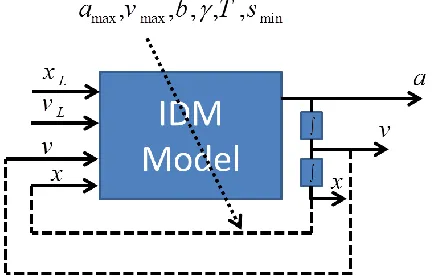
and maximum deceleration (b). In Fig. 1, the block diagram of IDM model is shown.

Figure 1. Block diagram of IDM model

As shown in Fig.1, the block diagram consists of inputs and outputs as well as tuning parameters for the model that shape the behavior of the model. Any change in these six parameters will consequently result to changing the behavior of the modeled vehicle. In case there is provision of vehicles trajectory data, these parameters could hence help in individually modelling the vehicles as well as indicating their differences based on the

parameters. On the other hand, the pre-stated six parameters can be measured which will help in quantifying the differences between the drivers. The above mentioned forms the basis of the contextual concept that acts as the main idea in developing the Heterogeneity Complementary Model (HCM) which is based on IDM model. To develop the mathematical formulation for each parameter using the available trajectory data, there it the need for the assumption that the vehicle trajectory data will be provided which includes the vehicles displacement, velocity and acceleration as well as the headway to preceding car and relative velocity. Therefore, as such, through the use of the above data, the HDM model parameters can be calculated as illustrated below.

Calculation procedure for the parameter maximum acceleration. To calculate maximum acceleration (𝑎_𝑚𝑎𝑥), we need to consider the values of acceleration as a variable and find the maximum value in the update interval. Severally, due to traffic congestion, there is a challenge in finding maximum acceleration, so the most evident value will be the estimated value, but known to be false. The formulation that can be used is:

max

max( )

a



a

(3)

Calculation procedure for the parameter maximum deceleration. The calculation of maximum deceleration (𝑏) is similar to the calculation of 𝑎_𝑚𝑎𝑥. The only difference is that instead of the maximum value of the acceleration, minimum value of acceleration will be chosen as the value for the parameter (b).The formulation that can be used is:

min( )

b



a

(4)

Calculation procedure for the parameter maximum velocity. To calculate the maximum velocity of the vehicle (𝑣_𝑚𝑎𝑥), the velocity curve needs to be calculated by time integration of acceleration and then we can determine the maximum value of the velocity as 𝑣𝑚𝑎𝑥. To

(5)

Mohammad Hossein Noranian, Ahmad Reza Tahsiri

187 International Journal of Transportation Engineering, Vol. 5/ No. 2/ Autumn 2017 acceleration data, some filtering techniques and

data fusion procedures with GPS data need to be applied, which is not in the scope of this paper. The formulation that can be used is:

max

max( )

v



v

(5)

Calculation procedure for velocity form factor.

Calculation of the velocity form factor is a little harder than the above-mentioned parameters. To calculate𝛾, first, the acceleration-velocity plot of the vehicle needs to be plotted as shown in Fig. 2.

For the points depicted in the plot, an envelope curve can be drawn that significantly illustrates the extreme value of acceleration for each fixed value of velocity. It means that maximum acceleration for a certain velocity is shown over the update interval. Based on the curvature of the envelope, a value can be found for the parameter 𝛾 that obeys the relationship indicated below:

max max

1 ( )

a v

d

a v



   (6)

Where “d” is the term which is related to the gap with the leading car and is a disturbance term for the calculation procedure for 𝛾. So the value of 𝛾 can be calculated using the equation below in an update interval. To calculate the 𝛾 parameter,

there is the need to normalize both the acceleration and velocity variables with their maximum values, which results to:

max max

: & :

n n

a v

  ₍₇₎

Therefore, the main model can be reformulated in such a method;

 

2 * max

max 2 *

1

n n

v

s

a

v

s

a

v

s



















































 

  





(8)

In the above equation, the headway related term is always positive due to the square power of the term, so

2 *

0 _n 1 _n ( )

s

a v I

s



 

   

 

  (9)

(6)

Developing a Model of Heterogeneity in Driver’s Behavior

Figure 2. The acceleration-velocity plot and the envelope for the depicted points The overall minimum 𝛾 calculated for all the pairs

in the dataset will be presented as the 𝛾 parameter of the model for the provided information. In can be described in a mathematical formula as:

arg min( 1 )

( , )

n n

a v

for all a v pairs in data set



   

(10)

Calculation procedure for reaction time.

Before presenting a calculation formula for reaction time, on the onset, we need to understand the meaning of the calculation formula. The formula refers to the reaction time as the period in which a driver needs to understand the stimulation from the leading car and reacting to it. For example, the time needed for a driver to understand the leading car is stopping and then decelerating in response to that will be the reaction time. Reaction time can be used in different scenarios but one of the best scenarios is “moving from full stop” stimulation. When vehicles are stopped, and by this time the leading car starts moving, the time difference between the movement start time of leading car and the vehicle is the best measurable estimation in determining the reaction time. In this model, the formulation is developed to find the time difference between the start of the movement for leading vehicle to the vehicle intended. To attain the above, first, there is the need to investigate the position and time at which vehicles are in rest. The formula can be formulated as:

0 &

0

for interval

s

x

x where v

a

t



 

(11)

Based on the above, it hence means that the rest mode for a vehicle is targets the period when the acceleration and velocity of the vehicle are equal to zero for a minimum interval of



t

. As such, the start time of movement can be calculated as:

arg min( ( ) )

m s

t

t  x t x 



x ₍₁₂₎

It therefore means that the start time of movement is defined as the time when the vehicle moves

x



meters from the position where it stopped. Notably, the reasons for defining the



x

bound asserts to the errors in measuring the relative position of cars which need to be considered in computations. By knowing the start time for the leading vehicle and the intended vehicle, the reaction time can be easily calculated:

m m

L

T t t (13)

Calculation procedure for minimum headway.

The minimum headway to the leading car, knowing the above equations, can be easily calculated using:

min

s s

L

s x x (14)

When calculating all the model parameters, each driver’s driving behavior can be described by the set of parameters for IDM model defined as Heterogeneity Vector (HV). Besides, the IDM model can describe the driving behavior of each driver through the knowledge of the set of parameters. Through having these parameters regarding different drivers, in turn, one can understand the differences between drivers’ behavior. The Heterogeneity Complementary Model is depicted in a block diagram scheme in Fig. 3.

(7)

Mohammad Hossein Noranian, Ahmad Reza Tahsiri

189 International Journal of Transportation Engineering, Vol. 5/ No. 2/ Autumn 2017 extended based on the policy determined by the

application.

Figure 3. The heterogeneity complementary model block diagram scheme

The data source will be used to measure heterogeneity among different vehicles traversing a street in a specific interval of time-15 minutes. NGSIM dataset is being used in different studies on microscopic modeling of traffic flow [Abdi, Saffarzadeh and Salehikalam 2016; Poor Arab Moghadam, Pahlavani and Naseralavi 2016;]. Researchers working on the NGSIM program collected the data and extracted the detailed vehicle trajectory data on Lankershim Boulevard in the Universal City neighborhood of Los Angeles, CA, on June 16, 2005. The study area, which consisted of bidirectional data of the three to four lane arterial segments and complete coverage of three signalized intersections, was approximately 500 meters (1,600 feet) in length. The bidirectional data were collected using five video cameras mounted on the roof of a 36-story building located adjacent to the U.S. Highway 101 and Lankershim Boulevard interchange in the Universal City neighborhood. A customized software application developed for both the NGSIM program and NG-VIDEO transcribed the vehicle trajectory data from the

video. These vehicle trajectory data provided the precise location of each vehicle within the study area every one-tenth of a second, resulting in detailed lane positions and locations relative to other vehicles.

A total of 30 minutes of data was available in the full dataset, which was segmented into two 15-minute periods (8:30 a.m. to 8:45 a.m. and 8:45 a.m. to 9:00 a.m.). These periods represented primary congested conditions on the arterial. In addition to the vehicle trajectory data, the Lankershim dataset also contained computer-aided design and geographic information system files, raw and processed videos, aerial ortho-rectified photos ,traffic sign locations and information, windshield videos, weather data, as well as report on aggregate data analysis [FHWA, 2016].

(8)

Developing a Model of Heterogeneity in Driver’s Behavior

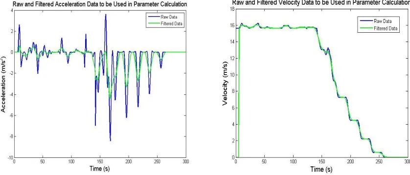
of two HDM parameters which are related to acceleration – maximum acceleration and maximum deceleration. Due to the nature of the information gathered by cameras, the first measured variable is displacement, and velocity and acceleration which will be calculated by deriving the displacement by time. It’s well understood that derivation will increase the power of noise and velocity and acceleration calculated in this framework need to be filtered [Antoniou, 2006]. To filter the velocity, a Finite Impulse Response (FIR) filter with an order of 11 is used to lower the noise contaminations. Besides, the value of acceleration is recalculated using the filtered velocity values [Elliot, 2013]. The above adjustment is used to decrease the noise ratio and on the other hand increase the precision of the parameters which are calculated through the use of the variables. A sample of both raw and filtered value of two aspects that is velocity and acceleration is presented in fig.4. The figure illustrates the differences between the measured raw information and processed information which is used in the calculation procedure for the parameter.

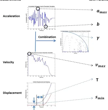
As depicted in fig. 4, there is a notable difference between the value of raw and filtered acceleration data in which will in turn affect the value of IDM parameters. In a bid to clearly illustrate the use of variables such as acceleration, velocity and displacement in calculating the IDM parameters for each driver, there is adoption of a data flow which is portrayed in fig. 5. It is clearly and evidently illustrated that the acceleration and velocity data lead in calculation of four parameters out of the six. The two remaining parameters, that is minimum headway and reaction time, were calculated using vehicle displacement as illustrated in fig. 5.

After adjusting the variables which were used as inputs for HDM, the next step took the lane to applying the HDM formulations with the aim of finding the six parameters which in turn illustrated the differences among drivers. As mentioned below, the Lankershim Street dataset was used and for each 15 minute part of the data set, the HDM model was applied to each driver and the parameter values were extracted. The distribution of calculated parameters is depicted in histogram plot.

(9)

Mohammad Hossein Noranian, Ahmad Reza Tahsiri

191 International Journal of Transportation Engineering, Vol. 5/ No. 2/ Autumn 2017 Figure 5. Data flow in the calculation procedure for the IDM parameters

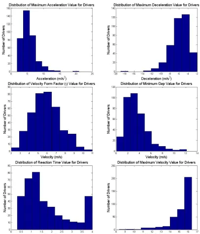
As depicted in the Fig. 6, there is a distribution of values for each parameter which proves the claim that vehicles are behaving differently. Besides, it is evidently depicted that different vehicles embraces different behaviors which initiates the calculation of different values for IDM parameter. However, unlike different values for IDM parameter, fixed value for IDM parameter on the other hand particularly for all the vehicles will consequently cause errors in stimulation that in turn initiates errors in decisions. To compare the homogenous approach with the heterogeneous approach based on the modeling driver behaviors in a quantitate manner, it evident that the fixed value of 4 meters for headway which is assumed in [14] is weakly compatible with the headway

(10)

Developing a Model of Heterogeneity in Driver’s Behavior

NGSIM dataset are being used to simulate the flow in a specific link.

Figure 6. Distribution of IDM parameters for drivers of NGSIM dataset

As portrayed in Fig. 7, each group consists of ten vehicles which did have similar quantity, but had different experienced travel times. Such illustrates the differences in driver behavior that

(11)

Mohammad Hossein Noranian, Ahmad Reza Tahsiri

193 International Journal of Transportation Engineering, Vol. 5/ No. 2/ Autumn 2017 The pre-stated result can proof the claim

grounded on heterogeneity affecting the traffic patterns and relatively calls for the many planning

algorithms which are based on travel time need to consider heterogeneity.

( a )

( b )

(12)

Developing a Model of Heterogeneity in Driver’s Behavior

Figure 7. Simulation of three groups of ten cars passing through the same link. Travel time distribution of each set and the link performance scheme are sketched: (a) first set of heterogeneous vehicles entering a

specific link, (b) second set of heterogeneous vehicles entering the previously specified link, (c) a set of homogenous vehicles entering the link.

5. Conclusion and Future Works

In conclusion, the paper has in detail studied heterogeneity in drivers’ behavior. At first, the paper has presented the IDM model as a microscopic model and its parameters. Besides, the context has introduced a new complementary model in an effort to identify the model parameters from the trajectory data of the vehicle. Related equations and procedures are also defined with the aim of enlightening on the procedure as well as its independence.

As depicted in the simulation results, based on the NGSIM field data, there is a wide range of values for different drivers which brings to light the fact that there is a noticeable difference between the drivers’ behavior which approves the assumption on heterogeneity in the drivers’ behavior. Calculation procedures are also developed to help the model parameter identification in successful extracting required data from the trajectory information.

The entire contribution of the paper can be described as a new modeling approach to heterogeneity in driver’s behavior which is useful in simulating traffic network. Based on the above, it is the first time heterogeneity has been modeled with structured measures to be used in modeling traffic. Besides, the developed model can be widely used in different applications that need to know drivers’ behavior precisely and individually.

One of the possible suggestions for future research is developing a set of equations to relate IDM parameters to variables easily accessible by testing the vehicle and the driver. Variables like vehicle dynamics properties will affect the driver physiologic performance and mental capabilities.

6. References

-Abdi, Ali, Saffarzadeh, Mahmoud and Salehikalam, Arsalan (2016) "Identifying and analyzing stop and go traffic based on asymmetric theory of driving behavior in acceleration and deceleration." International Journal of Transportation Engineereing, Vol. 3, No. 4, pp. 237-251.

-Ahmed, Kazi Iftekhar (1999) "Modeling drivers' acceleration and lane changing behavior." PhD diss., Massachusetts Institute of Technology.

-Alexiadis, Vassili, James Colyar, John Halkias, Rob Hranac, and Gene McHale (2004) "The next generation simulation program." Institute of Transportation Engineers. ITE Journal Vol. 74, no. 8, pp. 22.

-Antoniou, Andreas (2006) ”Digital signal processing”. Toronto, Canada: McGraw-Hill.

-Chen, Chao, Alexander Skabardonis, and Pravin Varaiya (2003) "Travel-time reliability as a measure of service." Transportation Research Record: Journal of the Transportation Research Board, Vol. 1855, pp. 74-79.

-Dang, Shuping, Zeqi Hong, Sen Yang, and Liam Baker (2013) "Intelligent urban traffic management system based on the energy-circle cards platform." In Information Science, Electronics and Electrical Engineering (ISEEE), 2014 International Conference on, vol. 1, pp. 457-459.

-Guo, Xiaolei, and Henry X. Liu (2011) "Bounded rationality and irreversible network change." Transportation Research Part B: Methodological Vol.45, No.10, pp. 1606-1618.

-Hakamies-Blomqvist, Liisa, Sirén, Anu, and Davidse, Ragnhild (2004). “Older drivers: a review”. Väg-och transportforskningsinstitutet.

(13)

Mohammad Hossein Noranian, Ahmad Reza Tahsiri

195 International Journal of Transportation Engineering, Vol. 5/ No. 2/ Autumn 2017 using microscopic data." Transportation Research

Record: Journal of the Transportation Research Board Vol. 2188, pp. 37-45.

-Kesting, Arne, Treiber, Martin Schönhof, Maring and Helbing, Dirk (2007) "Extending adaptive cruise control to adaptive driving strategies." Transportation Research Record: Journal of the Transportation Research Board, No. 2000, pp 16-24.

-Krajzewicz, Daniel, Reinhart Kühne, and Peter Wagner (2004) "A Car Driver´ s Cognition Model." Proceedings of Intelligent Transportation Systems Safety and Security Conference. Vol. 400.

-Leduc, Guillaume (2008) "Road traffic data: Collection methods and applications." Working Papers on Energy, Transport and Climate Change 1. No. 55.

-Liu, YanFei, and ZhaoHui, Wu (2007) "Improvement of ACT-R for modeling of parallel and multiprocessing driver behavior." International Journal of Intelligent Control and Systems Vol.12, No.1, pp.72-81.

-Lo, Hong K., Elbert Chang and Yiu, Cho Chan (2001) "Dynamic network traffic control." Transportation Research Part A: Policy and Practice Vol. 35, No. 8, pp. 721-744.

-Manolis, Diamantis (2016) "Automated tuning of ITS management and control systems: Results from real-life experiments." Transportation Research Part C: Emerging Technologies Vol. 66, pp. 119-135.

-Poor Arab Moghadam, M., Pahlavani, P. and Naseralavi, S. (2016) “Prediction of car following behavior based on the instantaneous reaction time using an ANFIS-CART based model”, International Journal of Transportation Engineering, Vol. 4, No. 2, pp.109-126.

-Salvucci, Dario D. (2006) "Modeling driver behavior in a cognitive architecture", Human Factors: The Journal of the Human Factors and Ergonomics Society Vol. 48, No. 2, pp. 362-380.

-Tang, Tieqiao, Weifung, Shi; Huayan, Shang, Yunpeng, Shang … (2014) "A new car-following model with consideration of inter-vehicle communication." Nonlinear Dynamics, Vol. 76, No. 4, pp. 2017-2023.

-Toledo, Tomer, Haris N. Koutsopoulos and Ben-Akiva, Moshe (2009) "Estimation of an integrated driving behavior model." Transportation Research Part C: Emerging Technologies Vol. 17, No. 4, pp. 365-380.

-Treiber, Martin and Helbing, Dirk (1999) "Macroscopic simulation of widely scattered synchronized traffic states." Journal of Physics A: Mathematical and General Vol. 32, number 1, L17.

-Treiber, M.; Hennecke, A. and Helbing, D. (2000) "Congested traffic states in empirical observations and microscopic simulations", Physical Review E, Vol. 62, No.2, pp. 1805.

-Web page

http://www.fhwa.dot.gov/publications/publicroa ds/07jan/01.cfm visited at 2016/12/01

-Zhao, Dongbin; Yujie Dai, and Zhang, Zhen (2012) "Computational intelligence in urban traffic signal control: A survey." IEEE Transactions on Systems, Man, and Cybernetics, Part C (Applications and Reviews) Vol.42, No. 4, pp. 485-494.