Franck BOYER, Thierry GALLOUET, Rapha`ele HERBIN and Florence HUBERT Editors
NUMERICAL SIMULATION OF TWO-PHASE MULTICOMPONENT FLOW
WITH REACTIVE TRANSPORT IN POROUS MEDIA: APPLICATION TO
GEOLOGICAL SEQUESTRATION OF CO
2∗Etienne AHUSBORDE
1, Michel KERN
2and Viatcheslav VOSTRIKOV
3Dedicated to Amaia, for a long and happy life
Abstract. In this work, we consider two-phase multicomponent flow in heterogeneous porous media with chemical reactions. Equations governing the system are the mass conservation law for each species, together with Darcy’s law and complementary equations such as the capillary pressure law. Coupling with chemistry occurs through reactions rates. These rates can either be given non-linear functions of concentrations in the case of kinetic chemical reactions or are unknown in the case of equilibrium chemical reactions (such as reactions in aqueous phase). In this latter case, each reaction gives rise to a mass action law, an algebraic relation that relates the activities of the implied species. The resulting system will couple partial differential equations with algebraic equations. The aim of this paper is to develop a numerical method for the simulation of this system. We consider a sequential approach that consists in splitting the initial problem into two sub-systems. The first subsystem is a two-phase two-component flow, while the second subsystem is devoted to a reactive transport problem. For the two-phase two-component flow part, we have used an already existing module of the open-source parallel multiphase flow simulator DuMuX. To solve the reactive transport problem, we have implemented a new module in the DuMuXframework that solves a single phase multicomponent transport problem, and we have coupled it with a locally developed code for chemical equilibrium, called ChemEqLib, through a sequential iterative approach. Then, both modules have been coupled to propose a simple, but mathematically consistent, iterative method that handles two-phase flow with reactive transport. The approach is validated on a 2D example from the literature representative of a model for the long-term fate of sequestered CO2.
Introduction
Carbon Capture and Storage (CCS) is seen as one of the ways to mitigate the effects of global warming, and assessing the viability of geological storage must rely on numerical simulations, if only because of the long time scales involved. Several physical and geochemical trapping mechanisms must be combined to ensure a
∗ This research has been supported by the Conseil R´egional d’Aquitaine, and the CEA-INSTN. Their support is gratefully
acknowledged.
1 LMA Pau UMR 5142, Bˆatiment IPRA - UPPA, Avenue de l’Universit´e - BP 1155, 64013 Pau Cedex
2 INRIA, CRI Paris–Rocquencourt, BP 105, 78153 Le Chesnay Cedex & Maison de la Simulation, Digiteo Labs, CEA Saclay,
91191 Gif-sur-Yvette Cedex
3LMA Pau UMR 5142, Bˆatiment IPRA - UPPA, Avenue de l’Universit´e - BP 1155, 64013 Pau Cedex & Maison de la Simulation, Digiteo Labs, CEA Saclay, 91191 Gif-sur-Yvette Cedex
c
EDP Sciences, SMAI 2015
high containment rate, and geochemical chemical trapping becomes increasingly important over longer time scales [18]: carbon dissolution in water occurs over hundreds of years, and formation of carbonate minerals over millions of years, see [21].
The physical description of CO2 geological storage rests on underground flow of water and CO2, both in aqueous and gaseous phases, as well as chemical interactions between them and the surrounding rock matrix, and other dissolved chemical species. From the numerical point of view, this task requires the solution of a large coupled system of partial differential equations (describing two-phase compositional flow), together with algebraic or ordinary differential equations modelling chemical reactions. This paper presents a numerical method to simulate such a system .
Both (compositional) multiphase flow and geochemical transport have been the subject of numerous studies, some of which are recalled below. More recently, codes targeting coupled two-phase flow and reactive transport have appeared. Several such codes are described in the book edited by Zhang et al.[31], and two more recent references are the papers by Saaltinket al.[25] and Fanet al. [12].
As usual for coupled problems, the coupling between flow, transport and chemistry can be treated in one of two ways. In a fully coupled procedure, one nonlinear system gathering all equations is solved at each time step. This is the approach adopted in [12] and also in [25]. But, even though both works do solve the fully coupled problem, they do not couple two different codes. Rather, they add chemical equations to an existing, sophisticated two-phase flow solver. In the case of [12], the chemical equations are solved together with the conservation laws for flow and transport. In the case of [25], however, the solution of the chemical problem is pre-computed for some number of reference conditions (they are shown to depend only on gas pressure), and then polynomial interpolation is used within the solution procedure, leading to a large reduction in computing time.
Given the complexity of the chemistry codes, it may not be surprising that most studies using such type of codes have instead focused on the sequential solution approach, where flow and reactive transport (or possibly, flow, transport and chemistry) are solved sequentially at each time step, possibly within an iterative loop. This is in particular the case for the codes described in [31], such as [15], [16], [27] and [29]. No comparative study exists yet to quantify the accuracy loss for this approach, but its gain in implementation and saving in computing time are fairly obvious. This is the approach we have chosen to follow in this paper.
An outline for the rest of the paper is as follows: we detail the physical model for two-phase, multicomponent flow, with reactive transport in section 1. The sequential strategy is described in section 2, both in a general setting and as it applies to the specific case of CO2 sequestration. Section 3 contains a description of the simulator, as well as its application to a test case taken from [25].
1.
Mathematical and physical model
1.1.
Chemical equations
We consider a set ofNschemical species (Yj)j=1...Ns linked byNr equilibrium reactions:
Ns
X
j=1
SijYj 0, i= 1, . . . , Nr⇐⇒SY 0,
where S ∈ RNs×Nr is the stoichiometric matrix. Each reaction gives rise to a mass action law that links the activities of the species. In this work, we assume that all aqueous species have ideal activity (that is, activity equals concentration), whereas solid species have (by convention) their activity equal to 1. When written in logarithmic form, the mass action law becomes linear and takes the form
where a is a vector of activities and fugacities of all chemical species,K is a vector of equilibrium constants, and we have used the convention that logais the vector with components logai for any vectorawith positive componentsai.
We follow the Morel formalism [20], and split the set of all chemical species into primary and secondary species. If we assume that the stoichiometric matrix has full rank (there are no redundant reactions), it can then be transformed to the form:
S= (−I ˜S), (2)
so that each chemical reaction expresses the formation of a single secondary species from the set of primary species.
In addition to the mass action law, each primary species gives rise to a conservation equation that expresses how its given total concentration is distributed among the species itself and the secondary species. The mass conservation law is written as follows:
cp+ ˜STcs=T, (3)
wherecpandcs are the vectors of concentrations of primary and secondary species and the total concentration
T is known (see next section).
Solving the chemical equilibrium problem consists in solving the non-linear system that couples equations (1) and (3).
1.2.
Mathematical model for two-phase multicomponent flow with reactive transport
In the sequel, the index α ∈ {l, g, s} (l for liquid, g for gas ands for solid) refers to the phase, while the superscriptirefers to the species. To specify which species belongs to which phase, we define thephase – species
correspondence by settingαi to the index of the phase that contains speciesi(see an example in section 2.2). For each species, in its phase, we consider the mass balance equation (see for instance [17]):
∂ ∂t(θαic
i)− ∇ ·(θ
αiDαi∇ci) +∇ ·(ci−→qαi) =
X
j
Sjirj, i= 1. . . Ns, (4)
where θα[-] denotes the volumetric content of phaseα(θα=φSα, φ[-] being the porosity of the medium and
Sα [-] the saturation of phaseα ifα∈ {l, g,} and θs= 1), ci [kg.m−3] is the mass concentration of species i (in phaseαi), Dα [m2.s−1] denotes the diffusivity of phaseα, −→qα [m.s−1] is the Darcy velocity of phase α, rj [kg.m−3.s−1] is the rate of reactionj and
Sji[-] is the stoichiometric coefficient of speciesiin reactionj. Note that we have made the simplifying (but essential for the decoupling procedure) assumption that the diffusion coefficient is independant of the chemical speciesi.
The Darcy velocity of phaseαis expressed as follows:
− →
qα=−
krα
µαK
(∇Pα−ρα−→g), (5)
wherekrα(Sl) [-] denotes the relative permeability of phaseα,µα [Pa.s] is the dynamic viscosity of phaseα,K [m2] is the absolute permeability tensor, P
α [Pa] is the pressure of phaseα, ρα [kg.m−3] is density of phaseα and−→g [m.s−2] is the gravitational acceleration.
The phase pressures are connected by the capillary pressure law:
Pc(Sl) =Pg−Pl. (6)
To simplify notation, we introduce the diffusion-advection operator:
We add that, since the mobile phase is immobile, Ds= 0 and −→qs = − →
0 , so thatLs(.) = 0.
In this work we assume that all reactions are at equilibrium, that is that the reaction rates are much faster than the rate implied by flow and transport. This assumption is certainly valid for reactions in the aqueous phase, or for the dissolution of gaseous CO2, but may be less justified for reactions involving minerals. Then, the reaction ratesrj are unknown. They can be eliminated by multiplying equation (4) by a (Ns−Nr)×Nr component matrixU such thatUST = 0. This matrix exists because of the full rank assumption on
S. When S is put in the special form (2), the component matrix U is simply U = ( ˜ST I). In general, the computation of U can be performed in different ways (see for instance [23]), the simplest being Gaussian elimination.
After multiplication byU, equation (4) becomes:
X
α
∂
∂t(θαC
k
α) +Lα(C k α)
= 0, k= 1, . . . , Ns−Nr, (8)
with
Cαk=
X
istαi=α
Ukici, k= 1, . . . , Ns−Nr, α∈ {l, g, s}. (9)
To complete this new reduced set of equations and obtain the same number of equations as there are unknowns, we add theNr mass actions laws defined by (1).
In the next section, we present our methodology to solve this new system composed of mass actions laws (1) and mass conservations laws (8).
2.
Solution methodology
In the literature, there are two main kinds of approaches for the numerical simulation of two-phase multi-component flow with reactive transport in porous media. The first one is a fully-coupled approach that solves the full system of equations (1)-(8) simultaneously (see for instance [12]). The second one is a sequential approach (see for instance [24, 28]) and is applicable if the following conditions are satisfied:
• Among the chemical species there exists one dominant species within each phase, • Various phase states of the dominant species are in chemical equilibrium,
• The presence of other chemical species has no significant influence on the mass balance equations of the dominant species.
In this case, the solution process can be divided into two steps. In the first step, we consider a simplified two-phase two-component flow only governed by the dominant species and chemical reactions are neglected. In the second step, we consider a reactive transport problem for the other minor species using quantities computed at the first step.
In this work, we use this kind of sequential approach. In the rest of this section, we make our strategy precise.
2.1.
Sequential strategy
The general idea of the sequential approach is to separate the system of equations into two subsystems, the first one devoted to a two-phase two-component flow and the second one devoted to the reactive transport problem. In the sequel,cddenotes the vector of concentrations of the dominant species in their potential various phase states while cm is the vector of concentrations of the minor species. The choice of dominant species is arbitrary, provided they satisfy the hypothesis outlined below, but in practice will be based on the expected properties of the system being studied. This is exemplified for a H2O-CO2 system in section 2.2.
We make the following assumptions:
• We assume that the state equation for density depends only on the pressures and concentrations of dominant species.
2.1.1. Two-phase two-component flow
In this step we compute cd, ρα, Pα, Sα and −→qα. To do this, we consider equations (8) only for dominant species, the contribution from the minor ones being treated explicitly. To close the system, we add the mass action laws involving the dominant species and their potential various phase states. Note that we consider that interphase exchange relations, like Henry’s or Raoult’s law, are included in the mass action laws. In practice, this means that we are solving a two-phase, two-component flow, see section 3.1.1.
2.1.2. Reactive transport
Once the two-phase two-component flow has been computed, we can solve the reactive transport problem, given cd,ρα,Pα, Sα and−q→α, to obtaincm. This problem consists of equations (8) for minor species and mass action laws defined by (1) that have not been taken into account in the two-phase two-component flow. Once
cmis computed, the porosity can be updated thank to the relation:
φ= 1−θmin, (10)
where θmin [-] is the mineral volumetric content. The mineral volumetric content is a function of the concen-trations of the solid species and therefore depends on cm. Moreover, the contribution of minor species in the equations (8) of the dominant species can be updated.
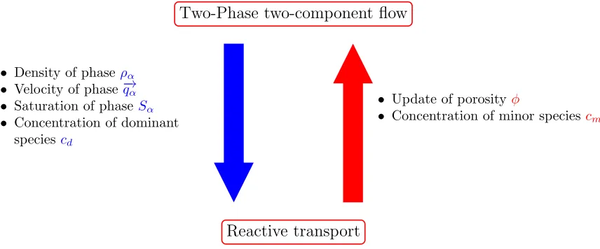
To summarize, our methodology for the coupling is illustrated in figure 1.
Two-Phase two-component flow
Reactive transport
• Density of phaseρα • Velocity of phase−q→α • Saturation of phaseSα • Concentration of dominant
speciescd
• Update of porosityφ
• Concentration of minor speciescm
Figure 1. Coupling procedure between flow and reactive transport modules.
2.2.
Application to CO
2Storage
Liquid phase (l) Gaseous phase (g) Solid phase (s) H2O, CO2(l), H+, CO2(g) CaCO3 OH–, HCO3–, Ca2+
Table 1. Chemical species.
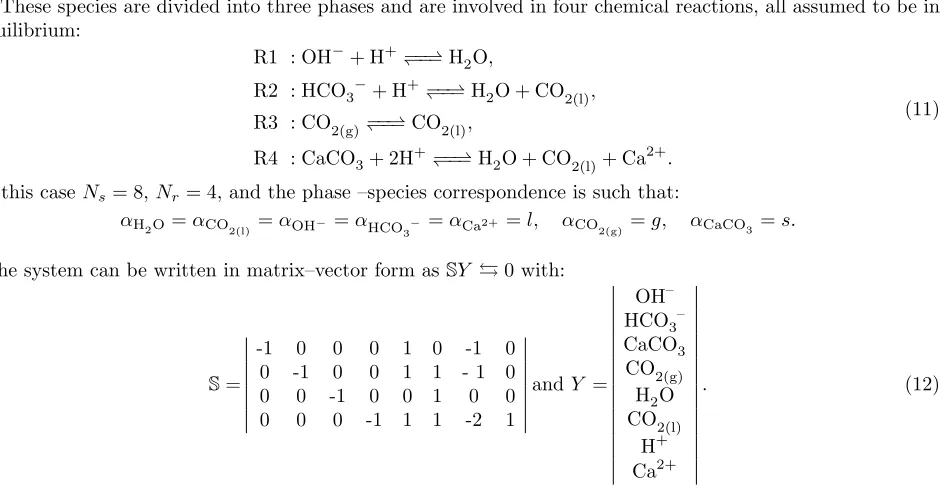
These species are divided into three phases and are involved in four chemical reactions, all assumed to be in equilibrium:
R1 : OH−+ H+−−)−−*H2O,
R2 : HCO3−+ H+−−)−−*H2O + CO2(l),
R3 : CO2(g) −−)−−*CO2(l),
R4 : CaCO3+ 2H+−−)−−*H2O + CO2(l)+ Ca2+.
(11)
In this case Ns= 8, Nr= 4, and the phase –species correspondence is such that:
αH2O=αCO
2(l) =αOH−=αHCO3
− =αCa2+=l, αCO
2(g) =g, αCaCO3 =s.
The system can be written in matrix–vector form as SY 0 with:
S=
-1 0 0 0 1 0 -1 0 0 -1 0 0 1 1 - 1 0 0 0 -1 0 0 1 0 0 0 0 0 -1 1 1 -2 1
andY = OH– HCO3– CaCO3
CO2(g) H2O CO2(l)
H+ Ca2+
. (12)
Note that Sis already in the special form pointed out in section 1.1, so that the component matrix U can be read off directly fromS.
For each species in each phase, equation (4) writes:
H2O : ∂
∂t(θlc
H2O) +L
l(cH2O) =rOH−+rCaCO
3+rHCO3
−,
CO2(l) : ∂
∂t(θlc CO2(l)
) +Ll(cCO2(l)) =r
HCO3−+rCO2(g)+rCaCO3,
H+ : ∂ ∂t(θlc
H+) +L
l(cH +
) =−rOH−−2rCaCO
3−rHCO3
−,
Ca2+ : ∂
∂t(θlc Ca2+
) +Ll(cCa2+) =rCaCO3,
HCO3−: ∂
∂t(θlc
HCO3−) +Ll(cHCO3−) =−r HCO3−,
OH− : ∂
∂t(θlc
OH−) +Ll(cOH−) =−r OH−,
CO2(g) : ∂
∂t(θgc CO2(g)
) +Lg(cCO2(g)) =−rCO 2(g),
CaCO3 : ∂
∂tc
CaCO3 =−r
Multiplying this system by the matrixUintroduced previously is equivalent to performing linear combinations on its rows, so as to eliminate the equilibrium rates and reduce the number of equations fromNstoNs−Nr:
∂ ∂t(θlC
H2O
l +C
H2O
s ) +Ll(C
H2O
l ) = 0,
withCH2O l =c
H2O+cOH−+cHCO3− andCH2O
s =cCaCO3,
∂ ∂t(θlC
CO2(l)
l +θgC
CO2(l)
g +C
CO2(l)
s ) +Ll(C
CO2(l)
l ) +Lg(C
CO2(l)
g ) = 0,
withCCO2(l) l =c
CO2(l)
+cHCO3
−
, CCO2(l)
g =cCO2(g) andC
CO2(l)
s =cCaCO3,
∂ ∂t(θlC
H+
l +C
H+
s ) +Ll(C
H+
l ) = 0,
withCH
+ l =c
H+−cOH−−cHCO3− andCH+
s =−2cCaCO3,
∂ ∂t(θlC
Ca2+ l +C
Ca2+
s ) +Ll(CCa2+) = 0, (13)
withClCa2+ =cCa2+ andCsCa2+=cCaCO3.
To recover a total number of equations equal toNs, we addNr mass action laws:
γ(cCO2(g), Pg) =cCO2(l),
cOH− =KOH−cH
+
,
cHCO3
−
=KHCO
3
−cCO2(l)(cH
+ )−1,
1 =KCaCO3c CO2(l)
cCa2+(cH+)−2. (14)
In (14), for CO2(g) the activity γ is a function of cCO2(g) and the gas pressure Pg. For the aqueous species OH– and HCO3–, we use a model of ideal activity that considers activity equal to the concentration, and by convention the activity of water is taken to be equal to 1. Finally, for CaCO3, the activity is taken as a constant and equal to 1.
Now, we assume that in each phase, there exists a dominant species (H2O in liquid phase and CO2(g) in gas phase) and that the other minor species do not affect much the flow. In this case:
cd=
cH2O cCO2(l)
cCO2(g)
andcm=
cH+ cCa2+
cOH− cHCO3− cCaCO3
. (15)
Our strategy consists in solving sequentially:
• a simplified two-phase two-component flow system for H2O–CO2 to compute pressures Pα, velocities −
→
qα, saturationsSα and the concentrations of the dominant speciescd,
Consequently, the set of equations (13,14) is split into two subsets. The first one is devoted to the two-phase two-component flow:
∂ ∂t(θlc
H2O) +Ll(cH2O) = Ψ 1(cOH
− , cHCO3
−
, cCaCO3),
∂ ∂t(θlc
CO2(l)
+θgc
CO2(g)
) +Ll(c
CO2(l)
) +Lg(c
CO2(g)
) = Ψ2(cHCO3
−
, cCaCO3),
γ(cCO2(g), P g) =c
CO2(l) ,
with
Ψ1(cOH
− , cHCO3
−
, cCaCO3) =−∂
∂t
θl(cOH−+cHCO3
−
) +cCaCO3
−Ll(cOH−+cHCO3
−
),
and
Ψ2(cHCO3
−
, cCaCO3) =−∂
∂t
θlcHCO3
−
+cCaCO3
−Ll
cHCO3
−
The second subset is devoted to the reactive transport problem and is computed by solving the system:
∂ ∂t(θlC
H+
l +C
H+
s ) +Ll(C
H+
l ) = 0,
∂ ∂t(θlC
Ca2+
l +C
Ca2+
s ) +Ll(CCa2+) = 0,
cOH− =KOH−cH
+
,
cHCO3
−
=KHCO
3
−cCO2(l)(cH
+ )−1,
1 =KCaCO3c CO2(l)
cCa2+(cH+)−2.
These two subsystems are solved sequentially. First, the computation of the two-phase two component flow is performed, with the contribution of the minor species (i.e. functions Ψ1 and Ψ2) treated explicitly, so as
to uncouple the two steps. Then, the reactive transport problem is solved using quantities from the first step. Finally, concentrations of minor speciescmare used to update the porosity (see eq. (10)) as well as the functions Ψ1and Ψ2.
In the next section, we present our numerical methodology to solve our sequential approach.
3.
Numerical simulation
3.1.
Simulator
Our methodology has been implemented in DuMuX(DUNE for Multi-{Phase, Component, Scale, Physics, ...} flow and transport in porous media) [2, 13], a free and open-source simulator for flow and transport processes in porous media, based on the Distributed and Unified Numerics Environment DUNE [3].
3.1.1. Two-phase two-component flow
In this model, the principal difficulty consists in taking into account the possible appearance and disappear-ance of a phase. This process is managed by a phase state dependent variable switch. Three different cases can be distinguished:
• Liquid and gas phases are present: liquid pressure Pl and a saturation are used (either Sl or Sg), as long as 0< Sα<1.
• Only liquid phase is present: liquid pressurePland the mass fraction of CO2in the liquid phaseX CO2
l are used, as long as the maximum mass fraction is not exceeded (XCO2
l < X
CO2
l,max).
• Only gas phase is present: liquid pressurePland the mass fraction of H2O in the gas phase,X H2O
g are used, as long as the maximum mass fraction is not exceeded (XH2O
g < X
H2O
g,max).
3.1.2. Reactive transport
For the reactive transport problem, we have first implemented in DuMuX a one-phase multicomponent transport model. As starting point we used the single-phase, two-component model already implemented in DuMuX. This model implements a one-phase flow of a compressible fluid, that consists of two components. The primary variables are the pressurepand the mole or mass fraction of dissolved componentsx. In our model, we want to impose the velocity and consequently the pressure. So, we have first removed the pressure from the set of primary variables. Then, we have increased the number of dissolved components from two to N. We have named this new model 1pN cfor one-phase N-component.
The last component is a locally developed code for chemical equilibrium called ChemEqLib [1, 5]. This code solves the chemical equilibrium problem that consists of mass actions laws and mass conservation laws. The proposed formulation can involve both homogeneous (aqueous complexation) and heterogeneous reactions (mineral dissolution/precipitation and ion exchange). For minerals, one does not know a priori which species are in the solid form, and which are dissolved, leading to a system of equations that is of complementarity type. In the ChemEqLib code, this is handled by an outer loop over the possibly dissolved mineral species, and a check as to whether the included species are not over- or under-saturated (see [6]). At each of these outer iteration, a non-linear system is solved using a globally convergent Powell’s hybrid method.
To solve the reactive transport subsystem, we have coupled the 1pN cand ChemEqLib codes. The reactive transport problem can be written as follows:
∂(φSlCl)
∂t + ∂Cs
∂t +Ll(Cl) = 0,
T =φSlCl+Cs,
Cs= ΨC(T), (16)
whereClis the vector of the total concentration of liquid species whileCsis the vector of the total concentration of solid species. Equation (16) corresponds to the resolution of the chemical equilibrium. In the literature, many approaches have been proposed to solve reactive transport problem. Sequential approaches (see for instance [10,30]) consists in solving sequentially the transport and chemical reactions. In the direct substitution approaches, the equation of chemistry are directly substituted in the equations of transport. This can be done explicitly as in [14] or implicitly as in [19, 23] or [4]. The problem can also be reformulated as a differential algebraic system (DAE) as in [11].
SupposingCn l, C
n+1,k l , C
n
s, Csn+1,k, S n+1
l , S n l, φ
nare known,Tn+1,k+1, Cn+1,k+1
s , C n+1,k+1
l are computed thanks to the following iterative scheme:
φnS
n+1
l C n+1,k+1
l −SlnCln
∆t +
Cn+1,k s −Csn
∆t +Ll(C
n+1,k+1
l ) = 0,
Tn+1,k+1=φnSln+1Cln+1,k+1+Csn+1,k,
Csn+1,k+1= ΨC(Tn+1,k+1).
whereφnis an approximation of the porosity computed at timen∆t,Sn+1
l andSndenote approximations of the saturations respectively at time (n+ 1)∆tandn∆t. For the other quantities we used the following convention:
Cln,k denotes the approximation of quantityCl at time n∆tand at iteration kin the iterative loop of the SIA algorithm.
The algorithm is stopped when:
||Cln+1,k+1−Cln+1,k|| ||Cln+1,k+1|| +
||Cn+1,k+1
s −Csn+1,k|| ||Csn+1,k+1||
< ,
where||.||is a discrete L2norm, and is a given tolerance (1).
Note that all terms coming from the flow subsystem are treated explicitly. Even thoughSln+1 appears, this is a known quantity that has been computed in the flow stage. The same applies for the term φn: we do not re-evaluate the porosity during the reactive transport step.
3.2.
Application Example
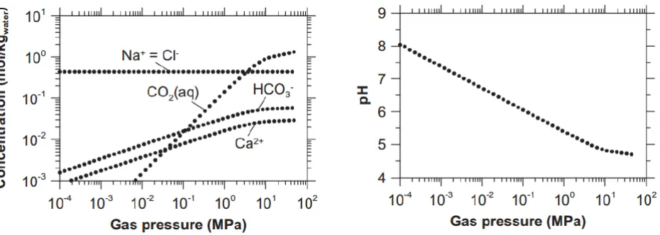
To validate our methodology, we have carried out a test introduced by Saaltinket al. in [25]. The authors of this article elaborate a coupled physical model of two-phase multicomponent flow and construct a numerical simulator that solves the entire system using a fully-coupled approach. To reduce the complexity of the consid-ered numerical task, the authors chose a simplified method for computing chemical equilibrium states, whereas in our case the full nonlinear system for equilibrium is solved. Instead of solving a system of mass action laws coupled with expression of total concentrations (section 1.1), the authors of [25] use a pre-calculated tabulated function that returns the concentrations of all species at chemical equilibrium according to the value of gas pressure. This choice simplifies the computation and reduces computing time. However, it created a difficulty for reproducing the test conditions. The functions for important chemical species are presented as graphs (see Figure 1 in [25]). For convenience, we have reproduced this illustration in Figure 2.
3.2.1. Definition of the test
The domain is an axisymmetric 2D geometry of 100 m thickness, representing a horizontal aquifer at 1500 m depth. The domain extends to 5 km laterally and an injection well with a radius of 0.15 m is located at the centre of the domain.
The chemical system coincides with the one introduced in table 1. Temperature of the reservoir is constant and equal to T = 333 K. The equilibrium constants for the reactions are shown in table 2. As previously mentioned, the values were computed from the graphs of primary species concentration in Figure 2, and for this reason can slightly differ from the values actually used in [25].
Constitutive laws and physical parameters are given in table 3. Initial porosity is equal to 0.1.
As initial conditions for the two-phase two-component H2O-CO2 flow we have used hydrostatic condition for liquid pressurePl, initial liquid saturationSl= 1 and initial CO2concentration in liquid phase equals 1.223 10−4
mol.l−1. Initial conditions for the reactive transport problem are shown in table 4. Because in the article [25],
Figure 2. Concentrations of the most important chemical species (CO2(l), HCO3 –, Ca2+
, Cl–) and pH as a function of gas pressure. Taken from [25].
H2O H+ CO2(l) Ca2+ logK
OH– 1 -1 0 0 -14
HCO3– 1 -1 1 0 -5.928
CaCO3 1 -2 1 1 -8.094
Total TH2O TH+ TCO
2(l) TCa2+ Table 2. Morel’s table.
their values at initial time. Consequently, these values were read off the graph in Figure 2 with an initial gas pressure equal to 10−3MPa.
An additional difficulty caused by the choice of a sequential procedure is that we need to prescribe separate boundary conditions for the two sub-problems. For the two-phase two-component H2O-CO2flow, a prescribed CO2 mass flow rate (2.5 Mt.year−1) is imposed at the injection well, no flow conditions are imposed at the
upper and lower parts of the domain and finally, a constant pressure is enforced at the outer boundary. For the reactive transport problem, a Dirichlet boundary condition equal to the initial condition is imposed for the concentrations, impermeable Neumann boundary conditions are enforced at the upper and lower parts of the domain and an outflow boundary condition is applied at the outlet.
3.2.2. Numerical results
The period of simulation is equal to 1 year. In [25], the authors used a two-dimensional mesh containing 6600 elements. The size of the elements is 5m close to the injection well while it increases up to 30m close to the outer boundary. It is impossible for us to deal with the same mesh so we have used a mesh with a constant step size equal to the finest size in [25], that is 5m. Our corresponding mesh contains 10000 elements (500×20). For the time step management, DuMuX adapts automatically the time step according to the number of iterations needed in the Newton scheme to solve the non-linear problem. For this test case, we fixed the maximal time step equal to 1 day. This choice will be justified in section 3.2.3.
Constitutive law Parameters Retention curve (capillary pressure law)
Sl= 1 +
P
g−Pl
P0
1−1m!
−m
P0= 0.02 MPa m= 0.8 Darcy’s law
− →
qα=−
krα
µα
K(∇Pα−ρα→−g), α=l, g −→g =
0 −9.81
0
, K= 10−13Im2
Relative permeability
krα=Sαn, α=l, g n= 1
Liquid diffusion/dispersion tensor
Dl=DmI+dL|−→ql|+ (dL−dT) − →q
l−→qlt |−→ql|2
Dm= 1.6 10−8 m2.s−1
dL= 5 m
dT = 0.5 m Solid density
ρs= 2700 kg.m−3 Porosity
φ= 1−cCaCO3MCaCO3
ρs
MCaCO3 = 0.1 kg.mol−1
Liquid density
ρl=ρl0exp(αT +β(Pl−Pl0) +γS) α=−3.4 10−4K−1 β = 4.5 10−4 MPa−1
T = 333 K, S= 0.025
ρl0= 1037.12 kg.m−3 Pl0= 0.1 MPa, γ= 0.19
Liquid viscosity
µl= 4.8 10−4 Pa.s Gas density
ρg is tabulated variable. Tabulated values are calculated by the model described in [26]
Gas viscosity
µg=µ0
4 X i=1 1 X j=0 aijρiR
TRj
ρR=ρg/ρcr
TR=T /Tcr
µ0=TR0.5
27.22−16.63
TR
+4.67
T2
R
µPa.s
ρcr= 468 kg.m−3
Tcr= 304 K
T = 333 K
a10= 0.249, a11= 0.00489 a20=−0.373, a21= 1.23 a30= 0.364, a31=−0.774 a40=−0.0639, a41= 0.143
Table 3. Physical parameters for test case.
conc. total conc. total liquid conc. total solid conc. H+ 4.081 10−8 −48.6 −3.503 10−3 −48.6
Ca2+ 1.708 10−3 24.3 1.708 10−3 24.3
Table 4. Initial conditions for reactive transport problem (in mol.l−1).
Figure 3. Liquid saturationSl after 100 days and 1 year of CO2 injection. Only the 1.1 km
closest to the injection is presented.
of the gas pressure evolution coincide, but the computed maximum values are different (a difference of 6.5% is observed). A possible explanation is the difference between the models used in both simulation. For instance in [25], the effects of dissolution of calcite are taken into account to change the porosity and the permeability while in our case, only the porosity is modified and the permeability remains constant.
Figure 4. Gas pressurePgafter 100 days and 1 year of CO2injection. Only the 1.1 km closest
to the injection is presented.
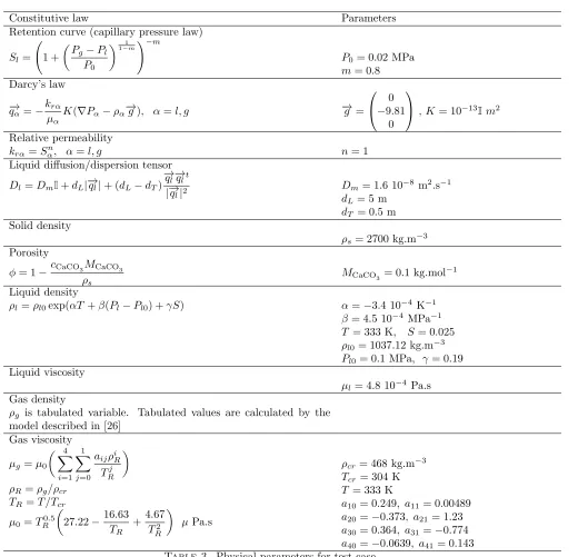
vertical dispersion of the liquid CO2and by a vertical downward flux due to denser CO2saturated liquid phase being on top of a lighter non-saturated zone.
Figure 5. Liquid density ρl after 100 days and 1 year of CO2 injection. Only the 1.1 km
closest to the injection is presented.
Figure 6 represents the precipitation/dissolution of calcite after 100 days of injection of CO2. In the vicinity of CO2, the calcite is dissolved. Calcite dissolves in zones where the liquid phase contains dissolved carbon dioxide reacting with mineral calcite. The amount of dissolved calcite is maximal close to the injection border and gradually decreases as the boundary of the liquid CO2 plume is approached. Although the same trend is observed in both simulations, the actual amount of dissolved calcite inside of gaseous CO2 differs from that obtained in [25]. To better see the difference we give a more precise comparison of the simulations in Figure 7, by showing a graph of precipitated/dissolved calcite volume fraction after 100 days of CO2 injection at two depths as a function of distance from the left side of the domain. We observe that the quantity of dissolved calcite decreases with the distance to the left border. The shapes of both graphs obtained in our simulation and from the results of [25] are similar, but the actual values are different. This difference can be explained by the possibly different values of the equilibrium constants, as noted in section 3.2.1.
Figure 6. Precipitated/dissolved calcite volume fraction after 100 days of CO2injection. Only the 1.1 km closest to the injection is presented.
Figure 7. Precipitated/dissolved calcite volume fraction after 100 days of CO2 injection at two depths (depth equals 10 m on the left and 50 m on the right). Red lines represent obtained results. Blue lines represent M. W. Saaltink’s results. Dissolution is indicated by negative values.
Figure 8. Gas pressure evolution at a point placed 200 m away from the injection well and 25 m below the top of the aquifer. Red line represents obtained results. Blue line represents M. W. Saaltink’s results.
3.2.3. Convergence analysis
To check the convergence of the solution in time, we have compared in figure 10 the precipitation/dissolution of calcite after 100 days of injection of CO2, for different time steps (12 hours, 1 day and 2 days) with a mesh composed of 10000 elements. We can see that results are very close and it is for this reason that we used a time step equal to one day in section 3.2.2.
To check convergence of the solution in space, we have computed four parameters characterizing the flow : • the maximal gas pressurePmax
g , • the maximal liquid pressurePmax
l , • the maximal gas densityρmax
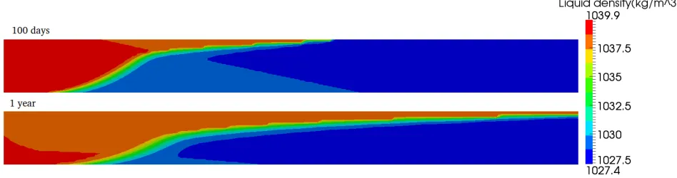
g , • the maximal liquid densityρmax
Figure 9. Liquid density evolution at a point placed 200 m away from the injection well and 25 m below the top of the aquifer. Red line represents obtained results. Blue line represents M. W. Saaltink’s results.
Figure 10. Comparison of precipitated/dissolved calcite volume fraction after 100 days of CO2 injection as a function of the time step.
The Richardson extrapolation framework [7, 22] is used to compute the convergence rates and extrapolated values of these parameters computed on three meshes with step size h1, h2 and h3, such that two consecutive
ratio are equal to two. The convergence rate p and the extrapolated valuefext are given by the well known formulas:
p= log
f3−f2 f2−f1
log
h2 h1
, fext=
f2−f1
h2 h1
p
1− h
2 h1
p . (17)
Space step size 10 5 2.5 Extrapolation Value Order
Pmax
g (MPa) 17.628 16.988 16.678 16.387 1.046
Pmax
l (MPa) 17.549 16.909 16.599 16.307 1.045 ,ρmax
g (kg.m−3) 679.23 664.26 656.41 647.75 0.931
ρmaxl (kg.m−3) 1039.2 1038.8 1038.6 1038.4 0.925
Table 5. Convergence rates and extrapolated values for characteristic flow parameters, after 100 days of injection.
Figure 11. Comparasion of precipitated/dissolved calcite volume fraction after 100 days of CO2 injection for differents meshes.
Figure 11 compares the precipitation/dissolution of calcite after 100 days of injection of CO2for three different meshes corresponding to the results exhibited in table 5. The oscillations seen of the finest mesh cannot be seen on the coarsest mesh. Their origin is actually due to the time step, but their amplitude depends on the spatial mesh size.
Finally, we note that, for the two-phase two-component flow subsystem, the Newton solver takes an average of 10 iterations. In the reactive transport subsystem, the sequential iterative algorithm takes an average of 7 iterations with a tolerance equal to 10−7.
Conclusion
CO2storage situations. This will require the development of a parallel implementation of the method (DuMuX itself already runs in parallel, but the difficulty comes from devising a load balancing strategy that would be valid both for flow and for chemistry).
Acknowledgement This work was carried out as part of the PhD thesis of V. V. The thesis was supervised by Brahim Amaziane. The authors thank Prof. Amaziane for his support and his useful advice.
References
[1] ChemEqLib: a chemical equilibrium library. webpage: https://gforge.inria.fr/projects/chemeqlib.
[2] DuMux, DUNE for multi-Phase, Component, Scale, Physics, ... flow and transport in porous media. web-page: http://www.dumux.org.
[3] DUNE, the distributed and unified numerics environment. web-page:http://www.dune-project.org.
[4] L. Amir and M. Kern. A global method for coupling transport with chemistry in heterogeneous porous media.Computational Geosciences, 14:465–481, 2009.
[5] J-B. Apoung, P. Hav´e, J. Houot, M. Kern, and A. Semin. Reactive transport in porous media.ESAIM: Proc., 28:227–245, 2009.
[6] C. M. Betke.Geochemical reaction modeling. Concepts and applications.Oxford University Press, 1996.
[7] C. Brezinksi and M. Redivo Zaglia.Extrapolation Methods. Theory and Practice.Amsterdam, North-Holland Albuquerque, 1991.
[8] J. Carrayrou, J. Hoffmann, P. Knabner, S. Kr¨autle, C. de Dieuleveult, J. Erhel, J. Van der Lee, V. Lagneau, K.U. Mayer, and K.T.B MacQuarrie. Comparison of numerical methods for simulating strongly nonlinear and heterogeneous reactive transport problems - the MoMaS benchmark case.Computational Geosciences, 14(3):483–502, 2010.
[9] J. Carrayrou, M. Kern, and P. Knabner. Reactive transport benchmark of MoMaS.Computational Geosciences, 14(3):385–392, 2010.
[10] J. Carrayrou, R. Mos´e, and P. Behra. Operator-splitting procedures for reactive transport and comparison of mass balance errors.J. Contam. Hydrol, 68:239–268, 2004.
[11] C. de Dieuleveult, J. Erhel, and M. Kern. A global strategy for solving reactive transport equations. J. Comput. Phys, 228:6395–6410, 2009.
[12] Y. Fan, L.J. Durlofsky, and H.A. Tchelepi. A fully-coupled flow-reactive-transport formulation based on element conservation, with application to CO2 storage simulations.Advances in Water Resources, 42:47–61, 2012.
[13] B. Flemisch, M. Darcis, K. Erbertseder, B. Faigle, A. Lauser, K. Mosthaf, S. Muthing S., P. Nuske, A. Tatomir, M. Wolf, and R. Helmig. DuMuX: Dune for multi-{Phase, Component, Scale, Physics, ...}flow and transport in porous media.Advances in
Water Resources, 34(9):1102–1112, 2011.
[14] G. E. Hammond, A. Valocchi, and P. Lichtner. Application of Jacobian-free Newton-Krylov with physics-based preconditioning to biogeochemical transport.Advances in Water Resources, 28:359–378, 2005.
[15] G.E. Hammond, P.C. Lichtner, C. Lu, and R.T. Mills. PFLOTRAN: Reactive flow & transport code for use on laptops to leadership-class supercomputers, pages 141–159. In Zhang et al. [31], 2012.
[16] Y. Hao, Y. Sun, and J.J. Nitao.Overview of NUFT: A versatile numerical model for simulating flow and reactive transport in porous media, pages 212–239. In Zhang et al. [31], 2012.
[17] R. Helmig.Multiphase Flow and Transport Processes in the Subsurface: A Contribution to the Modeling of Hydrosystems. Springer, 1997.
[18] X. Jiang. A review of physical modelling and numerical simulation of long-term geological storage of CO2.Applied energy, 88:3557–3566, 2011.
[19] S. Kr¨autle and P. Knabner. A reduction scheme for coupled multicomponent transport-reaction problems in porous media: Generalization to problems with heterogeneous equilibrium reactions.Water Resources Research, 43, 2007.
[20] F.M.M. Morel and J.G. Hering.Principles and Applications of Aquatic Chemistry. Wiley, New York, 1993.
[21] Intergovernmental Panel on Climate Change (IPCC). IPCC special report on carbon dioxide capture and storage. In B. Metz, O. Davidson, H.C. de Coninck, M. Loos, and L.A. Meyer, editors,IPCC Special Report on Carbon Dioxide Capture and Storage. Cambridge University Press, 2005. Prepared by Working Group III of the Intergovernmental Panel on Climate Change. [22] P.J. Roache.Verification and validation in computational science and engineering. Albuquerque: Hermosa Publishers, 1998. [23] M. Saaltink, C. Ayora, and J. Carrera. A mathematical formulation for reactive transport that eliminates mineral
concentra-tions.Water Resources Research, 34:1649–1656, 1998.
[24] M. Saaltink, F. Batlle, C. Ayora, J. Carrera, and J. Olivella. Retraso, a code for modeling reactive transport in saturated and unsaturated porous media.Geologica Acta, 2, 2004.
[26] R. Span and W. Wagner. A new equation of state for carbon dioxide covering the fluid region from the triple-point temperature to 1100 K at pressures up to 800 MPa.J. Phys. Chem. Data, 1996.
[27] M.F. Wheeler, S. Sun, and S.G. Thomas.Modeling of flow and reactive transport in IPARS, pages 42–73. In Zhang et al. [31], 2012.
[28] T. Xu and K. Pruess. Coupled modeling of non-isothermal multi-phase flow, solute transport and reactive chemistry in porous and fractured media: 1. model development and validation.Journal of Geophysical Research, 1998.
[29] T. Xu, E. Sonnenthal, N. Spycher, G. Zhang, L. Zheng, and K. Pruess. Toughreact: A simulation program for subsurface reactive chemical transport under non-isothermal multiphase flow conditions, pages 74–95. In Zhang et al. [31], 2012. [30] G.T. Yeh and V.S. Tripathi. A critical evaluation of recent developments in hydrogeochemical transport models of reactive
multi-chemical components.Water Resources Research, 25:93–108, 1989.
![Figure 1 in [25]). For convenience, we have reproduced this illustration in Figure 2.](https://thumb-us.123doks.com/thumbv2/123dok_us/10065013.1992867/10.612.143.418.158.214/figure-convenience-reproduced-illustration-figure.webp)