R E S E A R C H
Open Access
Optimal control problem governed by a
linear hyperbolic integro-differential
equation and its finite element analysis
Wanfang Shen
1*, Danping Yang
2and Wenbin Liu
3*Correspondence:
[email protected] 1School of Mathematic and
Quantitative Economics, Shandong University of Finance and Economics, Jinan, 250014, China Full list of author information is available at the end of the article
Abstract
In this paper, the mathematical formulation for a quadratic optimal control problem governed by a linear hyperbolic integro-differential equation is established. We first show the existence and regularity for the solution of the optimal control problem. The finite element approximation is based on the optimality conditions, which are also derived. Then thea priorierror estimates for its finite element approximation are obtained with the optimal convergence order. Furthermore some numerical tests are presented to verify the theoretical results.
Keywords: optimal control problem; linear hyperbolic integro-differential equations; optimality conditions; finite element methods;a priorierror estimate
1 Introduction
The distributed optimal control problem has been a classic research topic in the discipline of applied mathematics. Since it is normally difficult to obtain a closed form solution, fi-nite element approximations of optimal control problems governed by partial differential equations have been extensively studied in the literature. In particular, there have been extensive studies in convergence anda priorierror estimates of the standard finite ele-ment approximation of optimal control problems; see for instance, [–], although it is impossible to give even a very brief review here.
For optimal control problems governed by classic linear PDEs such as elliptic, parabolic and hyperbolic equations, the existence and the optimality conditions are well known, see
[]. Furthermore their finite element approximation anda priorierror estimates were
established long ago, for example, see [–, ]. Recently research has been carried out for the control governed by the integro-differential equations such as elliptic and parabolic integro-differential equations; see [, ]. However, there exists little research on the op-timal control problem governed by hyperbolic integro-differential equations, in spite of the fact that such control problems are widely encountered in practical engineering ap-plications and scientific computations. Integro-differential equations and their control of this nature appear in applications such as heat conduction in materials with memory, pop-ulation dynamics, and visco-elasticity;cf.,e.g., [–]. The physical backgrounds and the existence and uniqueness of the solution of the hyperbolic integro-differential equations have been studied in [–]. One very important characteristic of all these models is that
they all express conservation of a certain quantity; mass, momentum, heatetc.in any mo-ment for any subdomain.
Furthermore the finite element approximation of optimal control problem governed by hyperbolic integro-differential equations has not been studied yet, although there ex-ists much research on the finite element approximation of hyperbolic integro-differential equations, see,e.g.[, ].
The purpose of this paper is to investigate the weak formulation of the optimal con-trol problem governed by integro-differential equations of hyperbolic type, and then its finite element approximation. Furthermore we derive the optimality conditions and es-tablish thea priorierror estimates for the constrained optimal control problems. Finally we present some numerical tests to verify the theoretical results.
The outline of the paper is as follows. In Section , we present the weak formulation and prove the existence of the solution for the optimal control problem. In Section , we present the optimality conditions and the finite element approximation. In Section , we establish the optimala priorierror estimates for the finite element approximation of the control problem. Finally, we present some numerical tests, which illustrate the theoretical results.
2 Model problem and its weak formulation
Let, with the Lipschitz boundary∂, andUbe bounded open sets inRd, ≤d≤,
andT> . We introduce some Sobolev spaces. Throughout the paper, we adopt the
stan-dard notation Wm,q() for Sobolev spaces on with norm ·
m,q,, and semi-norm
| · |m,q,. Set W m,q
() ={w∈Wm,q() :w|∂ = }. Also denote Wm,()(Wm,()) by
Hm() (Hm
()), with norm · m,, and semi-norm| · |m,. Denote byLs(,T;Wm,q()) the Banach space of all Ls integrable functions from (,T) into Wm,q() with norm
vLs(,T;Wm,q())= (T
vsWm,q()dt)
s for s∈[,∞) and the standard modification for
s=∞. Similarly, one can define the spacesH(,T;Wm,q()) andCk(,T;Wm,q()). The details can be found in []. In addition,corCdenotes a general positive constant inde-pendent of the unknowns and the mesh parameters introduced later.
To fix ideas, we will take the state spaceW=L(,T;V) withV=H
() and the control
spaceX=L(,T;U) withU=L(U). Let the observation space beY=L(,T;H) with
H=L(). LetU
ad⊆Xbe a convex subset.
We investigate the following optimal control problem governed by a hyperbolic integro-differential equation:
min
u∈Uad⊂X
Ju,y(u)=
T
g(y) +h(u)dt (.)
subject to
⎧ ⎪ ⎨ ⎪ ⎩
ytt+Ay+
t
C(t,τ)y(τ)dτ=f +Bu, in×(,T],
y= , on∂×[,T],
y|t==y, yt|t==y, in,
(.)
where uis the control,yis the state,Uad is a closed convex subset with the respect to the control,f,y, andy are some suitable functions to be specified later.Ais a linear
depending smoothly on the spatial variables, andC(t,τ) is an arbitrary second-order linear partial differential operator, with coefficients depending smoothly on both time and spatial variables in the closure of their respective domains;Bis a suitable continuous operator. A precise formulation of this problem is given later.
Here we assumeg(·) is a convex functional which is continuously differentiable onL(),
andh(·) is a strictly convex continuously differentiable functional onU. We further assume thath(u)−→+∞asuU→+∞and thatg(·) is bounded below. Details will be specified later.
In order to give the weak formulation of problem mentioned above and study the exis-tence and regularity of the solution, we introduce theL-inner products
(f,f) =
ff, ∀(f,f)∈H×H, (u,v)U=
U
uv, ∀(u,v)∈U×U
and the bilinear forms
a(z,w) = (Az,w),
c(t,τ;z,w) =C(t,τ)z,w, ct(t,τ;z,w) =
Ct(t,τ)z,w
,
ctt(t,τ;z,w) =Ctt(t,τ)z,w.
In the case thatf∈V,f∈V∗, the dual pair (f,f) is understood asf,fV×V∗. We shall assume the convexity conditions
h(u) –h(v),u–v≥cu–v,U, ∀u,v∈L
(U), (.)
that is to say,h(·) is uniformly convex. Noting thatg(·) is convex, it is easy to see that
g(u) –g(v),u–v≥, ∀u,v∈H(). (.)
Also, we have
(Bv,w)≤cv,Uw,, ∀v∈L
(
U),u∈H(), (.)
becauseBis a bounded linear operator.
Then a possible weak formulation for the state equation reads
(ytt,w) +a(y,w) +
t
c(t,τ;y(τ),w)dτ= (f+Bu,w), ∀w∈V,t∈(,T],
y|t==y, yt|t==y.
(.)
From [–], we know that the above weak formulation has at least one solution iny∈
S(,T) ={y:y∈L(,T;H
()),yt∈L(,T;L()),ytt∈L(,T;H–())}. Therefore the control problem (.)-(.) can be restated as (OCP):
min
u∈Uad
subject to
(ytt,w) +a(y,w) +tc(t,τ;y(τ),w)dτ= (f+Bu,w), ∀w∈V,t∈(,T],
y|t==y, yt|t==y.
(.)
Next, we will analyze the existence, uniqueness, and regularity of the solution of (.). Assume that there are constantsc> andC> , such that for alltandτ in [,T]:
(a) a(z,z)≥cz,, ∀z∈V,
(b) a(z,w)≤Cz,w,, ∀z,w∈V, (c) c(t,τ;z,w)≤Cz,w,, ∀z,w∈V, (d) ct(t,τ;z,w)≤Cz,w,, ∀z,w∈V, (e) ctt(t,τ;z,w)≤Cz,w,, ∀z,w∈V.
(.)
In the following, we will give the existence and uniqueness of the solution of the system (.).
Theorem . Assume that the above conditions (a)-(d) hold. There exists a unique solution (u,y) for the minimization problem (.) such that u∈ L(,T;L(U)), y∈ L∞(,T;H
()),yt∈L∞(,T;L()),ytt∈L(,T;H–()).
Proof Let{(un,yn)}∞
n= be a minimization sequence for the system (.), then it is clear
that{un}∞
n=are bounded inL(,T;L(U)). Thus there is a subsequence of{un}∞n=(still
denoted by{un}∞
n=) such thatunconverges tou∗weakly inL(,T;L(U)). For the
sub-sequenceun, we have
yntt,w+ayn,w+
t
ct,τ;yn(τ),w(t)dτ=f+Bun,w,
∀w∈V,t∈(,T]. (.)
Takingw=yn
t in (.), we have
d dty
n t
,+a
yn,yn
=f+Bun,ynt– d
dt
t
ct,τ;yn(τ),yn(t)dτ
+ct,t;yn(t),yn(t)+
t
ct
t,τ;yn(τ),yn(t)dτ, t∈(,T]. (.)
Integrating time from totin (.), we obtain
y n t
,+
c
y n
,≤ y
,+
c
y
,+
t
f +Bun,yntdτ+εyn,
+C
t
yn,dτ+C
t
τ
From (.) and the Gronwall lemmas, we have
yn
,≤C
y,+y,+
t
f+Bun,yntdτ
+C
t
τ
yn(s),ds dτ. (.)
So we get
yn,+
t
yn,dτ≤C
y,+y,+
t
f +Bun,yntdτ
+C
t
yn(τ),+
τ
yn(s),ds
dτ, (.)
such that
yn,≤C
y,+y,+
t
f +Bun,yntdτ
. (.)
Then by (.) and (.)
ynt,≤C
y,+y,+
t
f +Bun,yntdτ
≤Cy,+y,
+C
t
f+Bun,dτ· sup ≤τ≤t
ynt(τ),. (.)
Taking the supermaximum in (.), we obtain
yntL∞(,T;L())≤C
y,+y,+fL(,T;L())+un
L(,T;L(
U))
. (.)
Then from (.) and (.), we also have
ynL∞(,T;H())≤C
y,+y,+fL(,T;L())+un
L(,T;L(U))
. (.)
Then we haveun∈L(,T;L(
U)),yn∈L∞(,T;H()) andynt ∈L∞(,T;L()). Thus
⎧ ⎪ ⎪ ⎪ ⎪ ⎪ ⎪ ⎨ ⎪ ⎪ ⎪ ⎪ ⎪ ⎪ ⎩
un−→u∈L(,T;L(
U)),
yn−→y∈L∞(,T;H()),
yn(T)−→y(T)∈H(),
yn
t −→yt∈L∞(,T;L()),
yn
t(T)−→yt(T)∈L().
Integrating time from toTin (.), we obtain
ynt(T),w(T)–y,w()
–
T
ynt,wt
dt+
T
ayn,wdt
+
T
t
ct,τ;yn(τ),wdτdt=
T
Taking the limits in (.) asn→ ∞, we have
yt(T),w(T)–y,w()
–
T
(yt,wt)dt+
T
a(y,w)dt
+
T
t
ct,τ;y(τ),wdτdt=
T
(f +Bu,w)dt,
and
T
(ytt,w)dt+
T
a(y,w)dt+
T
t
ct,τ;y(τ),w(t)dτdt
=
T
(f +Bu,w)dt, ∀w∈W. (.)
So we have
(ytt,w) +a(y,w) +
t
ct,τ;y(τ),wdτ= (f+Bu,w), ∀w∈W. (.)
Further, from (.), we obtain
yttL(,T;H–())= sup
w∈L(,T;H ())
T
(ytt,w)dt wL(,T;H
())
≤Cy,+y,+fL(,T;L())+uL(,T;L(
U))
.
This meansytt∈L(,T;H–()).
Sinceg(·) is a convex function on spaceL(,T;L()) andh(·) is a strictly convex
func-tion onU, we have
T
g(y) +h(u)dt≤ lim
n→∞
T
gyn+hundt.
So (u,y) is one solution of (.). SinceJ(u,y(u)) is a strictly convex function onUad, hence
the solution of the minimization problem (.) is unique.
The following theorem states the regularity of the solution of (.).
Theorem . Assume that the above condition(a)-(e)holds andAis an H-regularity
elliptic operator of second order and f,ft,u,ut∈C(,T;L(U)),y∈H()∩H().Then
the solution of(.)is regular in the sense that y∈L∞(,T;H
())∩L(,T;H()),yt∈
L∞(,T;H()),ytt∈L∞(,T;L()).
Proof Differentiating (.) with respect tot, we have
⎧ ⎪ ⎨ ⎪ ⎩
yttt+Ayt+C(t,t)y+
t
Ct(t,τ)y(τ)dτ=ft+But, (x,t)∈×(,T],
y= , (x,t)∈∂×[,T],
y|t==y, yt|t==y, x∈,
and we obtain
(yttt,w) +a(yt,w) +c(t,t;y,w) +
t
ct
t,τ;y(τ),wdτ= (ft+But,w). (.)
Takingw=yttin (.), we have
d dt
ytt,+a(yt,yt)
= (ft+But,ytt) –
d
dtc(t,t;y,yt) +ct(t,t;y,yt)
+c(t,t;yt,yt) – d
dt
t
ct
t,τ;y(τ),yt
dτ+ct(t,t;y,yt)
+
t
ctt
t,τ;y(τ),yt
dτ. (.)
Integrating time from totin (.), in the same way as getting (.) and (.), we can deduce
yttL∞(,T;L())+ytL∞(,T;H())
≤Cy,+y,+Ay,+fL(,T;L())
+ftL(,T;L())+uL(,T;L(U))+utL(,T;L(U))
.
Thenyt∈L∞(,T;H()) andytt∈L∞(,T;L()). Further we have
AyL(,T;L())
≤CyttL(,T;L())+fL(,T;L())+uL(,T;L(
U))+CyL(,T;L())
.
Thus by the Gronwall lemmas, y∈L(,T;H()). This completes the proof of
Theo-rem ..
Remark . In this paper, we suppose thatAis independent oft. The above results also hold for the caseA=A(x,t) provided suitable smoothness of the operatorAis assumed.
3 The optimality conditions and its finite element approximation
In this section, we study the optimality conditions and the finite element approximation for the optimal control problem governed by hyperbolic integro-differential equation.
For simplicity, we will only consider the case of quadratic objective functionals as fol-lows:
J(u,y) =
T
g(y) +h(u)dt=
T
y–zd,dt+
α
T
u,
Udt
.
Here
g(y) =
T
and
h(u) =α
T
u,Udt, (.)
wherezdis the observation.
3.1 The optimality conditions of model problem
The following theorem states the optimality conditions of the problem (.).
Theorem . A pair(y,u)∈S(,T)×X is the solution of the optimal control problem
(.),if and only there exists a co-state p∈S(,T),such that the triple(y,p,u)satisfies the following optimality conditions:
(ytt,w) +a(y,w) +tc(t,τ;y(τ),w)dτ= (f+Bu,w), ∀w∈V,t∈(,T],
y|t==y, yt|t==y;
(.)
(q,ptt) +a(q,p) +tTc(τ,t;q,p(τ))dτ= (y–zd,q), ∀q∈V,t∈[,T),
p|t=T= , pt|t=T= ;
(.)
T
αu+B∗p,v–uUdt≥, ∀v∈Uad, (.)
where B:L(
U)→L()is independent with t.B∗is the adjoint operator of B.
Proof LetJ(u,y) =g(y(u)) +j(u), where
gy(u)=
T
y–zd,dt, j(u) =
α
T
u,Udt.
By the standard method in [], the optimal conditions read
j(u)(v–u) +gy(u)(v–u)≥, ∀v∈Uad, (.)
where
j(u)(v–u)
= lim
s→+
s
ju+s(v–u)–j(u)
= lim
s→+
s
α
T
u+s(v–u), U–u
,U
dt
=
T
(αu,v–u)Udt, (.)
gy(u)(v–u)
= lim
s→+
s
gyu+s(v–u)–gy(u)
= lim
s→+
s
T
yu+s(v–u)–zd,–y(u) –zd,
= lim
s→+
s
T
y
u+s(v–u)–y(u),+ yu+s(v–u)–y(u),y–zd
dt
=
T
y(u)(v–u),y–zd
dt. (.)
Next, we computey(u)(v–u). Let us differentiate the state equation (.) atuin the directionv. By (.), we have
s
T
ytt(u+sv) –ytt(u),wdt+
T
ay(u+sv) –y(u),wdt
+
T
t
ct,τ;y(u+sv)(τ) –y(u)(τ),wdτdt
=
T
(Bv,w)dt. (.)
Taking the limits in (.) ass→, we obtain
T
y(u)(v)tt,wdt+
T
ay(u)(v),wdt+
T
t
ct,τ;y(u)(v)(τ),wdτdt
=
T
(Bv,w)dt, ∀v∈Uad,w∈W, (.)
where we used the equality that for anyz,w∈L(,T;H()), T
t
ct,τ;z(τ),w(t)dτdt=
T
T
τ
ct,τ;z(τ),w(t)dt dτ. (.)
Then (.) is equivalent to
T
y(u)(v)tt,wdt+
T
ay(u)(v),wdt
+
T
T
t
cτ,t;y(u)(v)(t),w(τ)dτdt
=
T
(Bv,w)dt, ∀v∈Uad,w∈W. (.)
Define the co-statep∈S(,T) satisfying
⎧ ⎪ ⎨ ⎪ ⎩
T
[(qtt,p) +a(q,p) + T
t c(τ,t;q(t),p(τ))dτ]dt =T(y–zd,q)dt, ∀q∈W,
p(x,T) = , pt(x,T) = .
(.)
Sincep∈S(,T), (.) is equivalent to
⎧ ⎪ ⎨ ⎪ ⎩
T
[(q,ptt) +a(q,p) + T
t c(τ,t;q(t),p(τ))dτ]dt =T(y–zd,q)dt, ∀q∈W,
p(x,T) = , pt(x,T) = .
Lettingw=pin (.), we have
T
B(v–u),pdt=
T
v–u,B∗pUdt
=
T
y(u)(v–u),ptt
+ay(u)(v–u),p
+
T
t
cτ,t;y(u)(v–u)(t),p(τ)dτ
dt
=
T
y–zd,y(u)(v–u)dt, ∀v∈Uad. (.)
By (.) and (.), we have
gy(u)(v–u) =
T
y(u)(v–u),y–zd
dt
=
T
v–u,B∗pUdt, ∀v∈Uad. (.)
By (.)-(.), and (.), the optimality conditions read
J(u)(v–u) =
T
αu+B∗p,v–uUdt≥, ∀v∈Uad, (.)
wherepis defined in (.). This completes the proof of Theorem ..
3.2 Finite element approximation
In the following, we discuss the finite element approximation of the control problem (.). Here we only consider triangular and conforming elements.
Lethbe a polygonal approximation towith boundary∂h. LetThbe a partitioning
ofhinto disjoint regularn-simplicesτ, so that¯h=
τ∈Thτ¯. Each element has at most one face on∂h, andτ¯ andτ¯have either only one common vertex or a whole edge or face ifτ¯andτ¯∈Th. We further require thatP
i∈∂h⇒Pi∈∂wherePi(i= , . . . ,J) is the vertex set associated with the triangulationTh. As usual,hdenotes the diameter of the triangulationTh. For simplicity, we assume thatis a convex polygon so that=h. Associated withThis a finite-dimensional subspaceShofC(¯h), such thatχ|τare poly-nomials of orderm(m≥) for allχ∈Sh andτ ∈Th. LetVh={v
h∈Sh:vh(Pi) = (i= , . . . ,J)},Wh=L(,T;Vh). It is easy to see thatVh⊂V,Wh⊂W.
Let Th
U be a partitioning of hU into disjoint regular n-simplices τU, so that ¯hU =
τU∈TUhτ¯U.τ¯U andτ¯
U have either only one common vertex or a whole edge or face if
¯
τUandτ¯U ∈TUh. We further require thatPi∈∂hU⇒Pi∈∂U wherePi(i= , . . . ,J) is the vertex set associated with the triangulationTh
U. For simplicity, we again assume that
Uis a convex polygon so thatU=hU. Associated withTh
Uis another finite-dimensional subspaceUhofL(hU), such thatχ|τU are polynomials of orderm(m≥) for allχ∈Uhandτ
the control. LetP() denote all the zeroth-order polynomial over. Therefore we always
takeXh={u∈X:u(x,t)|
x∈τU∈P(τU),∀t∈[,T]}.U h
ad is a closed convex set inXh. For ease of exposition, in this paper we assume thatUadh ⊂(Uad∩Xh).
Then the finite element approximation of (OCP) is thus defined by (OCP)h:
min
uh∈Uadh
T
yh–zd,dt+
α
T
uh,Udt
(.)
such that
⎧ ⎪ ⎨ ⎪ ⎩
(∂∂tyh,wh) +a(yh,wh) + t
c(t,τ;yh(τ),wh)dτ
= (f+Buh,wh), ∀wh∈Vh,t∈(,T],
yh|t==yh,
∂
∂tyh|t==yh,
(.)
whereyh∈Wh,yh∈Vh, andyh∈Vhare the approximations ofyandy.
Since (.) is a linear functional equation, and (.) is a strictly convex and finite di-mensional optimal problem, we can prove that the problem (.)-(.) has a unique so-lution (yh,uh)∈Wh×Uadh in the same way as proving the uniqueness of the solution of (.)-(.).
It is well known that a pair (yh,uh)∈Wh×Uadh is a solution of (.)-(.), if and only there exists a co-stateph∈Whsuch that the triple (yh,ph,uh) satisfies the following opti-mality conditions:
(∂∂tyh,wh) +a(yh,wh) + t
c(t,τ;yh(τ),wh)dτ = (f +Buh,wh), ∀wh∈V
h,
yh|t==yh,
∂
∂tyh|t==yh;
(.)
(qh, ∂
∂tph) +a(qh,ph) + T
t c(τ,t;qh,ph(τ))dτ= (yh–zd,qh), ∀qh∈Vh,
ph|t=T= , ∂∂tph|t=T= ;
(.)
T
αuh+B∗ph,vh–uh
Udt≥, ∀vh∈U h
ad. (.)
The optimality conditions in (.)-(.) are the semi-discrete approximation to the problem (.)-(.). LetπhUbe the local averaging operator given by
(πhUw)|τU:=
τUw
τU
, ∀τU∈TUh. (.)
It is an obvious fact that Uw=
UπhUwfor anyw∈L
(U). By the operatorπ
hU, (.)
is equivalent to
T
αuh+πhU
B∗ph
,vh–uh
Udt≥, ∀vh∈U h
ad. (.)
4 A priorierror analysis
For simplicity, we consider the zero obstacle problem:
Uad=
v∈X;v≥, a.e.x∈U,t∈[,T], (.)
or the integration obstacle problem:
Uad=
v∈X;
U
v≥,t∈[,T]
. (.)
In the case of (.), (.) and (.) yield
(y,p,u)∈L,T;H()×L,T;H()×L,T;H(U)
. (.)
In the case of (.), (.) and (.) yield
(y,p,u)∈L,T;H()×L,T;H()×L,T;H(U). (.) In the following, we will give thea priorierror estimates inL∞(,T;H())-norm. We
first present some lemmas.
Lemma . Let Uadbe given by(.)or(.).ThenπhUw∈Uadh for any w∈Uad. Let us introduce the auxiliary problem
⎧ ⎪ ⎨ ⎪ ⎩
(∂
∂tyh(u),wh) +a(yh(u),wh) +
t
c(t,τ;yh(u)(τ),wh)dτ = (f+Bu,wh), ∀wh∈Vh,
yh(u)|t==yh,
∂
∂tyh(u)|t==y h
;
(.)
⎧ ⎪ ⎨ ⎪ ⎩
(qh,∂∂tph(u)) +a(qh,ph(u)) +
T
t c(τ,t;qh,ph(u)(τ))dτ = (y–zd,qh), ∀qh∈Vh,
ph(u)|t=T= , ∂∂tph(u)|t=T= .
(.)
Since (yh(u),ph(u)) is the standard finite element of (y,p), from [], we get the following results.
Lemma . Let(yh(u),ph(u))be the solutions of the systems(.)-(.).Then we have the a priori error estimates
y–yh(u)L∞(,T;H())+
∂∂ty–yh(u)
L∞(,T;L())
+p–ph(u)L∞(,T;H())+
∂∂tp–ph(u)
L∞(,T;L())≤
Ch, (.)
y–yh(u)L(,T;L())+p–ph(u)L(,T;L())≤Ch. (.)
yh–yh(u)L∞(,T;H())+
∂∂tyh–yh(u)
L∞(,T;L())
+ph–ph(u)L∞(,T;H())
+∂
∂t
ph–ph(u)
L∞(,T;L())
+u–uhL(,T;L(
U))≤C
hU+h
. (.)
Proof From (.) and (.), we obtain
⎧ ⎪ ⎨ ⎪ ⎩
(∂∂t(yh–yh(u)),wh) +a(yh–yh(u),wh) +
t
c(t,τ; (yh–yh(u))(τ),wh)dτ
= (B(uh–u),wh), ∀wh∈Vh,
(yh–yh(u))|t== , ∂∂t(yh–yh(u))|t== .
(.)
Similarly, from (.) and (.), we have
⎧ ⎪ ⎨ ⎪ ⎩
(qh, ∂
∂t(ph–ph(u))) +a(qh,ph–ph(u)) +
T
t c(τ,t;qh, (ph–ph(u))(τ))dτ = (yh–y,qh), ∀qh∈Vh,
(ph–ph(u))|t=T= , ∂∂t(ph–ph(u))|t=T= .
(.)
Takingwh=∂∂t(yh–yh(u)) in (.), we obtain
d
dtyh–yh(u)
t
,+a
yh–yh(u),yh–yh(u)
=B(uh–u),
yh–yh(u)
t – d dt t
ct,τ;yh–yh(u)
(τ),yh–yh(u)
dτ+ct,t;yh–yh(u),yh–yh(u)
+ t ct
t,τ;yh–yh(u)
(τ),yh–yh(u)
dτ. (.)
Integrating time from totin (.) and noting that (yh–yh(u))|t== ,∂∂t(yh–yh(u))|t== , we have
∂∂tyh–yh(u)
,
+yh–yh(u),
≤C
t
uh–u,Udτ+C
t
∂∂tyh–yh(u)
,
dτ+εyh–yh(u),
+C
t
yh–yh(u),dτ+C
t
τ
yh–yh(u)
(s),ds dτ. (.)
Lettingεbe small enough, we get
∂
∂t
yh–yh(u)
,
+yh–yh(u)
,+
t
yh–yh(u) ,dτ
≤C
t
uh–u,Udτ+C
t ∂ ∂t
yh–yh(u)
,
+yh–yh(u)
,
+
τ
yh–yh(u)
(s),ds
By the Gronwall lemma, we have
∂
∂t
yh–yh(u)
L∞(,T;L())
+yh–yh(u)L∞(,T;H())
≤Cuh–uL(,T;L(U)). (.)
Similarly lettingqh=∂∂t(ph–ph(u)) in (.), we also have
∂
∂t
ph–ph(u)
L∞(,T;L())
+ph–ph(u)L∞(,T;H()) ≤Cyh–yL(,T;L())
≤Cy–yh(u)L(,T;L())+Cu–uhL(,T;L(
U)). (.)
From (.), (.), and Lemma ., we only need to estimateu–uhL(,T;L(
U)). Since
u–uhL(,T;L(U))≤ u–πhUuL(,T;L(U))+πhUu–uhL(,T;L(U)),
we need the estimateπhUu–uhL(,T;L(
U)). From (.), (.), we have
απhUu–uh
L(,T;L(
U))
=α T
(u,u–uh)U+ (uh,uh–πhUu)U+ (u,πhUu–u)U
dt ≤ T
B∗p,uh–u
U+
B∗ph,πhUu–uh
U+α(u,πhUu–u)U
dt = T
B∗(p–ph),uh–πhUu
U+
B∗p+αu,πhUu–u
U
dt. (.)
On the one hand, we takewh=ph–ph(u) in (.), andqh=yh–yh(u) in (.), and inte-grate time from toT, to have
T
B(uh–u),ph–ph(u)
–yh–y,yh–yh(u)
dt = ∂ ∂t
yh–yh(u)
,ph–ph(u)
t=T
t=–
yh–yh(u),
∂ ∂t
ph–ph(u) t=T t= + T t
ct,τ;yh–yh(u)
(τ),ph–ph(u)
(t)dτdt
–
T
T
t
cτ,t;yh–yh(u)
(t),ph–ph(u)
(τ)dτdt= .
Then
T
uh–πhUu,B
∗(p–p
h) Udt = T
uh–πhUu,B
∗p–ph(u)
Udt+
T
yh(u) –yh,yh–y
+
T
πhUu–u,B
∗p
h–ph(u)
Udt
≤ T
uh–πhUu,B
∗p–ph(u)
Udt+
T
yh(u) –yh,yh(u) –ydt
+
T
πhUu–u,B
∗p
h–ph(u)
Udt
≤Cy–yh(u)
L(,T;L())+p–ph(u)
L(,T;L())+hUu–πhUu
L(,T;L(
U))
+εuh–πhUu
L(,T;L(
U))+yh–yh(u)
L(,T;L())
+ph–ph(u)
L(,T;H())
≤Ch+hUu–πhUu
L(,T;L(
U))
+εuh–πhUu
L(,T;L(
U)) +yh–yh(u)
L(,T;L())+ph–ph(u)
L(,T;H())
. (.)
On the other hand
B∗p+αu,πhUu–u
U≤CB
∗p–π
hU
B∗p,
U+u–πhUu
,U
. (.)
Applying the above two estimates, from Lemma ., we can get
πhUu–uhL(,T;L(
U))≤C
hU+h
. (.)
Thus we complete the proof of Lemma ..
Then from Lemma ., Lemma ., and the triangle inequality, we have the following.
Theorem . Let(y,p,u)and(yh,ph,uh)be the solutions of the systems(.)-(.)and (.)-(.).Then we have the a priori error estimate:
y–yhL∞(,T;H())+
∂∂t(y–yh)
L∞(,T;L())
+p–phL∞(,T;H())
+∂
∂t(p–ph)
L∞(,T;L())
+u–uhL(,T;L(
U))≤C(hU+h). (.)
5 Numerical experiment
In this section, we carry out a numerical experiment to verify thea priorierror estimates derived in Section . The numerical tests were done by using AFEpack software package (see []).
In the numerical example, we take=U= [, ]. We use linear finite element spaces to approximate the state and co-state, and the piecewise constant finite element spaces to approximate the control. For the time variable, a Euler backward-difference procedure is used to solve the discrete system. Here the time step size is controlled to demonstrate the relation between the error function and the spatial sizes.
The numerical example is the following control problem:
min
u≥
(y–zd)+
u
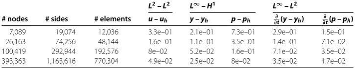
Table 1 Numerical result: for adaptive time steps 50
L2–L2 L∞–H1 L∞–L2
# nodes # sides # elements u–uh y–yh p–ph ∂t∂(y–yh) ∂t∂(p–ph)
7,089 19,074 12,036 3.3e–01 2.1e–01 7.3e–01 2.9e–01 1.5e–01
26,163 74,256 48,144 1.6e–01 1.1e–01 3.5e–01 1.4e–01 7.1e–02
100,419 292,944 192,576 8e–02 5.2e–02 1.6e–01 7.1e–02 3.5e–02
393,363 1,163,616 770,304 4.9e–02 2.5e–02 8e–02 3.5e–02 1.7e–02
subject to
ytt– y–
t
(t–τ) y dτ=f +u, x∈, <t< ,
y|∂= .
(.)
The solutions of (.)-(.) are
⎧ ⎪ ⎪ ⎪ ⎪ ⎪ ⎪ ⎨ ⎪ ⎪ ⎪ ⎪ ⎪ ⎪ ⎩
p= –(T–t)sinπx
sinπx, T= ,
u=max{–p, },
y=tx
( –x)x( –x),
zd=y–ptt+ p+
T
t (t–τ) p dτ,
f =ytt– y–
t
(t–τ) y dτ–u.
(.)
The numerical results are put in Table . In Table , the errors inL∞(,T;H()) (L–
L)-norm,L∞(,T;H()) (L–H)-norm andL∞(,T;L()) (L∞–L)-norm are listed. From Table , we see that theL-norm convergent rate of the control variableu–uh isO(h),i.e., we have first-order accuracy with respect to the spatial size; theH-norm convergent rate of the state and co-state variables y–yh andp–ph also areO(h); and theL-norm convergent rate of the state and co-state approximation errors ∂
∂t(y–yh) and ∂
∂t(p–ph) areO(h), consistent with our theoretical analysis. 6 Conclusions
In this paper, a quadratic optimal control problem governed by a linear hyperbolic integro-differential equation and its finite element approximation are investigated for the first time. By selecting suitable state and control spaces, and defining the bilinear forms, the
mathematical formulation is established. Thena prioriestimates have been carried out
using the standard functional analysis techniques, and the existence and regularity of the solution are provided by using these estimates. We then approximate the optimal control using the standard finite element method and study the approximation errors. Based on these studies,a priorierror estimates with the optimal convergence rates are derived. Fi-nally numerical results are presented. Through our investigation, it is clear the standard finite element method works well, both from the point of view of theory and practice, for the quadratic optimal control governed by a linear hyperbolic integro-differential equation when there is no convection term present. However, when there exists strong convection, it is very likely that very different finite element approximation schemes need to be used.
Competing interests
The authors declare that they have no competing interests.
Authors’ contributions
Author details
1School of Mathematic and Quantitative Economics, Shandong University of Finance and Economics, Jinan, 250014,
China.2Department of Mathematics, East China Normal University, Shanghai, 200241, China.3KBS, University of Kent, Kantebury, CT27NF, England.
Acknowledgements
The authors express their thanks to the referees for their valuable comments and suggestions. This work is supported by National Natural Science Foundation of China (Grant: 11326226), Science and Technology Development Planning Project of Shandong Province (No. 2012G0022206) and Nature Science Foundation of Shandong Province (No. ZR2012GM018).
Received: 2 April 2014 Accepted: 27 June 2014 References
1. Alt, W: On the approximation of infinite optimisation problems with an application to optimal control problems. Appl. Math. Optim.12, 15-27 (1984)
2. Falk, FS: Approximation of a class of optimal control problems with order of convergence estimates. J. Math. Anal. Appl.44, 28-47 (1973)
3. French, DA, King, JT: Approximation of an elliptic control problem by the finite element method. Numer. Funct. Anal. Optim.12, 299-315 (1991)
4. Malanowski, K: Convergence of approximations vs. regularity of solutions for convex, control constrained, optimal control systems. Appl. Math. Optim.8, 69-95 (1982)
5. Neittaanmäki, P, Tiba, D: Optimal Control of Nonlinear Parabolic Systems: Theory, Algorithms and Applications. Dekker, New York (1994)
6. Pironneau, O: Optimal Shape Design for Elliptic Systems. Springer, Berlin (1984)
7. Tiba, D: Lectures on the Optimal Control of Elliptic Equations. University of Jyväskylä Press, Jyväskylä (1995) 8. Tiba, D: Optimal Control of Nonsmooth Distributed Parameter Systems. Springer, Berlin (1990)
9. Tiba, D, Tröltzsch, F: Error estimates for the discretization of state constrained convex control problems. Numer. Funct. Anal. Optim.17, 1005-1028 (1996)
10. Lions, JL: Optimal Control of Systems Governed by Partial Differential Equations. Springer, Berlin (1971) 11. Hermann, B, Yan, NN: Finite element methods for optimal control problems governed by integral equations and
integro-differential equations. Numer. Math.101, 1-27 (2005)
12. Shen, W, Ge, L, Yang, D: Finite element methods for optimal control problems governed by linear quasi-parabolic integro-differential equations. Int. J. Numer. Anal. Model.10, 536-550 (2013)
13. Millor, RK: An integro-differential equation for rigid heat conductions with memory. J. Math. Anal. Appl.66, 313-332 (1978)
14. London, S, Staffans, O: Volterra Equations. Lecture Notes in Math., vol. 737. Springer, Berlin (1979) 15. Staffans, O: On a nonlinear hyperbolic Volterra equation. SIAM J. Math. Anal.11, 793-812 (1980)
16. Dafermos, C, Nohel, J: Energy methods for nonlinear hyperbolic Volterra integro-differential equations. Commun. Partial Differ. Equ.41, 219-278 (1979)
17. Ismatov, M: A mixed problem for the equation describing sound propagation in a viscous gas. J. Differ. Equ.20, 1023-1035 (1984)
18. Sun, P: The finite element methods and application of interpolated techniques for hyperbolic integro-differential equations. Math. Appl.9, 433-440 (1996)
19. Zhang, T, Li, C: Superconvergence of finite element approximations to parabolic and hyperbolic integro-differential equations. Northeast. Math. J.17(3), 279-288 (2001)
20. Lions, JL, Magenes, E: Non Homogeneous Boundary Value Problems and Applications. Die Grundlehren der mathematischen Wissenschaften, Band 181. Springer, Berlin (1972)
21. Liu, WB, Yan, NN: Adaptive Finite Elements Methods for Optimal Control Problem Governed by PDEs. Sciences Press, Beijing (2008)
22. Li, R: On multi-meshh-adaptive algorithm. J. Sci. Comput.24, 321-341 (2005) doi:10.1186/s13661-014-0173-8