Scholarly Horizons: University of Minnesota, Morris
Undergraduate Journal
Volume 5 | Issue 2
Article 1
June 2018
Querying Large Databases
Nathan Beneke
University of Minnesota, Morris
Follow this and additional works at:
https://digitalcommons.morris.umn.edu/horizons
Part of the
Databases and Information Systems Commons
This Article is brought to you for free and open access by the Journals at University of Minnesota Morris Digital Well. It has been accepted for inclusion in Scholarly Horizons: University of Minnesota, Morris Undergraduate Journal by an authorized editor of University of Minnesota Morris Digital Well. For more information, please [email protected].
Recommended Citation
Beneke, Nathan (2018) "Querying Large Databases,"Scholarly Horizons: University of Minnesota, Morris Undergraduate Journal: Vol. 5 : Iss. 2 , Article 1.
Cover Page Footnote
This work is licensed under the Creative Commons Attribution- NonCommercial-ShareAlike 4.0
Querying Large Databases
Nathan Beneke
Division of Science and Mathematics University of Minnesota, Morris Morris, Minnesota, USA 56267
[email protected]
ABSTRACT
This paper investigates two approaches to improving query times on large relational databases. The first technique cap-italizes on the knowledge of a database’s structures and properties one typically has. This technique can execute some queries exactly in a constant, bounded amount of time. When this technique cannot be used to exactly execute a query we show how it can still be used to drastically lower the run-time on the query while getting a good approxi-mation of the exact result. We also discuss the complexity of deciding whether a query is evaluable in this way, both theoretically and practically. The second approach approx-imates aggregate queries by incorporating only part of the data, rather than all of the data the query pertains to. We briefly investigate an established method of sampling a ran-dom subset of the data, and then a newer method which par-tially reads every tuple and puts deterministic error bounds on the results.
Keywords
Big Data, Relational Database, Approximate Query Pro-cessing, Scale Independent Queries
1.
INTRODUCTION
All around us, we hear that we are living in the world of “big data.” What challenges does the world of big data bring? In the modern world, we all rely on vast databases to quickly and accurately retrieve our data for us in many areas. As datasets grow in size, querying these datasets quickly be-comes cost-prohibitive. There is a trade-off between hard-ware cost and time it takes to complete a query, and even if we assume an infinite budget for hardware, modern tech-nology has its limits. A linear search through a dataset–a search which takes a linear amount of time relative to how large the dataset is–that’s a petabyte in size would take days with a modern solid state drive [3]. It’s this challenge that this paper addresses: how does one query a large database in a reasonable amount of time given limited resources?
The need for efficient methods to query large databases is evident, and techniques can be split into two categories: those that execute queries exactly, and those that only ap-proximate queries. These techniques, while powerful, have
This work is licensed under the Creative Commons Attribution-NonCommercial-ShareAlike 4.0 International License. To view a copy of this license, visit http://creativecommons.org/licenses/by-nc-sa/4.0/.
UMM CSci Senior Seminar Conference, April 2018Morris, MN.
their own limitations and drawbacks. They don’t always work in the general case of all queries for all databases. When a technique is universally applicable, it isn’t always ideal for all data distributions or all types of queries. All techniques are subject to properties of the database, such as structure and data distribution, or even the data type. When approximating a query, it is not always possible to guarantee error bounds before it is made, and they often require a lot of precomputation [2].
It’s also important to note the difference between a database and a dataset. While a dataset is simply a set where each element is a single data point, it is not structured like a rela-tional database. A database is a way of structuring datasets in a more useful way. For this paper, when we talk about a dataset we assume that it can be represented by a relational database.
In this paper, we define terms and notations for relational databases, as well as for specific methods discussed in the paper, in section 2; discuss a method that can evaluate some queries exactly in constant time, and how the same method can be used to approximate other queries in constant time in section 3; give an overview of an iterative algorithm that can approximate aggregate queries with arbitrary precision in section 4; and conclude in section 5.
2.
RELATIONAL DATABASES
This section addresses concepts, definitions, and notations necessary to understanding relational databases that is rel-evant in all sections.
A relational database consists of tables, also called rela-tions, in which each row, ortuple, contains one entry in the database. Two tuples in the same table will always be com-prised of the same attributes, corresponding to columns in the table.
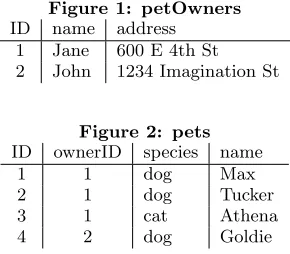
Two tables can relate to each other by referencing an-other table’sprimary key, a set of columns that can be used to uniquely identify any row in the table. In all of the ex-amples in this paper the primary key is a single column, titled ID, that has the express purpose of being a unique number that can be used as a key, however there is no rea-son it has to be only one column [6]. For example consider a database that aims to store data about people and their pets. This database consists of just two tables, a petOwners ta-ble with attributes{ID, name, address}, and apetstable with attributes {ID, ownerID, species, name}. In these tables IDis the primary key for each respective table, and is guaranteed to be unique within that table, whileownerID is aforeign keythat references thepetOwnerstable. These
1
Beneke: Querying Large Databases
Figure 1: petOwners
ID name address 1 Jane 600 E 4th St 2 John 1234 Imagination St
Figure 2: pets
ID ownerID species name 1 1 dog Max 2 1 dog Tucker 3 1 cat Athena 4 2 dog Goldie
tables represent aone-to-many relationship, as one person may have many pets, but each pet may only have 1 owner. See figures 1 and 2 for some example entries in this database. A query, informally, is a question about the data in a database. More formally, a query is a function that maps from a database to a set of tuples, whose fields are dependent on the query itself, matching certain constraints [6]. For ex-ample, one could query the example database above as such: "what are the names of all dogs and their correspond-ing owners’ names". The query would then return a set of tuples with fields{dogName, ownerName}, with one tuple for each dog in thepetstable, as in figure 4 shown below. For the purpose of this paper we will assume that queries do not alter any data.
The result of a query involving multiple tables is a subset of thecartesian product of those tables. A cartesian prod-uct of two tables lists every possible combination of tuples in those two tables, and most entries are meaningless, slowing down searches considerably. See figure 3 for the cartesian product of figures 1 and 2. In figure 3 only those tuples wherepetOwners.ID=pets.ownerIDare meaningful, and it also still lists cats even though we are only interested in dogs for our query. The relation formed by taking the cartesian product of two or more tables is ajoin. For large databases joins present a problem because if table 1 con-tains n tuples and table 2 contains m tuples, then their cartesian product containsn∗m tuples. Asn and m can grow to be quite large in practical applications, this can eas-ily become unmanageable. This difficulty can be even more difficult in practice as many queries are performed on more than two tables.
Anindexis a copy of specific fields in a database as a data structure that allows for lookups faster than a linear search through a table. Typically these fields are in the same table, although they do not have to be. Some indexes can even be functions mapping tuples in one table to tuples in another table. Indexes are usually mapped to actual memory or disk locations as well, and are used to decrease query times. This is aided by the use of data-structures that can be searched inO(log(n)) or sometimes evenO(1) time, such as binary trees and hash-maps.[6] For example, if there is an index on the names of pet owners stored as a hash table, then we would be able to query the database for pet owners with specific names in constant time, rather than linear time, with respect to the number of pet owners. You can also use indexes to avoid searching through the cartesian product of two tables for queries involving joins. As another example, if there were an index on petOwners.ID to pets.name and pets.species, we could look up the names of any individual’s
pets using this index rather than by doing a linear search through the cartesian product pictured in figure 3.
3.
SCALE INDEPENDENT QUERIES
3.1
Notation
Because some tables have fields with identical names we use a dot notation to distinguish them. We write [ta-ble].[field]to denote a specific field in a specific table. TheIDfield in thepetOwnerstable ispetOwners.IDand is distinct frompets.ID. To avoid spacial clutter, we only use this notation when it is necessary for clarity.
In this section, we use a notation similar to functional notation to describe queries: Q(D) would denote the results of query Q on the datasetD. Note thatD andQ(D) are considered as sets, whileQis mathematically thought of as a relation from some space of possible tuples to a different space of tuples.
We also assume that a subset of any dataset, when rep-resented as a relational database, shares the same structure as the original set in terms of what tables it is comprised of and what fields those tables are comprised of.
We also use a notation to describe relationships between tables. For example, if there is nobody who owns more than 20 pets we could write the relationship between the pet owners table and the pets table as R({petOwners.ID} → {petOwners.name, address},20). If somebody adopted a 21st pet we could writeR({petOwners.ID} →
{petOwners.name, address},21). R(X →Y, N) denotes a relationship between a set,X, of fields in a database, to the set of fields,Y, where this is a one to many relationship with one tuple of fieldsXrelated to at mostN tuples of fieldsY. Note thatN is a property of the specific set of data, while
X andY are properties of any relational database with the same architecture. This allows us to put a bound on re-lationships between tuples in different tables, so that for a simple query it is easy to put a bound on how many results there are. With the second relationship we know the query ”what are the names of all the pets belonging to a partic-ular person” would have at most 21 results. We call these relationshipsaccess constraints and the entire set of access constraints that apply to a database anaccess schema.
3.2
Boundedly Evaluable Queries
We call a query Q scale independent in a dataset D if
Q(D) can be executed with the same amount of work, re-gardless of how largeD is. More formally,Qis scale inde-pendent inD if there exists anM ≥0 such that:
1. M is independent of|D|.
2. There exists a D0 ⊆ D such that |D0| ≤ M and
Q(D0) =Q(D).
This ensures that if you can identify D0 you only have to
search through at mostM tuples to executeQ(D). [3] A queryQis said to beboundedly evaluableinDwith re-spect to an access schemaAifQ(D) can be evaluated using only the access constraints inAand it is scale independent. Note that we can be sureQ(D) is scale independent when using only access constraints in Ato be executed if all re-lationships in Ahave a finiteN. We use Ato identifyD0
Figure 3: Cartesian Product of petOwners and pets
petOwners.ID petOwners.name petOwners.address pets.ID pets.ownerID pets.species pets.name
1 Jane 600 E 4th St 1 1 dog Max
1 Jane 600 E 4th St 2 1 dog Tucker
1 Jane 600 E 4th St 3 1 cat Athena
1 Jane 600 E 4th St 4 2 dog Goldie
2 John 1234 Imagination St 1 1 dog Max 2 John 1234 Imagination St 2 1 dog Tucker 2 John 1234 Imagination St 3 1 cat Athena 2 John 1234 Imagination St 4 2 dog Goldie
Figure 4: Pets and Owners
dogName ownerName Rex Jane Tucker Jane Goldie John
For example, consider the same database as in previous examples, now with an additional table,petNicknames, con-sisting of columns{ID, petID, nickname}, listing nicknames for the pets wherepets.ID=petNicknames.petID. We call this databaseD. LetQ be the following query: Find the nicknames of all dogs Jane owns. IfD satisfies the fol-lowing access constraints, thenQis boundedly evaluable in
D. The access constraints are:1
(a) R({petOwners.name} → {petOwners.ID},5)
(b) R({petOwners.ID} → {pets.ID, species, pets.name},20) (c) R({pets.ID} → {petN icknames.ID, nickname},7)
Then if there are indexes matching these constraintsQcan be evaluated onD by accessing only 5∗20∗7 = 700 tuples and in constant time. Otherwise there would need to be a linear search through the cartesian product of the three tables, accessing n∗m∗p tuples, where n is the number of tuples in the petOwners table and m is the number of tuples in thepetstable andpis the number of tuples in the petNicknamestable.
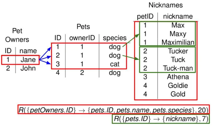
In order to do the lookup in constant time one uses con-straint (a) to find up to five IDs for pet owners namedJane, in this case finding onlypetOwners.ID= 2, then use that and access constraint (b) to find at most 20 IDs for the pets, and finally use access constraint (c) to match those pets to their nicknames (see figure 5 for a diagram). Now that we have all the petsJane owns, we can filter that list to only be dogs. Evaluating the query in this way accesses at most 700 tuples, and what’s more, no matter how many pet owners and pets are inD, this number will remain 700. The tuples the execution accesses comprise D0 ⊆ D and
M = 700 ≥ |D0|in this case, making Qscale independent
inD.
Not all queries are boundedly evaluable, even when they have similar structure to queries known to be boundedly evaluable. For example, ”Find all owners’ names and pair them with all the nicknames of their dogs” is not boundedly
1Note that the numbers could be any finite positive integers,
these were chosen arbitrarily, and that this is just one ex-ample of a set of access constraints that makesQboundedly evaluable inD.
evaluable under the given access constraints. This is because you can’t start with any specific owners’ names like you can in the previous example. In order to use the indexes built with the access constraints, you would first have to iterate over the names of all pet owners, which is linear with regard to the number of tuples in the petOwners table. So if we were to insert another pet owner into the table, the number of tuples we access would increase. Thus this query is not scale independent or boundedly evaluable.
Not all queries are boundedly evaluable and further, it is undecidable in the general case whether a given query is boundedly evaluable. However, there are important classes of queries where this problem is decidable. This is expanded on in section 3.5.
Note that for any scale independent queryQinD there exists some access schema with whichQis boundedly evalu-able. Any boundedly evaluable query is also scale indepen-dent. However, the definitions are still significantly different as scale independence is a general desirable property of a query which is very difficult to practically draw conclusions about, while with bounded evaluability we can achieve scale independence through indexes hinted at by the definition.
3.3
Boundedly Evaluable Envelopes
When a queryQis not boundedly evaluable in a dataset
Dit is still desirable to reduce the amount of work needed to evaluate it. It is often possible to find boundedly evaluable queries Ql and Qu such that Ql(D) ⊆ Q(D) ⊆ Qu(D).
Ql(D) andQu(D) arelower and upper envelopes of Q(D),
respectively. We can also find constants Nl and Nu such
that |Q(D)−Ql(D)| ≤ Nland |Qu(D)−Q(D)| ≤ Nu, we
call theseapproximation boundsforQlandQuwith respect
toQ.
Informally, we return a set that is too small, and a set that is too large. We then search through the set difference to obtain the exact result of the query.
Not all queries have upper and lower envelopes, and in general it is undecidable whether a query has an upper en-velope. This is expanded on in section 3.5
3.4
An Implementation of Bounded
Evalua-bility
BEAS (Bounded Evaluation of SQL) [1] is a demonstra-tion of the feasibility of bounded evaluability, written as a database management system for PostgreSQL 9.4.6 and tested with an anonymous telecommunications company on datasets up to 200GB in size.
The architecture of BEAS consists of three modules: AS Catalog, BE Query Planner, and BE Plan Executor. AS Catalog is the module responsible for maintaining the
3
Beneke: Querying Large Databases
Figure 5: A flow diagram of an evaluation plan for a boundedly evaluable query. Here the tuples outlined in red compriseD0.
indexes, metadata, and access schema. It also automati-cally discovers a set of access constraints from the database’s contents and structure and then builds hash indexes of those constraints. BE Query Planner checks whether queries are boundedly evaluable in the given dataset and access schema, then constructs an evaluation plan for all queries. If a query is boundedly evaluable, it constructs a plan utilizing that, otherwise it identifies sub-queries that are boundedly evalu-able and uses indexes from the access constraints to optimize a conventional query plan. BE Plan Executor executes these plans through the use of thefetchoperator, which uses the indexes to fetch values in constant time rather than through joins. Because a boundedly evaluable query has an upper bound on the amount of data accessed in its evaluation, BEAS allows the user to inquire whether it is possible to evaluate a query with a given limit on resources, without actually executing the query.
The database BEAS was tested on has 12 relations with 285 total fields, obtained and used by an anonymous telecom-munications company. BEAS took 0.1, 0.4, 0.7, 0.9, and 1.1 seconds on the same query in datasets the size of 1, 10, 50, 100, and 200 gigabytes respectively. This was com-pared to conventional Database Management Systems with the same query, the fastest was PostgreSQL which took 8.8, 91.5, 459.7, 933.6, and 1932.5 seconds on the same datasets respectively. With this testing data the scalability and ef-fectiveness of BEAS and bounded evaluation in general is clearly shown.
3.5
Decidability and Complexity
In general, the question of whether a queryQis boundedly evaluable or scale independent on any dataset that conforms to a set of access constraints,A, is undecidable2. In
prac-tice, however, we typically only need to know whetherQis boundedly evaluable in a specific dataset,D. This second
2i.e. There is no possible algorithm which can answer this
question for all cases in a finite amount of time.
question is still NP-complete3, however. Fortunately, the practical problem is even more specific, that is whetherQis scale independent inD with respect to a boundM. When
M is specified, the complexity is still NP-complete for all queries.
Although it would be nice for this problem to be decid-able in general, or even in polynomial time for a givenM, there are still desirable cases which can be computed effi-ciently. Conjunctive queries are queries that are built from simple atomic logical statements such as x =y or x≤ y. These atomsare connected with logical conjunction(s) and existential quantifiers. This class of queries covers most non-aggregate queries that one might ask of a database and are much easier to investigate the scale independence of. Al-though it is still undecidable whether a conjunctive query is scale-independent in any dataset that conforms toA, and NP-complete for any specificD, it is in polynomial time with regards to a specificM.
There are also many other classes of queries and common cases where it is in polynomial time to decide whether the query is boundedly evaluable. In fact, for most practical applications this problem is in polynomial time. [4]
4.
APPROXIMATE AGGREGATE QUERIES
Often the goal of a query is not to produce a list of some tuples. An aggregate value is based on multiple tuples such as average, sum, or maximum of a given field. With our example of pets and pet owners, one might query “find the average age of the pets for every pet owner.” Queries like these are known asaggregate queries.
The results of aggregate queries are not always needed ex-actly, and so it is desirable to approximate them when possi-ble. For example, if you wanted to know the average income
3
of people in a city, you probably wouldn’t need the exact figure, only an estimation with narrow error-bounds. First, in subsection 4.1 there will be a brief overview of sampling-based aggregate querying (SAQ), and its limitations. Then, in subsection 4.2 we will describe a newer approach called deterministic approximate querying.
4.1
SAQ - The Established Approach
Sampling-based Approximate Querying (SAQ) is approxi-mating a query by performing it on a random subset of the dataset. This typically works well for some aggregate func-tions, such as average, but fails to accurately approximate other functions such as maximum, which are very sensitive to extremes.
All aggregate functions, including average, are somewhat sensitive to outliers. Outliers are unlikely to be in a small random sample of data, and using a large subset reduces efficiency gains for this method. Thus if our dataset has an extreme outlier estimates of aggregate functions on that data are unlikely to be very accurate. Some aggregate func-tions are more sensitive to outliers than others. For example maximum is very affected by outliers, while average is less affected by outliers. We could, for instance, survey 5% of a city’s population to approximate the income distribution of the entire city. If we took the average of this sample, it would probably be very close to the true average. However, if we took the maximum income of our sample, it would probably not be very close to the actual maximum income in the city.
Compounding this issue is that confidence intervals are difficult to determine exactly, and even to approximate them-selves. This is especially true for the functions that are already difficult to accurately estimate with SAQ such as maximum. SAQ can also make it difficult to reason about confidence intervals. If you seek the average of some field, and get a result with 95% confidence, this tells you nothing about the distribution in the tails. [5]
4.2
DAQ - A Deterministic Approach
Deterministic approximate Querying(DAQ) is an approach to query approximation that deterministically evaluates the upper and lower bounds of its estimates. When using DAQ, one can choose a number of iterations to apply the scheme. Each iteration of a DAQ scheme makes the estimate more accurate, and there is a finite number of iterations such that the estimate is the exact result of the query and the upper bound equals the lower bound [5]. DAQ can be implemented in different ways. We will specifically cover a bitwise DAQ scheme.
In abitwise DAQ scheme, to evaluate a query for a given field, we evaluate the nth most significant bit of the field for each tuple in thenthiteration. For example, to find the maximum of an 8-bit field, on the first iteration you would only look at the most significant bit for each tuple. Suppose there is at least one tuple where the most significant bit is a 1. Then the maximum of the field is at least 27, and at most 28−1. Then if we do another iteration, only looking at
tuples already known to have the most significant bit 1, we look at the second bit and no tuples have a 1, but at least one tuple has a 0. Now we know the maximum for the field is at least 27, but is not larger than 27+ 26.
Notice in the above example our error decreased exponen-tially in the 2nd iteration, and will continue to do so every
Figure 6: How a column is indexed using bitslices. [5]
iteration until the exact answer is obtained. Additionally, by performing bitwise comparisons, we are able to ignore a certain number of bits, and for aggregation functions based on comparison–such as maximum, it is often possible to ob-tain the exact answer before examining all of the bits if the tuple containing the maximum is identified before doing so. It is also worth noting here that in this scheme, the error bounds function mathematically as rounding errors, rather than statistical uncertainty.
This method is not as suitable for all aggregation func-tions, however. In a table withN tuples, and while we are ignoringbbits, the error for maximum is 2b−1 while for a
function such as sum that error must be taken into account for every tuple and thus the error is N∗(2b−1). When averaging with bitwise DAQ, it is also impossible to obtain the exact answer before examining all of the bits unlike with maximum.
In order to make this approach computationally benefi-cial, the use of abitsliced index is necessary. Each field in the database that we wish to be able to use bitwise DAQ on is indexed with an array of bitslices (also called bitvec-tors). The first bitslice contains the most significant bit of every row in the table, the second bitslice contains the sec-ond most significant, and so on. See figure 6 for a graphical representation of this data structure. Then in order to per-form an iteration of any aggregate function using bitwise DAQ we simply use the array of bitslices for that bit and perform the necessary bitwise operations. Building these in-dexes is very expensive, in terms of computation time, so it should be decided upon in advance what fields they will be necessary for and then constantly maintained rather than building the index as part of the query. It would also be possible to use a similar index scheme but slice by bytes, or some other delimiter, but this has yet to be explored. [5]
4.3
DAQ compared to SAQ and to Exact
Eval-uation
How well bitwise DAQ does compared to SAQ and to an exact typical evaluation scheme depends on the data dis-tribution and the aggregation function these methods are used on. There are distributions and functions that SAQ is clearly superior to DAQ, and vice versa.
On a uniform data distribution, taking a 5% random sam-ple to compute the average of a field, SAQ yields a 1% error, and is about 20 times faster than an exact evaluation. Using bitwise DAQ is only 5 times faster than an exact evaluation when yielding a 1% error. However when applied to the function “top 100”, which asks for the 100 largest values in the table, DAQ easily outperforms SAQ on uniform
distri-5
Beneke: Querying Large Databases
butions. On a Zipf4 distribution with parameter s = 1.5
distribution, SAQ requires nearly 100% sampling to accu-rately approximate top 100, while bitwise DAQ needs only the first 6 bits of 32 bit unsigned integers to achieve 1% accuracy, while being about 4 times faster than an exact evaluation. In the experiment DAQ even converged to the exact answer after examining only the most significant 12 bits. [5]
A method of compressing the bitslice index was also im-plemented, which improved performance times considerably. Bitslicing also lends itself easily to parallelization, as you can divide up the columns into ranges, each range to be pro-cessed in a different thread, and then collate the data once all threads are finished. This requires very little overhead as in most cases almost no shared data is required.
These experiments indicate that, while DAQ is not about to revolutionize data processing, in many circumstances it outperforms the established SAQ. If an exact answer isn’t required, DAQ in all test cases outperformed the baseline of a traditional evaluation. [5]
5.
CONCLUSION
There is still a lot of room for improvement in evaluating queries quickly, both exactly and approximately. Although a lot of promising work has been done, including real-life implementation and use in the case of bounded queries, all approaches have their limitations.
Boundedly evaluable queries work very well when they can be used, however it is undecidable in general to know whether a query is boundedly evaluable, and many impor-tant sub-classes of queries and sub-problems remain NP-complete. The authors (W. Fan and others) have inves-tigated the decidability and complexity of many other re-lated problems and classes of queries as well. This approach works very well for queries that are known to be bound-edly evaluable and need to be executed frequently, as well as most conjunctive queries. The main limitation remains that there are queries which are not boundedly evaluable at all, although the same researchers are working on another approach making use of the same data properties called in-cremental scale independence. This technique is most useful for queries which are computationally expensive but per-formed often. Informally, it is simply precomputingQ(D) once, and then updating that result on demand by access-ing at mostM tuples. Incremental scale independence was implemented in BEAS as a method to optimize queries that are not scale independent, and is worth further investigation as well.
Approximating aggregate queries via SAQ works well for functions that are not sensitive to outliers such as aver-age, and on distributions that don’t have very many out-liers, such as uniform and normal distributions. However on other distributions that do have a lot of outlier and on func-tions that are sensitive to outliers, such as maximum, DAQ
4
The Zipf distribution is a very tail-heavy distribution, typ-ically used to model data such as the populations of cities or the word frequencies of a spoken language ranked by most used to least used. When represented on a graph with both axes on a log scale, the Zipf distribution appears approx-imately linear. Having a higher parameter indicates that more sample points are greater than the mean. In the fol-lowing examples about 77% of sample points are greater than the mean. [5]
is a promising new approach. Although DAQ rarely offers the same performance gain that SAQ does, it allows users greater control over their error bounds, and lends itself more easily to algebraic manipulation. Bitwise DAQ specifically works well for numeric data, and it would be interesting to see the results of DAQ being applied to other types of data, such as strings. A formal algebra has also been defined for DAQ (the general approach, not specific to bitwise DAQ), that is a modification of relational algebra and accounts for the deterministic error bounds. This algebra is outside the scope of this paper, but would be an interesting topic for a different project or further investigation.
Both approaches discussed have an additional downside in that they rely on the use of indexes that are computation-ally expensive to compute, and space intensive to store. An index necessarily duplicates some data. When multiple in-dexes have to be computed or maintained on databases that are hundreds of gigabytes in size these indexes accumulate their own costs in terms of maintenance and data storage.
Acknowledgments
Thank you to Elena Machkasova, my advisor and senior seminar professor, for her extensive advice and feedback. I would also like to thank Peter Dolan for his help under-standing database concepts and Jacob Opdahl, my alumni reviewer.
6.
REFERENCES
[1] Y. Cao, W. Fan, Y. Wang, T. Yuan, Y. Li, and L. Y. Chen. Beas: Bounded evaluation of SQL queries. In
Proceedings of the 2017 ACM International Conference on Management of Data, SIGMOD ’17, pages
1667–1670, New York, NY, USA, 2017. ACM. [2] S. Chaudhuri, B. Ding, and S. Kandula. Approximate
query processing: No silver bullet. InProceedings of the 2017 ACM International Conference on Management of Data, SIGMOD ’17, pages 511–519, New York, NY, USA, 2017. ACM.
[3] W. Fan, F. Geerts, Y. Cao, T. Deng, and P. Lu. Querying big data by accessing small data. In
Proceedings of the 34th ACM
SIGMOD-SIGACT-SIGAI Symposium on Principles of Database Systems, PODS ’15, pages 173–184, New York, NY, USA, 2015. ACM.
[4] W. Fan, F. Geerts, and L. Libkin. On scale
independence for querying big data. InProceedings of the 33rd ACM SIGMOD-SIGACT-SIGART Symposium on Principles of Database Systems, PODS ’14, pages 51–62, New York, NY, USA, 2014. ACM.
[5] N. Potti and J. M. Patel. Daq: A new paradigm for approximate query processing.Proc. VLDB Endow., 8(9):898–909, May 2015.
[6] Wikipedia. Relational database — Wikipedia, The Free Encyclopedia, 2018. [Online; accessed February-2018]. [7] Wikipedia contributors. NP-completeness —

![Figure 6: How a column is indexed using bitslices.[5]](https://thumb-us.123doks.com/thumbv2/123dok_us/8863883.1809437/7.612.322.549.56.140/figure-column-indexed-using-bitslices.webp)
