Volume 2009, Article ID 468971,21pages doi:10.1155/2009/468971
Review Article
An Overview of the Coding Standard MPEG-4 Audio
Amendments 1 and 2: HE-AAC, SSC, and HE-AAC v2
A. C. den Brinker,
1J. Breebaart,
1P. Ekstrand,
2J. Engdeg˚ard,
2F. Henn,
2K. Kj¨orling,
2W. Oomen,
3and H. Purnhagen
21Philips Research Laboratories, High Tech Campus 36, 5656 AE Eindhoven, The Netherlands
2Dolby Sweden AB, G¨avlegatan 12 A, 11330 Stockholm, Sweden
3Philips Applied Technologies Eindhoven, High Tech Campus 5, 5656 AE Eindhoven, The Netherlands
Correspondence should be addressed to A. C. den Brinker,[email protected]
Received 29 September 2008; Accepted 24 February 2009
Recommended by James Kates
In 2003 and 2004, the ISO/IEC MPEG standardization committee added two amendments to their MPEG-4 audio coding standard. These amendments concern parametric coding techniques and encompass Spectral Band Replication (SBR), Sinusoidal Coding (SSC), and Parametric Stereo (PS). In this paper, we will give an overview of the basic ideas behind these techniques and references to more detailed information. Furthermore, the results of listening tests as performed during the final stages of the MPEG-4 standardization process are presented in order to illustrate the performance of these techniques.
Copyright © 2009 A. C. den Brinker et al. This is an open access article distributed under the Creative Commons Attribution License, which permits unrestricted use, distribution, and reproduction in any medium, provided the original work is properly cited.
1. Introduction
The MPEG-2 Audio coding standard was released in 1997 and has successfully found its way into the market. Later, MPEG-4 Audio Version 1 and Version 2 were issued in mid 1999 and early 2000, respectively. These versions have adopted the MPEG-2 AAC coder including several exten-sions to it. In addition several other components like speech coders (HVXC and CELP) and a Text-To-Speech Interface are specified.
In 2001, MPEG identified two areas for improved audio coding technology and issued a Call for Proposals (CfP, [1]). These two areas were
(i) improved compression efficiency of audio signals or speech signals by means of bandwidth extension which is forward and backward compatible with existing MPEG-4 technology;
(ii) improved compression efficiency of high-quality audio signals by means of parametric coding.
This started a new cycle in the standardization process, consisting of a competitive phase leading to a selection of the reference model, a collaborative phase for improving the
technology and, finally, the definition of a new standard. Close to the finalization of the work on parametric coding, it was demonstrated that the parametric stereo (PS) module that was developed in the course of the this work item could also be combined with the bandwidth extension technology thereby providing a significant additional boost in coding efficiency. This particular combination was subsequently added to the parametric coding amendment. The work on bandwidth extension and parametric coding reached the final stage of Amendment 1 and 2 to MPEG-4 Audio mid 2003 and 2004, respectively.
This paper has the intention to outline the ingredients of the MPEG-4 Audio Amendments in a comprehensive way. Part of this material is present in the literature but mostly scattered. Therefore, this paper sets out to give an overview of the three components that make up these Amendments with references to more detailed information where necessary.
The outline of the paper is as follows. The basic technology and subjective test results for the bandwidth extension and parametric coding are discussed in Sections2
Audio input
SBR encoder
SBR data
Filtered audio
data
Core encoder
Bit mux
Bitstream
SBR data
Bit de mux
Core decoder
Audio data
SBR decoder
Audio output
Figure1: SBR incorporates pre- and postprocessing stages: SBR parameters are extracted from the input signal in the SBR encoder and transmitted together with the encoded low-band signal. The decoded low-band signal is bandwidth extended by the SBR decoder, spectrally adjusted and enhanced in accordance with the transmitted SBR data.
2. MPEG-4 SBR
2.1. Introduction. High-Frequency Reconstruction/Regen-eration (HFR), or BandWidth Extension (BWE), techniques have been researched in the speech coding community for decades [2,3]. The underlying hypothesis stipulates that it should be possible to reconstruct the higher frequencies of a signal given the corresponding low-frequency content only. In the speech coding community this research was done with the goal to be able to accurately reconstruct the high-band of a speech signal given only the low-pass filtered low-band signal and no other a priori information about the high-band of the original signal. Typically the high-band was recreated by upsampling of the low-band signal without subsequent low-pass filtering (aliasing), or by means of broad-band frequency translation (single side-band modulation) of the low-band signal [2,3]. The spectral envelope of the recreated high-band was either simply whitened and tilted with a suitable roll-offat higher frequencies, or in more elaborate versions [4] estimated by means of statistical models. This research has not led to any wide adoption of such an HFR-based speech enhancement in the market as of today.
The original SBR technique (of which the development started in early 1997) differs from previously known HFR techniques [5,6].
(i) The primary means for extending the bandwidth is transposition, which ensures that the correct harmonic structure is maintained for single- and multipitched signals alike.
(ii) Spectral envelope information is always sent from the encoder to the decoder making sure that the spectral envelope of the reconstructed high-band is correct [7].
(iii) Additional means such as inverse filtering, noise, and sinusoidal addition, guided by transmitted informa-tion, compensate for shortcomings of any bandwidth extension method originating from occasional fun-damental dissimilarities between low-band and high-band [8,9].
These features successfully enabled the use of a band-width extension technique not only for speech signals but for arbitrary signals. The fundamental topology of a system employing SBR is shown inFigure 1. An audio input signal is first processed by an SBR encoder, resulting in a low-pass filtered audio signal and SBR data. The audio signal is subsequently encoded using a core encoder. Finally, the SBR
data and the core-coder output are combined into an output bit stream. The decoder performs the reverse process.
Since the HFR method enables a reduction of the core coder bandwidth and the HFR technique requires significantly lower bit rate to code the high-frequency range than a waveform coder would, a coding gain can be achieved by reducing the bit rate allocated to the waveform core coder while maintaining full audio bandwidth. Naturally, this gives the possibility to decrease the total data rate by lowering the crossover frequency between core coder and the HFR part. However, since the audio quality of the HFR part cannot scale towards transparency, this crossover frequency is always a delicate tradeoff between core coder and HFR related artifacts.
This paper only covers SBR in the MPEG context, where it is standardized for use together with AAC, forming the (High Efficiency) HE AAC Profile. However, the algorithm and bit stream are essentially core codec agnostic, and SBR has successfully been applied to other codecs such as MPEG Layer-2 [10] and MPEG Layer-3 (the latter case is known as mp3PRO, see [11]), it is included in (High Definition Codec) HDC, that is, the proprietary codec used by iBiquity, and is standardized within (Digital Radio Mondiale) DRM for use together with the CELP and HVXC speech codecs [12]. Furthermore, it is worth noting that the transposition method included in the MPEG-4 standard is a carefully selected tradeoffbetween implementation cost and quality, relaxing the strict requirements on harmonic continuation that are met by more advanced transposition methods.
2.2. System Overview
2.2.1. SBR Encoding Process
Overview. Following the general process of MPEG to standardize transmission formats and decoder operation (and hence allowing future encoder-side improvements) the SBR amendment contains an informative (as opposed to normative) encoder description. Hence this section gives a generic overview of the various elements of an encoder; the exact design of these elements is left up to the implementer. However, for detailed information on a realization of the encoder capable of high perceptual performance, the 3GPP specification of the SBR encoder is a good source, see [13].
SBR encoder Audio
input 2fs
Down-sampling
2:1
Audio signal
fs
QMF analysis (64 bands)
Control parameter extraction
Envelope estimator Bitrate control
Control data SBR data
Core encoder
Bitstream
Uncompressed audio signal Data path
Figure2: Block scheme of the SBR encoder. The core of the system comprises a QMF bank and a spectral envelope estimator.
filter banks of the (Quadrature Mirror Filter) QMF type. The encoder has an analysis bank per input channel, and the decoder has an analysis and synthesis pair per channel. Most of the SBR processing, such as encoder-side parameter extraction and decoder-side bandwidth extension and spectral envelope adjustment, is performed in the QMF domain.
QMF Analysis. The original time-domain input signal is first filtered in a 64-channel analysis QMF bank. The filter bank splits the time-domain signal into complex-valued subband signals and is thus oversampled by a factor of two compared to a regular real-valued QMF bank [14]. For every 64 time-domain input samples, the filter bank produces 64 subband samples. At 44.1 kHz sample rate this corresponds to a nominal bandwidth of 344 Hz, and a time resolution of 1.4 ms. All the subsequent modules in the encoder operate on the complex-valued subband samples.
Transient Detection. A transient detector (part of the “Con-trol parameter extraction” in Figure 2) operates on the complex-valued subband signals in order to assist the envelope estimator in the time/frequency (T/F) grid selec-tion. Generally, longer time segments of higher frequency resolution are produced by the envelope estimator during quasistationary passages, while shorter time segments of lower frequency resolution are used for dynamic passages. The transient detection is, for example, accomplished by calculating running short-term energies and detecting signif-icant changes.
T/F Grid Selection and Envelope Estimation. The estimated envelope data are obtained by averaging of subband sample energies within segments in time and frequency. The time borders of these segments are determined mainly by the output from the transient detector, and are subsequently signaled to the decoder. When the transient detector signals a transient to the envelope estimator, segments of shorter duration in time are defined by the envelope estimator, starting with a minimal segment, the leading border of
which is placed at the onset of the transient. Subsequent to the short-time segment by the transient, somewhat longer segments are used to correctly track a potential decay of the transient, and finally long segments are used for the stationary part of the signal.
The main objective is to avoid pre- and postechoes that otherwise would be induced by the envelope adjustment process in the decoder for transient input signals.
The envelope estimator also decides on the frequency resolution to use within each time segment. The variable frequency resolution is achieved by employing two different schemes for grouping of QMF samples in frequency: high resolution and low resolution, where the number of estimates differs by a factor of two. In order to reduce instantaneous peaks in the SBR bit rate, the envelope estimator typically trades one high-resolution envelope for two low resolution ones. The grouping in frequency can be either linearly spaced or (approximately) log spaced where the number of bands to use per octave is variable. An example of a T/F grid selection is given in Figure 3 where the grid is superimposed on a spectrogram of the input signal. As is clear from the figure, the time resolution is higher around the transient events, albeit with lower frequency resolution, and vice versa for the more stationary parts of the signal.
Although the segment borders can be chosen with a high degree of freedom, the temporal resolution, as well as the frequency resolution, is constrained by the analysis QMF bank resolution. The filter bank is designed to provide a resolution in both time and frequency that is considered adequate for the adjustment of the envelope for all signal types. Hence the filter bank resolution is not adaptive, as is usually the case for filter banks in perceptual waveform coders, and the estimates are achieved by, within a filter bank of fixed size, adaptively grouping and averaging of subband sample energies as outlined above.
regeneration of the high-band. This is done in an analysis-by-synthesis fashion. In Figure 4such an analysis-by-synthesis process is illustrated. In the top panel of the figure a spectrum of the input signal is given. In this particular example the input signal is a synthetically generated test signal of which the tonal (harmonic) structure ends abruptly above 5.5 kHz. The remaining spectrum of the signal consists of noise. In the lower panel of the figure a spectrum is given of the high-band given the HF generation method used in the decoder,withoutadditional correction of tonal-to-noise properties. In this case, the tonal structure of the low-band has propagated to the high-band (the region from 5.5 kHz to 15 kHz) and hence within the region of 5.5 to 15 kHz, there is a mismatch in signal characteristics between original input and reconstructed high-band signal. The transmission of additional noise information allows correction of such mismatches. It should be noted that the spectrum in the lower panel illustrates the low-band signal in combination with the high-band signal after HF generation without any subsequent envelope adjustment.
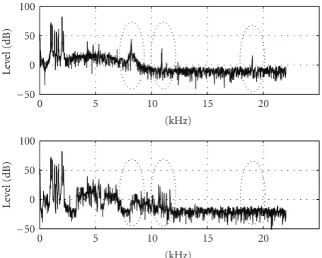
Missing Harmonics Detection. Similarly to the above sit-uation, the encoder also needs to assess whether strong tonal components in the original high-band signal will be missing after the high-frequency reconstruction. InFigure 5
an example is given where three strong tonal components are not reconstructed by the high-frequency regeneration based on the low-band signal. Again an analysis-by-synthesis approach can be beneficial. For this example a glockenspiel signal is used. In the upper panel ofFigure 5the spectrum for the input signal is given, where three strong tonal components in the high-band are indicated by circles. In the lower panel of Figure 5the spectrum of the HF-generated signal is given similarly to the example inFigure 4. Clearly the three strong tonal components will not be properly regenerated by the HF generator, and therefore need to be replaced by sinusoids generated separately in the decoder. Information on the (frequency) location of these strong tonal components is transmitted to the decoder, and the missing components are inserted in the high-band signal.
Quantization and Encoding. The SBR envelope data, tonal component data, and noise-floor data are quantized and differentially coded in either the time or frequency direction in order to minimize the bit rate. All data is entropy coded using Huffman tables. Details about SBR data coding are given in the next section.
2.2.2. SBR Bit Stream
Overview. To ensure consistent coding of transients regard-less of localization within codec frames, the SBR frames have variable time boundaries, that is, the exact duration in time covered by one SBR frame may vary from frame to frame. The bit stream is designed for maximum flexibility such that it scales well from the lowest bit rate applications up to medium and high bit rate use cases, and is easy to adapt for
0.5 0.4
0.3 0.2
0.1 0
(s) 0
5 10 15 20
(kHz)
Figure 3: T/F grid selection example. The white dashed lines illustrate the borders of the time-frequency tiles superimposed on the spectrogram of the input signal. The leading edge and decay of the transient is encoded with short low frequency resolution envelopes, and the quasistationary passages in between transients are represented by longer high-frequency resolution envelopes.
20 15
10 5
0
(kHz) −50
0 50 100
Le
ve
l
(d
B
)
20 15
10 5
0
(kHz) −50
0 50 100
Le
ve
l
(d
B
)
Figure 4: Illustration of the mismatch in noise level of the reconstructed high-band if no additional noise information is transmitted to the decoder. This can be used for an analysis-by-synthesis method in the SBR encoder in order to assess the amount of noise that should be added on the decoder side. The upper panel shows the spectrum of the (synthetically generated) input signal, and the lower panel shows a spectrum of the signal obtained after HF generation based on the low-band signal without noise correction. The SBR range covers the frequency range from 5.5 kHz to 15 kHz.
20 15
10 5
0
(kHz) −50
0 50 100
Le
ve
l
(d
B
)
20 15
10 5
0
(kHz) −50
0 50 100
Le
ve
l
(d
B
)
Figure 5: Illustration of missing sinusoidal components in the high-band (if no additional sinusoidal signals are added in the decoder). This can be used for an analysis-by-synthesis method in the SBR encoder in order to assess where a sinusoid should be added on the decoder side. The upper panel shows the spectrum of the input signal (a glockenspiel signal), and the lower panel shows a spectrum of the signal obtained after HF generation based on the low-band signal without adding separate sinusoids. The SBR range covers the frequency range from 5.5 kHz to 15 kHz.
2.2.3. SBR Decoding Process
Overview. The block scheme of the SBR decoder is given
in Figure 6. The bit stream is input to the core decoder
providing the low-band signal, and the SBR relevant bit stream to the SBR decoder. The SBR decoder performs a 32 subband analysis of the low-band signal, which is subse-quently used, along with control data from the bit stream, by the HF generator to create the high-band signal. The envelope of the recreated high-band signal is subsequently adjusted and additional signal components are added to the high-band. The combined low-band and high-band are finally synthesized by a 64 subband QMF synthesis filter bank in order to obtain the time-domain output signal. The analysis and synthesis filter banks are constructed such that an upsampling of the low-band signal by a factor of two is inherently obtained in the processing. A detailed description of the decoder can be found in the MPEG-4 Audio standard [15]. In the following, we merely outline the various decoding steps.
An example is given inFigure 7. The original input signal spectrum is shown in the top-left panel. The spectrum of a low-band output from the AAC core decoder is given in the top right panel ofFigure 7. It is clear that the signal is low-pass filtered at approximately 6 kHz which is the bandwidth covered by the core coder for the setting corresponding to the bit rate used in this example. It should be noted that in the figure the signal has been upsampled to the sampling frequency of the original signal (and also that of the final output signal) in order to allow for spectrum comparison.
The HF Generator transposes parts of the low-band frequency range to the high-band frequency range covered by SBR as indicated in the bit stream. In the bottom left panel of
Figure 7the spectrum of the transposed intermediate signal
in combination with the low-band signal is displayed. This is how the output would look if no envelope adjustment of the recreated high-band would be performed.
The envelope adjuster adjusts the spectral envelope of the recreated high-band signal according to the envelope data and time/frequency grid that was transmitted in the bit stream. Additionally, noise and sinusoid components are added as signaled in the bit stream. The output from the SBR decoder after envelope adjustment is depicted in the bottom right panel ofFigure 7. In the following the decoding steps are examined in more detail.
QMF Analysis. The time-domain audio signal, supplied by the core decoder and usually sampled at half the frequency of the original signal, is first filtered in the analysis QMF bank. The filter bank splits the time-domain signal into 32 subband signals. For every 32 time-domain samples, the filter bank produces 32 complex-valued subband samples and is thus over-sampled by a factor of two compared to a regular real-valued QMF bank. The oversampling enables significant reduction of impairments emerging from modifications of subband signals. The oversampling is accomplished through extension of a cosine modulated filter bank with an imag-inary sine modulated part, forming a complex-exponential modulated filter bank. In a conventional cosine modulated filter bank the analysis and synthesis filtershk(n) and fk(n) are cosine modulated versions of a symmetric low-pass prototype filterp0(n) as
hk(n)=2p0(n) cos
π
2M(2k+ 1)
n−N
2 − M
2
,
fk(n)=2p0(n) cos
π
2M(2k+ 1)
n−N
2 + M
2
, (1)
wherek = 0· · ·M−1,M is the number of channels and n=0· · ·N, whereNis the prototype filter order.Figure 8
depicts a simplified block scheme for the implementation of a cosine modulated filter bank. For complex modulation both filters are obtained from
hk(n)= fk(n)=p0(n) exp
π
2M(2k+ 1)
n−N
2
. (2)
The terms containingM/2 (terms needed for aliasing cancel-lation) present in the traditional cosine modulated filter bank omitted because of the complex-valued representation [14].
InFigure 9the corresponding block scheme for a
SBR decoder
Bitstream Core decoder
Audio signal
fs
SBR data
QMF analysis (32 bands)
HF generator
Envelope adjuster
Additional HF components
QMF synthesis (64 bands)
Audio output 2fs
Uncompressed audio signal Data path
Figure6: Block scheme of the SBR decoder. The received bit stream is input to the core decoder decoding the low-band audio signal, and providing the SBR decoder with the SBR relevant bit stream data. The SBR decoder performs a QMF analysis of the low-band signal which is subsequently used for the HF Generation providing a high-band signal. The high-band is envelope adjusted and additional signal components are added. Finally, the output signal is obtained by a QMF synthesis filter bank.
20 15
10 5
0
Frequency (kHz) −50
0 50
Le
ve
l
(d
B
)
Original
20 15
10 5
0
Frequency (kHz) −50
0 50
Le
ve
l
(d
B
)
AAC output
20 15
10 5
0
Frequency (kHz) −50
0 50
Le
ve
l
(d
B
)
HF generation
20 15
10 5
0
Frequency (kHz) −50
0 50
Le
ve
l
(d
B
)
aacPlus output
Analysis QMF bank
Time domain input signal (real-valued)
Polyphase filtering
Cosine modulation R
Synthesis QMF bank Cosine
modulation
Polyphase
filtering Time domain output signal (real-valued)
Figure8: Simplified block scheme of a Cosine Modulated QMF bank implementation.
Analysis QMF bank
Time domain input signal (real-valued)
Polyphase filtering
Cosine modulation
Sine modulation
R
I
j j
Synthesis QMF bank Cosine
modulation +
Polyphase filtering Sine
modulation
Time domain output signal (real-valued)
Figure9: Simplified block scheme of a Complex Exponential Modulated QMF bank implementation.
HF Generation. The complex-valued subband signals obtained from the filter bank are processed in the high-frequency generation unit to obtain a set of high-band subband signals. The generation is performed by selecting low-band subband signals, according to specific rules, which are mirrored or copied to the high-band subband channels. The patches of QMF subband to be copied, their source range and target range, are derived from information on the borders of the SBR range, as indicated by the bit stream. The algorithm generating the patch structure has the following objectives.
(i) The patches should cover the frequency range up to 16 kHz with as few patches as possible, without using the QMF subband lowest in frequency (i.e., the subband including DC) in any patch.
(ii) If several patches constitute the high-band, a patch covering a lower frequency range should have a wider or equal bandwidth compared to a patch covering a higher frequency range. The motivation is that for lower frequencies the human hearing is more sensitive, and therefore patches with wide bandwidth are preferred for lower frequencies in order to move any potential discontinuity between the first and the second patch as high up in frequency as possible.
(iii) The source frequency range for the patches should be as high up in frequency as possible.
Creating the high-band in this way has several advantages and is the reason why SBR can be referred to as a semi-, or quasi-, parametric method. Although the high-band is synthetically generated and shaped by the SBR bit-stream data, the characteristics of the high-band are inherited from the low-band, and, which is the most important aspect, so is the temporal structure of the high-band. This makes the corrections of the high-band, in order to resemble the
original, much more likely to succeed in the subsequent processing steps.
With the above in mind, the characteristics of the low-band and the high-low-band still vary for different audio signals. For example, the tonality is usually more pronounced in the low-band than in the high-band. Therefore, inverse filtering is applied to the generated high-band subband signals. The filtering is accomplished by in-band filtering of the complex-valued signals using adaptive low-order complex-complex-valued FIR filters. The filter coefficients are determined through an analysis of the low-band in combination with control signals extracted from the SBR data stream. A second-order linear predictor is used to estimate the spectral whitening filter using the covariance method. The amount of inverse filtering is controlled by a chirp-factor given from the bit stream. Hence, the HF-generated signal yk(n) for QMF subbandk and time slotnin the high-band can be defined according to
yk(n)=xl(n)−αl(0)γkxl(n−1)−αl(1)γ2kxl(n−2), (3) whereαl(0) andαl(1) are given by the prediction error filter estimated for the low-band subbandl, and whereγk is the chirp factor (between 0 and 1) controlled by the bit stream.
InFigure 10an example of patching and inverse filtering
is given. In the top panel of the figure, a (power) spectrum of the low-band signal is displayed, and the maximum source region for the patching is indicated. For all subbands within this region, prediction error filters are estimated as outlined above. The source range in the low-band is patched, in this example, to region A and B. The frequency plot of the patched signals in these regions are given in the lower panel of Figure 10. Here three inverse filtering regions are also indicated by 1, 2, and 3. The applied inverse filtering level is the same within these regions and its parameters are contained in the bit stream.
20 15
10 5
0
Frequency (kHz) −50
0 50
Le
ve
l
(d
B
)
AAC lowband signal Frequency range used for
HF patch and estimation of filter coefficients
A B
20 15
10 5
0
Frequency (kHz) −50
0 50
Le
ve
l
(d
B
)
HF Generated highband signal
1 2 3
Frequency range of first HF patch
Frequency range of second HF patch
Frequency ranges of inverse filtering bands
Figure 10: Example of high-frequency generation and inverse filtering. The figure shows the frequency spectra of the low-band signal and the subsequent high-low-band signals. The signal is an excerpt of a classical music piece coded at 24 kbps mono. The frequency range for SBR, as given in the bit stream for the configuration used, is 5.5 kHz to 15 kHz. This range is covered by two consecutive patches, A and B, where A has a larger frequency range. Finally, three inverse filtering regions are given by the bit stream, where the frequency border of the second and third region coincide with the patch border.
region. Thus, the suitable prediction error filter coefficients are available for all subbands within region A and B. Hence, for all the QMF subbands within the region 1 inFigure 10
an inverse filtering is done within each subband, given the corresponding prediction error filter estimated on the corresponding low-band subband samples and the chirp factor signaled in the bit stream for the specific region.
It should be noted that all the processing done in the HF Generation module is done frame-based on a time segment indicated by the outer borders of the SBR frame.
The generated high-band signals are subsequently fed to the envelope adjusting unit.
Envelope Adjustment. The most important, and also the largest part of the SBR data stream, is the spectrotemporal envelope representation of the high-band. This envelope representation is used to adjust the energy of the generated high-band subband signals. The envelope adjusting unit first performs an energy estimate of the high-band signals. An accurate estimate is possible because of the complex-valued subband signal representation. The resulting energy samples are subsequently averaged within segments according to control signals from the data stream. This averaging produces the estimated envelope samples. Based on the estimated envelope and the envelope representation extracted from the
data stream, the energy of the high-band subband samples in the respective segments are adjusted.
As previously outlined sinusoids present in the original high-band signal that have no corresponding sinusoid in the generated high-band are synthesized in the decoder, and random white noise is added to the high-band signal to compensate for diverging tonal-to-noise ratios of the high-band and low-high-band.
A noise floor levelQis used to derive the level of noise to be added to the recreated high-band signal, it is defined as the energy ratio between the HF-generated (by means of patching in the HF generator) signal energy and the noise signal energy of the final output signal.
Given the calculated gain values, a limiting procedure is applied. This is designed to avoid the need to excessively high-gain values due to large differences in the transposed signal energy and the reference energy given by the original input signal. The limiter is operative to limit high narrow-band gain values while ensuring that the correct wide-narrow-band energy is maintained.
QMF Synthesis. The generated high-band signals and the delay-compensated (resulting from the HF generation pro-cess) low-band signals are finally supplied to the 64-channel synthesis filter bank, which usually operates at the sampling frequency of the original signal. The synthesis filter bank is just like the analysis filter bank complex-valued, however the imaginary part of the output signal is discarded. Thus, the filter bank generates a real-valued full bandwidth output signal having twice the sampling frequency of the core coder signal.
2.2.4. Other Aspects
Low Power SBR. The SBR tool as outlined in the previous sections is defined in two versions: a High Quality Version and a Low-Power version. The main difference is that the Low-Power version utilizes real-valued QMF filter banks, while the High Quality version utilizes complex-valued filter banks. In order to make the SBR Tool work in the real-valued domain, additional tools are included that strive to minimize the introduction of aliasing in the SBR processing. The main feature is an aliasing detection algorithm that identifies adjacent QMF subbands with strong tonal components in the overlapping range. The detection is done by studying the reflection coefficient of a first-order in-band linear predictor. By observing the signs of the reflection coefficients for adjacent subbands, the subbands prone to introduce aliasing can be identified. For the identified subbands restrictions are put on how much the gain adjustment is allowed to vary between the two subbands.
The following text and figures provide an example of low-power SBR. Envelope adjustment in a real-valued QMF filter bank is displayed inFigure 11.
25 24 23 22 21 20 19 18 17 16 15
Frequency (π/M)
20 40 60 80 Le ve l (d B
) Frequency analysis of input signal
25 24 23 22 21 20 19 18 17 16 15
Frequency (π/M)
−20 0 20 Le ve l (d B
) Gain vector
25 24 23 22 21 20 19 18 17 16 15
Frequency (π/M)
20 40 60 80 Le ve l (d B
) Spectral envelope adjustment using a real valued filter bank
Figure11: Envelope adjustment in a real-valued QMF filter bank. In the top panel, sinusoids are displayed within QMF subbands. The QMF subband responses are stylistically drawn and at a higher frequency resolution than that of the filter bank, in order to illustrate where within the QMF subband the sinusoids are located. The second panel illustrates the gain vector as calculated by the envelope adjustment module, where the gain values are given for every subband. The third panel illustrates the output after envelope adjustment. Here it is evident that, for example, the sinusoid located between subbands 16 and 17, where also the gain values differ between the subbands, will produce an aliasing component that is not part of the signal in the top panel.
on every subband are displayed. As can be seen these vary from subband to subband. In the bottom panel the high-resolution frequency analysis is again displayed, albeit this time after application of the gain values. As can be observed from the figure, aliasing is introduced.
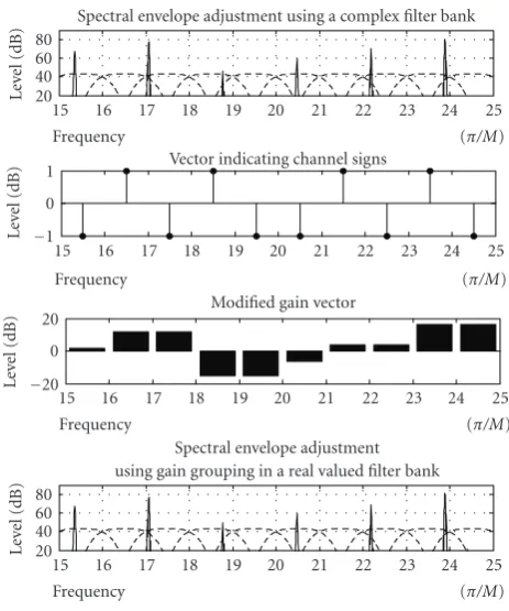
Figure 12 demonstrates aliasing detection and aliasing
reduction. This figure is very similar toFigure 11except for a new panel with “channel signs.” These signs are derived from the reflection coefficients of a first-order predictor, where
sign(x)=
⎧ ⎨ ⎩
(−1)k ifα1<0,
(−1)k+1 ifα1≥0,
(4)
and whereα1is given by the prediction error filter
A(z)=1−α1z−1 (5)
obtained by in-band linear prediction of the subband samples, andkindicates the subband (indexed from zero). Given the definition of the signs and certain relations between the signs of adjacent subbands, the reduction of aliasing can be established by modifying the gain values in the gain vector. For adjacent subbands where the lower subband (in frequency) has a positive sign, and the higher subband (in frequency) has a negative sign, the gain values must be calculated dependently. For all other situations the gain values for the adjacent subbands can be calculated independently. As can be seen from the bottom panel of
Figure 12, the use of this algorithm avoids aliasing.
25 24 23 22 21 20 19 18 17 16 15
Frequency (π/M)
20 40 60 80 Le ve l (d B
) Spectral envelope adjustment using a complex filter bank
25 24 23 22 21 20 19 18 17 16 15
Frequency (π/M)
−1 0 1 Le ve l (d B
) Vector indicating channel signs
25 24 23 22 21 20 19 18 17 16 15
Frequency (π/M)
−20 0 20 Le ve l (d B
) Modified gain vector
25 24 23 22 21 20 19 18 17 16 15
Frequency (π/M)
20 40 60 80 Le ve l (d B )
Spectral envelope adjustment using gain grouping in a real valued filter bank
Figure12: Envelope adjustment in a real-valued QMF filter bank. In the top panel, sinusoids are again displayed within QMF subbands. The second panel illustrates the signs calculated for the different subbands as a function of the reflection coefficients of the subbands. As is clear from the figure, a lower subband with sign 1 adjacent to a higher subband with sign−1 indicates that the two subbands have a shared sinusoid in the overlapping range. In the third panel, the modified gain vector is displayed. Here it is clear that the gain-values for the subbands that share a sinusoid in the overlapping range are identical. The lower panel illustrates the output after envelope adjustment, and as can be seen no aliasing is introduced due to the gain adjustment.
Downsampled SBR. It has been made clear in the previous sections that the combination of AAC and SBR is a dual-rate system. This means that the sampling dual-rate of the output signal from the HE-AAC decoder will always be twice that of the sampling rate of the underlying AAC decoder. Hence, for a normal operation point the AAC will operate at 24 kHz, while the SBR Tool operates at 48 kHz. The dual-rate operation is evident fromFigure 13.
SBR decoder
Bitstream AAC decoder
Audio signal
fs
SBR data
QMF analysis (32 bands)
SBR processing
QMF synthesis (64 bands)
Audio output 2fs
Figure13: Dual rate structure of the HE-AAC decoder.
SBR decoder with modified synthesis filter bank
Bitstream AAC decoder
Audio signal
fs
SBR data
QMF analysis (32 bands)
SBR processing
QMF synthesis (32 bands)
Audio output
fs
Figure14: Modified HE-AAC decoder operating in downsampled mode.
is equivalent to operating the decoder in the normal dual-rate decoder, followed by LP-filtering and 1/2 dual-rate down-sampling. Apart from the modification of the synthesis filter bank, the remainder of the HE-AAC decoder is left unchanged. This is displayed inFigure 14.
Apart from the application where a low sampling rate output is desired due to complexity constraints, the downsampled SBR mode also serves another purpose. When scaling towards higher bit rates it may be desirable to run the AAC core coder at a higher sampling frequency, for example, 44.1 kHz. Hence, an SBR encoder can operate on a 44.1 kHz input signal, and upsample the signal in the encoder to 88.2 kHz, thus enabling the dual-rate mode. The SBR decoder subsequently operates on the 44.1/88.2 kHz dual-rate signal, but does so in a downsampled mode, ensuring that the output signal has the 44.1 kHz sampling rate equal to that of the original input signal. More information on sampling rate modes in High Efficiency AAC is given in [16].
Scalable Systems. For certain applications scalable systems may be of interest. Scalable in this context refers to a data stream where different information is put in different layers of the stream and, depending on reception conditions, a decoder can choose how many of the layers it decodes. As an example, a base layer or lower layers in the stream may have a higher amount of error protection, while higher layers
may not, hence requiring better reception conditions in order to allow decoding. Examples of these kinds of scalable systems using SBR include Digital Radio Mondiale (DRM). The use of SBR as an additional bandwidth extension tool for an underlying core coder lends itself very well to scalable systems. One common way of achieving scalability with waveform codecs is to vary the audio bandwidth depending on the available layers. If only the core layer is available, the output signal has a reduced bandwidth, and when additional layers are available the bandwidth of the output signal is increased. The downside of this approach is that it can be highly annoying to listen to a signal with varying audio bandwidth. Since SBR is a bandwidth extension tool it is the perfect solution for this problem. When SBR is combined with a scalable core codec such as AAC Scalable, the SBR information is put in the core layer. The SBR bit stream comprises data that enables to reconstruct the maximum amount of SBR bandwidth used for any of the layers in the stream. Hence, even if the only the lowest layer is available, the output signal will have full audio bandwidth. If higher layers are available, parts of the SBR frequency range will be replaced by waveform coded segments obtained from decoding the enhancement layer with the underlying core coder. This process is illustrated inFigure 15.
In the top left panel of Figure 15 a spectrum of the two AAC layers (the core layer AAC0and the enhancement
15 10
5 0
Frequency (kHz) −50
0 50
Le
ve
l
(d
B
)
The frequency range of the AAC layers AAC0 AAC1
15 10
5 0
Frequency (kHz) −50
0 50
Le
ve
l
(d
B
)
Frequency range of the SBR layer SBR0
15 10
5 0
Frequency (kHz) −50
0 50
Le
ve
l
(d
B
)
Only the core layer available
AAC0 SBR0
15 10
5 0
Frequency (kHz) −50
0 50
Le
ve
l
(d
B
)
Enhancement layer available
AAC0+ AAC1 SBR0
Figure 15: Illustration of scalability. The panels display the frequency ranges and the spectral content of the core layer and the first enhancement layer of a scalable AAC + SBR bit stream. The bit stream contains 3 layers, the first being a 20 kbps monolayer, the second layer adding a 16 kbps enhancement making it in total a 36 kbps mono bit stream. The layers are indicated by the subscript where AAC0is
the core layer, and AAC1is the first enhancement layer. The SBR data is stored in the core layer, and thus labeled SBR0.
frequency range that can be recreated using the SBR data stored in the core layer is displayed, and a spectrum of the SBR signal available for this range is shown. It is clear that the SBR information covers the widest frequency range required for any combination of layers. In the bottom left figure, the bandwidth relation of the core coder and the SBR tool is illustrated for the scenario where only the core layer is available. In the bottom right figure, the bandwidth relation of the core coder and the SBR tool is illustrated for the scenario where the core layer and the first layer is available. As can be seen from the bottom right picture, the lowest part of the SBR range has been replaced by the core coder.
Apart from supporting bandwidth scalable core coders, the SBR tool can also work in conjunction with mono to stereo scalability. This means that the SBR data can be divided into two groups, one group representing the general SBR data and level information of the one or two channels, and the other group representing the stereo information. If the core coder employs mono/stereo scalability, that is, the base layer contains the mono signal, and the enhancement
layer contains the stereo information, the SBR decoder can apply only the monorelevant SBR data to a mono signal and omit the stereo specific parts if only a monocore coder signal is available. If the enhancement layer is decoded, and the core coder outputs a stereo signal, the SBR tool operates on the stereo signal as normal using the complete SBR data in the stream.
MPEG-2 Bit Streams. Although the focus of the present paper is on the MPEG-4 version of SBR, it should be noted that the exact same tool is standardized in MPEG-2 as well. Hence, the MPEG-2 AAC and SBR combination is also defined. This is important for certain applications relying on MPEG-2 technology while still wanting to achieve state-of-the-art compression by using SBR in combination with AAC.
Table1: Codecs under test.
Coding scheme Label Bit rate Sampling rate Typical audio bandwidth
(mono/stereo) (kHz) (kHz)
MPEG-4 AAC profile AAC 48/60 kbps 48/60 kbps 32 10/13.5
MPEG-4 HE-AAC HE-AAC 32/48 kbps 32/48 kbps 24/48 15.5
Anchors and reference Hidden reference 16-bit PCM stereo 48 24 Anchors and reference Anchor 3.5 kHz 16-bit PCM stereo 48 3.5 Anchors and reference Anchor 7 kHz 16-bit PCM stereo 48 7.0
HE-AAC 24 kbps AAC
30 kbps AAC 24 kbps Anchor
3.5 kHz Anchor
7 kHz Hidden reference 0 20 40 60 80 100
99.8 57.3
25.4
Mean value 45.6 52.5
95% conf. 75.2
Figure 16: Listening test results for mono MUSHRA tests. The scores are the average scores over all items and test-sites (adapted from [19]).
Hidden Reference and Anchor) MUSHRA test [17] and a (Comparative Mean Opinion Score) CMOS test [18]. The MUSHRA test compared the performance of MPEG-4 HE-AAC with that of MPEG-4 HE-AAC when coding mono and stereo signals at bit rates in the range 24 kbps per channel, while the CMOS test was used to show the difference between High Quality SBR and Low Power SBR. Two test sets were selected, one for mono testing, and one for stereo testing. The items were selected from 50 potential candidates by a selection panel identifying ten items considered critical for all of the systems under test.
The codecs under test for the verification tests are outlined in Table 1. The listening tests were performed at France T´el´ecom, T-Systems Nova, Panasonic, NEC, and Coding Technologies.
The listening test results are presented in Figures16and
17. From the listening tests it is clear that the SBR enhanced AAC technology (High Efficiency AAC Profile) performs better than the MPEG-4 AAC Profile when the latter is operating at a 25% higher bit rate (i.e., 30 versus 24 kbps for mono, and 60 versus 48 kbps for stereo).
The SBR technology in combination with AAC as standardized in MPEG under the name High Efficiency AAC (also known as aacPlus) offers a substantial improvement in compression efficiency compared to previous state-of-the-art codecs. It is the first audio codec to offer full bandwidth audio at good quality at low bit-rate. This makes it the ideal codec (and enabler) for low bit-rate applications such as Digital Radio Mondiale and streaming to mobile phones.
3. MPEG-4 SSC
3.1. Parametric Mono Coding. Current standardized and proprietary coding schemes are primarily build based on waveform coding techniques. These coding algorithms
HE-AAC 48 kbps HE-AAC
32 kbps AAC
60 kbps AAC 48 kbps Anchor
3.5 kHz Anchor
7 kHz Hidden reference 0 20 40 60 80 100
97
32.3 13.5
Mean value
37.5 66.4
95% conf.
56.7 73.2
Figure 17: Listening test results for stereo MUSHRA tests The scores are the average scores over all items and test-sites (adapted from [19]).
translate the incoming signal to the frequency domain by use of a subband or transform technique. Furthermore, a psychoacoustic model analyzes the incoming signal as well and determines the number of bits for quantization of each of the subband or transform signals. For an overview, see [20].
The subband or transform audio coding schemes primar-ily exploit the destination (human ear) model; the psychoa-coustic model tells us where signal distortions (quantization) are allowed such that these are inaudible or least annoying. In speech coding, on the other hand, source models are primarily used. The incoming signal is matched to the characteristics of a source model (the vocal tract model), and the parameters of this source model are transmitted. In the decoder, the source model and its parameters are used to reconstruct the signal. For an overview on speech coding, please refer to [21].
The speech coding approach guarantees that the repro-duced signal is in accordance with the model. This implies that if the model is an accurate description, the generated signal will sound like stemming from a vocal tract and will therefore sound natural though not necessarily identical to the incoming signal.
For audio, it is not possible to directly follow an approach like in speech coding. There are many sources in audio and these have quite different characteristics. The consequences of using a too restrictive source models can be devastating to the sound quality. This is already demonstrated by speech coders operating at low bit-rates; input signals other than speech typically result in a poor quality of the decoded output signals.
Bit
stream BSP
TrS
SiS
NoS
x
Figure18: Decoder scheme producing the decoded signalxfrom the bit stream. The decoding consists of a bit stream parser (BSP), a transient synthesizer (Trs), a sinusoidal synthesizer (SiS), and a noise synthesizer (NoS).
(i.e., the human hearing system) in the sense that it tries to describe perceptually-relevant acoustic events. Conse-quently, parametric coding is also related to musical synthe-sis. However, the distinction between source and destination models is arguable; for example, many musical instruments create tonal components and biological evolution presum-ably leads to a tight connection between destination and source characteristics.
The promises that the parametric approach holds are therefore as follows. First of all, the signal model should always lead to an impression of an agreeable sound even at low bit rates. Thus a graceful degradation of sound quality with bit rate should be feasible. This is a property which is difficult to attain in conventional audio coding techniques. Secondly, since the idea is to model acoustic events, we may be able to manipulate these events (like in musical synthesis), a feature clearly not feasible in conventional audio coding.
At various universities, prototype parametric audio coders have been developed [22–29]. Prior to the parametric coder described in this paper, there was only one standard-ized parametric audio coder: HILN [30] in MPEG-4 Audio Version 2 [31].
In the Sinusoidal Coder (SSC) that is described here and which is standardized in MPEG-4, three objects can be discerned. The first one comprises tonal components. These are modeled by sinusoids. This idea seems to be originated from speech coding [32–34]. The second one is a noise object. Also this object is present in speech coders, only there segments are typically denoted as either voiced or unvoiced, corresponding to noise and periodic excitations. In audio, an early reference to simultaneous use of sinusoidal and noise coding is [35].
Both sinusoidal modeling and noise modeling assume that the signal segment being modeled is stationary. In view of bit rate and frequency resolution, these segments may not be too short. Consequently, one can find audio segments that, given the analysis segment length, contain clearly instationary events. A famous example forms the castanets excerpt, which is therefore a critical item for almost any coder. In view of this, it was decided to introduce a third object which is the transients. The coder not only uses a separate transient object but also adapts the windowing for the sinusoidal and noise analysis and synthesis on basis of detected transients.
3.1.1. SSC Decoder
Overview. The SSC decoder is depicted in Figure 18. As described in the previous section, the idea is that a mono audio signal can be described by three basic signal compo-nents: transients, sinusoids, and noise. The information on these components is contained in the bit stream and the decoder uses a parser Bit Stream Parser (BSP) to split this stream. The three basic signal components are decoded using a transient, sinusoidal, and noise synthesizer (TrS, SiS, and NoS, resp.). Adding these signals gives a decoded mono audio signal (x).
A detailed description of the decoder can be found in the MPEG-4 document [36]. In the following, we merely outline the operations of the different modules.
Transient Synthesis. The bit stream contains transient infor-mation. First of all, transient positions are transmitted together with a type parameter. There are two types: a step-like transient and a Meixner transient. In both cases, the transient position is used to generate adapted overlap-add windows for the sinusoidal and noise synthesis. Thus this information is shared by the three synthesizers TrS, SiS, and NoS.
In the case of a Meixner window, a Meixner envelope is created and multiplied by a number of sinusoids thus defining a transient phenomenon [37–39]. The discrete-time Meixner envelope is given by
g(n)=1−ξ2b/2
(b)n
n! ξn, (6)
withb > 0, 0 < ξ < 1 andn = 0, 1,. . . .The parameters b and ξ define the rise and decay time of the transient envelope. In case of a step-like transient, no signal is created by the transient generator. However, due to the use of the adapted overlap-add windows in the sinusoidal and noise synthesizers, a transient phenomenon is created in the mono signalxfor the step transient as well.
Sinusoidal Synthesis. The sinusoidal data is contained in so-called sinusoidal tracks. From these tracks, information on the number of sinusoids, their frequencies, amplitudes, and phases is available for each frame. These signals are generated to produce a waveform per frame. Typically, the frames are overlap-added using an amplitude-complementary Hanning window with 50% overlap. In case of a transient, fade-in or fade-out of these overlap-add windows are shortened and positioned around the pertinent transient position.
Bit stream TrD
TrA
TrS
SiA
SiS
NoA
x
r1 −
r2 −
BSF
Figure19: Encoder scheme producing a bit stream from an audio signal. It consists of a transient detector (TrD), a transient analyzer (TrA), a sinusoidal analyzer (SiA), a noise analyzer (NoA), and a bit stream formatter (BSF).
3.1.2. SSC Encoder
Overview. The SSC encoder is not standardized by MPEG and as such several designs are possible. We will discuss the structure of the encoder we developed and different possible mechanisms within this structure.
The mono encoding scheme (Figure 19) implements the opposite process to the decoder in a cascaded manner. The coder analyzes the input signalxand describes it as a sum of three basic components. To this end, it uses a transient detector (TrD) which detects transients and estimates their starting position. This information is fed to the transient analysis (TrA) which estimates the transient component parameters and feeds these to a transient synthesizer. In the transient synthesizer (TrS), the estimated waveform captured in the transient parameters is generated and subtracted from the input signal, thus making a first residualr1.
The first residual is an input to a sinusoidal analyzer (SiA) which also uses the estimated transient positions. This information is exploited in order to prevent measuring over nonstationary data which is done by adaptation of the analysis windows. The sinusoidal parameters are fed to a sinusoidal synthesizer (SiS) which generates a waveform. This waveform is subtracted from the first residual signal thus generating a second residual signalr2.
The signal r2 is fed to a noise analyzer (NoA). This
analyzer tries to capture the spectral and temporal envelopes of the remaining signal ignoring its specific waveform. Also in this analysis module, the transient position estimates are used for window adaptation.
The parameter streams generated by the transient detec-tor and the various analysis stages are fed to a bit stream
formatter (BSF). At this stage, irrelevancy and redundancy of the parameter streams are exploited and the data is quantized. The quantized data is stored in a bit stream.
Though the concept of separation in these three different objects is similar to the work presented in [41], there are large differences between the approaches. This holds for the different models which are used for the noise and transient components, but also in the sense that [41] subdivides the input signal in time-frequency tiles where each tile is exclusively modeled by one of the three components.
Transient Analysis. The transient analysis is only performed when the transient detector signals the occurrence of a sudden change in the input signal. The detector can be build on basis of detection of changes of energy [42] where these changes are defined over the entire frequency range or over different frequency bands. Next to detection of a transient, the detector estimates the start position of the transient.
When the transient detector signals the occurrence of a transient in a frame, the transient analysis module becomes active. On basis of the input signal and the received transient start position, it first determines the character of the transient. If the transient phenomenon is shorter than the analysis frame lengths used in the sinusoidal and noise anal-ysis (typically in the order of tens of milliseconds), a Meixner modeling stage becomes active. Otherwise, the transient is designated as a step transient and no separate modeling is applied. Instead, the transient position information is used in the sinusoidal and noise analysis for window adaptation.
For a short transient phenomenon, the Meixner model-ing stage is employed. It determines a time-domain envelope and a number of sinusoids underneath the envelope. For a detailed description of the time-domain envelope modeling process, we refer to [37–39]. This transient is subtracted from the input signal in order to ensure that this intra-frame transient is removed as much as possible before entering the sinusoidal and noise analysis, since these stages operate under the assumption that the input signal is quasistationary.
Sinusoidal Analysis. Sinusoidal analysis is a well-known technique for which many algorithms exist. Of these we mention peak-picking, matching pursuit, and psychoacous-tic weighted matching pursuit. Whatever method is used, a set of frequencies, amplitudes, and phases evolves as out-come. Extended models including amplitude and frequency variations [43,44] for more accurate signal modeling have been proposed as well but are not used in the SSC coder.
The sinusoids from subsequent frames are linked in order to obtain sinusoidal tracks. Transmission of track data is relatively efficient since the characteristic property of a track is the slow evolution of the sinusoidal amplitude and frequency. Only the phase has a more complicated character. In principle, the phase can be constructed from the frequency since these are related by an integral relation. Thus in order to arrive at low bit rate sinusoidal coders, the phase is typically not transmitted. However, phase is an important property: phase relations between different tracks are relevant for the perception and can be severely distorted when not transmitting the phase. Therefore, a new phase transmission mechanism was conceived which transmits the unwrapped phase and thus implicitly the frequency parameter as well [45]. This is slightly more expensive in terms of bits than discarding the phase but improves the perceived quality and is much more efficient than separate frequency and phase transmission.
In order to remain within a predefined bit budget, the estimated sinusoids are typically ordered in importance and the number of transmitted sinusoids is reduced when necessary. An overview of methods for doing so can be found in [46].
Noise Analysis. The noise analysis characterizes the incoming signal by two properties only: its spectral shape (spectral envelope) and its temporal envelope (power over time). As such, the analysis consists of two distinct stages. First, the spectral envelope is extracted. The spectral envelope is obtained by using linear prediction based on the Laguerre systems [40]. The use of these filters is motivated by the fact that it allows modeling of spectral details in accordance with their relevance on a Bark frequency scale [47].
The resulting spectrally flattened signal is analyzed for its temporal structure. This structure is analyzed over several frames simultaneously in order to obtain a good balance between required bit rate and modeling capability. The envelope modeling is done by linear prediction in the frequency domain [48,49].
Since both linear prediction stages yield normalized envelopes, a separate gain parameter is determined and fed to the BSF as well.
3.1.3. SSC Bit Stream
Overview. The bit stream formatter receives the data from the analyzers and puts them with headers into a bit stream. Details of the bit stream defined are described in [36]. We will consider the main data only.
The transient data comprises the transient position, transient type, envelope data, and sinusoids. The transient position and type are directly encoded. The envelopes are restricted to a small dictionary. The sinusoids underneath the envelope are characterized by their amplitude, frequency, and phase. Amplitude and frequency quantization can be done with different levels of accuracy. The amplitudes are uniformly quantized on a dB scale with at least 1.5 dB accuracy. The frequencies are uniformly quantized on an
ERB scale [50]. For a 1 kHz frequency the accuracy is at least 0.75%. Both amplitude and frequency are Huffman encoded. The phases are encoded using 5 bit uniform quantization.
The sinusoidal data comprises sinusoidal tracks. This can be divided in start data and track data, that is, everything after the start of a sinusoid until and including its death. The start data are sorted according to ascending frequency, quantized uniformly on an ERB scale and differentially encoded. The amplitude data is sorted in correspondence with the frequencies, uniformly quantized on a dB scale and differentially encoded using Huffman tables. The accuracy of both the amplitudes and frequency quantization can be set to different levels. The start phases are encoded using 5 bits.
The sinusoidal track data consists of unwrapped phases and amplitudes. The unwrapped phase data along a track is a combination of the originally estimated frequency and phase per frame and those from the previous frame (as established by the linking). This unwrapped phase data is input to a 2-bit ADPCM mechanism [45]. The amplitudes are quantized on a dB scale and differentially encoded along a track using Huffman coding.
The noise data consists of three parts: a gain, a spectral, and a temporal envelope. The gain is quantized uniformly on a dB scale and Huffman encoded. The prediction coefficients describing the spectral envelope are mapped onto Log Area Ratios (LARs) and quantized with an accuracy according to index number. The prediction coefficients describing the temporal envelope are mapped to Line Spectral Frequencies (LSFs) and quantized.
Most of the data is updated every 384 samples for 44.1 kHz input signal, other data has an update being a multiple of this. The update of 384 samples corresponds to a subframe. Eight consecutive subframes are stored into one frame of the bit stream.
3.2. Parametric Stereo Coding. Since most audio material is produced in stereo, an efficient coding tool should also exploit the redundancies and irrelevancies of both channels simultaneously. Since it is not straightforward to use standard stereo coding tools like mid/side stereo [51] and intensity stereo [52] in conjunction with parametric coding, and since the aim also was to develop a general stereo coding tool for low bit rates, the novel Parametric Stereo (PS) tool was developed where the stereo image is coded on the basis of spatial cues. The PS tool as standardized in MPEG was developed in 2003 and primarily aimed to enhance the performance of SSC and HE-AAC at low bit rates.
Audio inputs
PS encoder
PS data Mono
SSC encoder
Bitstream Mono SSC decoder
PS data PS decoder
Audio outputs
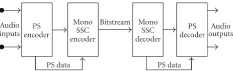
Figure20: Structure of the SSC encoder (left) and decoder (right) extended with PS. The PS encoder generates a down-mix and PS parameters. The resulting down-mix is subsequently encoded using a mono SSC encoder. The resulting mono bit stream and the PS parameters are combined into a single output bit stream. At the decoder side, the mono SSC decoder generates a time-domain down-mix signal, which is converted to stereo by a PS decoder based on the transmitted PS data.
3.2.1. Stereo Analysis
Overview. The PS encoder proceeds the SSC encoder (see
Figure 20). The PS encoder compares the two input signals
(left and right) for corresponding time/frequency tiles. The frequency bands are designed to approximate the psychoa-coustically motivated ERB scale, while the length of the segments is closely matched to known limitations of the binaural hearing system (see [53, 54]). Essentially, three parameters are extracted per time/frequency tile, represent-ing the perceptually most important spatial properties.
(i) Interchannel Level Difference (ILD), representing the level difference between the channels similarly to the “pan pot” on a mixing console.
(ii) Interchannel Phase Difference (IPD), representing the phase difference between the channels. In the frequency domain this feature is mostly interchange-able with an Interchannel Time Difference (ITD). The IPD is augmented by an additional Overall Phase Difference (OPD), describing the distribution of the left and right phase adjustment.
(iii) Interchannel Coherence (ICC), representing the coherence or cross-correlation between the channels.
While the first two parameters are coupled to the direction of sound sources, the third parameter is more associated with a spatial diffuseness (or width) of the source. Subsequent to parameter extraction, the input signals are down-mixed to form a mono signal. The down-mix can be made by trivial means of a summing process, but preferably more advanced methods incorporating time alignment and energy preservation techniques are incorporated to avoid potential phase cancellation (and hence resulting timbre changes) in the down-mix. The down-mix is subsequently encoded using a mono SSC encoder resulting in a mono bit stream. The PS data are properly quantized according to perceptual criteria [54], while redundancy is removed by means of Huffman coding. Finally, the mono SSC bit stream is combined with the PS data into a joint output bit stream.
3.2.2. Stereo Synthesis
Overview. The SSC decoder extended with a PS decoder is also outlined in Figure 20 and basically comprises the reverse process of the corresponding encoder. The SSC decoder generates a mono down-mix. Subsequently, the PS decoder reconstructs stereo output signals based on the PS parameters.
The PS decoder is outlined in more detail in Figure 21. The input signal (a mono decoded signal resulting from the SSC decoder) is processed by a hybrid analysis QMF bank. The hybrid QMF analysis bank is the same as used in HE-AAC (in SBR), extended with a second filter step to increase the spectral resolution for low frequencies according to psychoacoustical requirements (cf. [55]). The resulting subband signals are subsequently processed by a decorre-lation filter and a mixing stage. The decorredecorre-lation filter generates a artificial side signal based on the mono down-mix. The design of the decorrelation process is technically related to artificial reverberators but also includes many PS integration aspects due to, for example, the dynamics of the control parameters. This is thoroughly discussed in [56]. The hybrid QMF-domain output signals are obtained as a certain linear combination of the mono and side signal. This linear combination, referred to as mixing or rotation, is controlled by the PS parameters (ILDs, IPD/OPDs, ICCs). This process of up-mixing the mono signal, Mk,i with aid from the decorrelated mono signal,Dk,i, into the final estimate of left and right signal (Lk,i,Rk,i) is expressed by
⎡ ⎣Lk,i
Rk,i ⎤ ⎦=Hk,i
⎡ ⎣Mk,i
Dk,i ⎤
⎦ (7)
using the up-mix matrixHaccording to
Hk,i= ⎡ ⎣h11 h12
h21 h22
⎤
⎦, (8)
wherekandidenote the frequency subband and the QMF time slot, respectively. The elements in the up-mix matrix,
Hk,i are the only up-mix variables actually derived from the stereo parameters. Details about the calculation of these matrix elements can be found in [36,54,57]. Finally, two hybrid QMF banks are used to generate the two output signals.
3.3. SSC Performance. In order to be included in the MPEG-4 standard, the developed high-quality parametric coder needed to pass the requirements that were set out at the start of the standardization process. These requirements were twofold.
(i) The coder should provide the same quality in the mean at a 25% less bit rate compared to the existing MPEG-4 state-of-the-art technology.
Bitstream SSC decoder
Hybrid QMF analysis
PS data
Decorr. filter
PS decoder
Mixing
Hybrid QMF synthesis
Hybrid QMF synthesis
Audio outputs
Figure21: Structure of the QMF-based PS decoder. The signal is first fed through a hybrid QMF analysis filter bank. The filter-bank output and a decorrelated version of each filter-bank signal is subsequently fed into the mixing and phase-adjustment stage. Finally, two hybrid QMF banks generate the two output signals.
50 40 30 20 10
Bit rate (kbps) 1
2 3 4 5
MOS
Anchors
Figure22: Average scores (MOS) versus bit rate for coded stereo signals. The filled circles indicate the SSC coder (at 16, 20, and 24 kbps), the stars the AAC coder (at 24, 32, and 48 kbps). The open circles on the right-hand side are the anchors (hidden reference, 7 kHz and 3.5 kHz low-pass filtered versions from top to bottom, resp.). The 95% confidence intervals have as typical range 0.3 MOS units. Adapted from [58].
The existing MPEG-4 state-of-the-art technology at that moment in time was AAC.
These requirements have been assessed in a subjective verification test conducted by the Instit¨ut f¨ur Rundfunktech-nik (IRT). In this section we present some of the results that were reported at that point in time. The data that are discussed are taken from [58].
The listening tests performed for the MPEG-4 standard-ization were done in two stages. A set of 53 critical items were encoded using the SSC (from Philips) and the AAC encoder (Fraunhofer Gesellschaft, FhG), respectively. The encoding was done at different bit rates and for mono as well as stereo material. The Instit¨ut f¨ur Rundfunktechnik (IRT) did a prescreening test to generate a set of 9 critical items to be included in the final listening test which was also executed at IRT. Here, we discuss only the results of this final listening test obtained with the stereo input material, since this is the more relevant data from an application point-of-view. Furthermore, the results from an additional listening test performed at Philips concerning all 53 tests items are presented.
Next to the 9 encoded items, the IRT test included the hidden reference and two anchors, being the original mate-rial band-limited at 3.5 and 7 kHz. The test was performed with headphones using 26 listeners. The MUSHRA tool was used and the listeners were instructed to give a Mean Opinion Score (MOS).
The test was supposed to be a blind test. However, since two completely different coding strategies were used, the test was effectively far from blind. The AAC coder reduces its bandwidth when operating at low bit rates and this is always immediately recognized unless there is band-limited material. The SSC encoder never uses a band limitation, this being an ingredient for reaching a high quality encoding. The completely different artifacts introduced by both coding schemes effectively not only prohibit a blind comparison, but also made the ranking of the different coders a complicated task. Also, the results tend to be subject-dependent. For example, in older experiments involving SSC and AAC performed at Philips we found that listeners that are well-acquainted with band-limitations (speech-coding experts) tended to perceive the AAC band limitation as less annoying than most other listeners.
The SSC coder was operated at 16, 20, and 24 kbps, the AAC coder at 24, 32, and 48 kbps. InFigure 22the results can be found. The crosses indicate the mean score of the AAC coder, the filled circles those of the SSC coder and the open circles on the right reflect the mean of the anchors. The 95% confidence intervals are indicated as well for the AAC and SSC means. Interestingly, the AAC score is dropping rapidly as a function of bit rate, whereas the quality of the SSC coder is not. Comparing AAC at 24 kbps with SSC at the same bit rate, it is clear that the first is statistically significant better. The MOS score for SSC is on the border of a fair and good qualification. According to this test, the score of SSC at 24 kbps is roughly equivalent to that of AAC at 32 kbps. However, in view of the fact that some of the 9 excerpts were rather band-limited [58], we decided to look in somewhat more detail to this comparison.