The Thirty-Third AAAI Conference on Artificial Intelligence (AAAI-19)
One-Network Adversarial Fairness
Tameem Adel
University of Cambridge, UK [email protected]
Isabel Valera
MPI-IS, Germany [email protected]
Zoubin Ghahramani
University of Cambridge, UK Uber AI Labs, USA [email protected]
Adrian Weller
University of Cambridge, UK The Alan Turing Institute, UK
Abstract
There is currently a great expansion of the impact of machine learning algorithms on our lives, prompting the need for ob-jectives other than pure performance, including fairness. Fair-ness here means that the outcome of an automated decision-making system should not discriminate between subgroups characterized by sensitive attributes such as gender or race. Given any existing differentiable classifier, we make only slight adjustments to the architecture including adding a new hidden layer, in order to enable the concurrent adversarial op-timization for fairness and accuracy. Our framework provides one way to quantify the tradeoff between fairness and accu-racy, while also leading to strong empirical performance.
1
Introduction
Automated decision support has become widespread, raising concerns about potential unfairness. Here, following earlier work, unfairness means discriminating against a particular group of people due to sensitive group characteristics such as gender or race (Grgic-Hlaca et al. 2018b; Hardt, Price, and Srebro 2016; Kusner et al. 2017; Louizos et al. 2016; Zafar et al. 2017c; 2017a; Zemel et al. 2013). Fairness con-cerns have been considered in applications including pdictive policing (Brennan, Dieterich, and Ehret 2009), re-cidivism prediction (Chouldechova 2017) and credit scor-ing (Khandani, Kim, and Lo 2010). The current trend in the literature on fairness is to begin with a notion (definition) of fairness, and then to construct a model which automates the detection and/or eradication of unfairness accordingly. Common definitions of fairness consider whether or not a decision is related to sensitive attributes, such as gender.
Most state-of-the-art machine learning algorithms for fair-ness build from scratch a model’s architecture tailored for a specific fairness notion. In contrast, we propose a method that slightly modifies the architecture of the model which was to be optimized solely for accuracy. We learn a fair rep-resentation together with a new performance function acting on it, with the goal of concurrently optimizing for both fair-ness and performance (accuracy). Our method is based on an adversarial framework, which allows explicitly measuring the tradeoff between fairness and accuracy. Our approach
Copyright c2019, Association for the Advancement of Artificial
Intelligence (www.aaai.org). All rights reserved.
is general, in that it may be applied to any differentiable dis-criminative model. We establish a fairness paradigm where the architecture of a deep discriminative model, optimized for accuracy, is modified such that fairness is imposed (the same paradigm could be applied to a deep generative model in future work). Beginning with an ordinary neural network optimized for prediction accuracy of the class labels in a classification task, we propose an adversarial fairness frame-work performing a change to the netframe-work architecture, lead-ing to a neural network that is maximally uninformative about the sensitive attributes of the data as well as predic-tive of the class labels. In this adversarial learning frame-work, there is no need for a separate network architecture representing the adversary, thus we avoid the well-known difficulties which may arise from double-network adversar-ial learning (Goodfellow 2016; Goodfellow et al. 2014).
We make the following contributions: 1) We propose a fairness algorithm by modifying the architecture of a poten-tially unfair model to simultaneously optimize for both ac-curacy and fairness with respect to sensitive attributes (Sec-tion 2); 2) We quantify the tradeoff between the accuracy and fairness objectives (Section 2); 3) We propose a vari-ation of the adversarial learning procedure to increase di-versity among elements of each minibatch of the gradient descent training, in order to achieve a representation with higher fidelity. This variation may be of independent inter-est since it is applicable generally to adversarial frameworks (Section 2.2); 4) We develop a novel generalization bound for our framework illustrating the theoretical grounding be-hind the relationship between the label classifier and the ad-versary’s ability to predict the sensitive attribute value (Sec-tion 3); and 5) We experiment on two fairness datasets com-paring against many earlier approaches to demonstrate state-of-the-art effectiveness of our methods (Section 4).
2
Fair Learning by Modifying
an Unfair Model
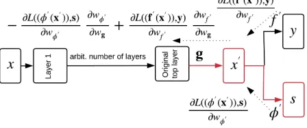
is invariant to changes in the sensitive attribute values. To optimize this invariance, an adversary is included at the top of the model in the form of a classifier which tries to predict the sensitive attribute value. For a deep model, this can be implemented via: (i) adding another classifier at the top of the network such that we have two classifiers: the original label predictor and the new predictor of sensitive attribute value(s); and (ii) adding a network layer just under the clas-sifiers (now the top hidden layer) that aims at maximizing the performance of the label predictor, while minimizing the performance of the sensitive attribute predictor by reversing the gradients of the latter in the backward phase of the gra-dient descent training. See Figure 1 for an illustration.
2.1
Fair adversarial discriminative (
FAD
) model
We consider dataD = {(xi,yi,si)}ni=1, wherexi,yiand
sirefer to the input features, the ground truth label and the
sensitive attribute(s), respectively. Denote by yˆi the
corre-sponding label estimate. Typically speaking,yˆiis predicted
by a potentially unfair discriminative classifier possibly rep-resented by a neural network whose input is featuresxand sensitive attributess. The goal of fairness is to ensure that the prediction of y is not dependent on these attributes s
(Zafar et al. 2017c). A naive approach is to simply dis-card s and let classifier f have input x - this has some proponents in terms of process (Grgic-Hlaca et al. 2018a; 2018b) but suffers sincexmight include significant infor-mation abouts. For example, an address attribute inxmight give a strong indication about races.
We achieve fairness through the adversarial construction illustrated in Figures 1 and 2, as follows. Define the em-pirical classification loss of the label classifier f0(x0) as
L(ˆy,y) = L(f0(x0),y) = |D1|P|D|
i=1Err(f 0(x0
i),yi), and
similarly the classification loss of the classifierφ0,
predict-ing the value of the sensitive attributes, asL(φ0(x0),s) =
1 |D|
P|D|
i=1Err(φ0(x0i),si). A simplified view of the
ar-chitecture of our fairness adversarial discriminative (FAD) framework is displayed in Figure 1. We extend the original architecture of the potentially unfair predictor, by adding a new layergthat produces a fair data representationx0, and adding a new predictor φ0 aiming to predict the sensitive attributes. Denoting by w the weight vector of a network layer, the backpropagation forward pass proceeds normally inFAD. During the backward pass (dotted lines), however, the gradient from the loss of thesclassifier ∂L(∂wφ0(x0),s)
φ0 is
multiplied with a negative sign so thatgadversarially aims at increasing the loss ofφ0, resulting in a representationx0
maximally invariant to the change in values ofs. Since the rest of theFADtraining proceeds normally, the classifierf0
should also makex0 maximally informative about the
orig-inal prediction task, depicted byy. The idea of reversing a layer’s gradient with respect to the layer below in the back-ward pass was used in domain adaptation to develop invari-ant representations to changes between the source and target domains (Ajakan et al. 2014; Ganin and Lempitsky 2015; Ganin et al. 2016).
In our fairness paradigm, we aim at the following: i)
achieving fairness; ii) quantitatively evaluating how much fairness we achieve, and; iii) quantifying the impact of such fairness on accuracy, i.e. computing the difference in accu-racy between the proposed fair model and a corresponding (potentially unfair) model. In Figure 2, another schematic di-agram of the proposed modifications is displayed. The pre-dictorφ0(x0)depicts a classifier predicting thesvalue from
x0. The ability to accurately predictsgivenx0 signifies a high risk of unfairness since this means that the sensitive at-tributes may be influential in any decision making process based onx0. Adversarially throughg, the non-sensitive fea-tures xare transformed into a representation x0 which at-tempts to break any dependence on the sensitive attributes
s. As such, the optimization objective can have many triv-ial solutions, e.g.gthat maps everyxinto0which provides no information to predicts. In order to prevent that, and to ensure that fairness is rather aligned with the accuracy ob-jective, a classifierf0predicts the labelsyfromx0. Here we consider classification accuracy to be the metric of the ini-tial model. However, our adversarial paradigm can also be adopted in models with other metrics to achieve fairness.
Figure 1: Architecture of the proposed fair adversarial dis-criminative model. The parts added, due to FAD, to a po-tentially unfair deep architecture with inputxare (shown in red): i) the layergwherex0is learned and; 2) the sensitive attribute spredictor φ0 at the top of the network. Denote
bywthe weight vector of the respective layer. The forward pass of backpropagation proceeds normally inFAD. During the backward pass (dotted lines), the gradient from the loss of thesclassifier ∂L((φ
0(x0)),s)
∂wφ0 is multiplied with a negative sign so that gadversarially aims at increasing the loss of
φ0, resulting in a representation x0 maximally invariant to the change in values ofs. The rest of theFADtraining pro-ceeds normally, i.e. gradient from the labeling classifierf0,
∂L((f0(x0)),y)
∂wf0 , is normally (with a positive sign) imported to
g, ultimately makingx0maximally informative abouty.
To summarize: g,φ0 andf0 are all involved in the con-current optimization for fairness and accuracy. The param-eters ofgandφ0 adversarially optimize for fairness while
Figure 2: The proposed FAD
paradigm. We establish an ad-versarial objective whereg mini-mizes the ability of the predictor
φ0 to correctly predict values of the sensitive attributess, whereas
φ0 on the other hand maximizes its own accuracy in predictings. Another predictorf0 predicts the labelsyfromx0.
f0(x0)obtained after learningg, andf(x), respectively.
Fairness notions We focus on two common notions (def-initions) of fairness, disparate impact (Barocas and Selbst 2016; Feldman et al. 2015; Primus 2010) and
disparate mistreatment (Zafar et al. 2017b). We
first address the former. Disparate impact refers to a deci-sion making process that, in aggregate, leads to different out-comes for subpopulations with different sensitive attribute values. According to this notion, and assuming WLOG a binary label and sensitive attribute, fairness is achieved (in other words, there is no disparate impact) when:
p(ˆy= 1|s= 0) =p(ˆy= 1|s= 1). (1)
For our proposed model, define the part of the data D
where s = 0 as Ds=0, then p(ˆy = 1|s = 0) = 1
|Ds=0|
P|Ds=0|
i=1 p(f0(x0) = 1). Accordingly, disparate
im-pact is avoided when:
1 |Ds=0|
P|Ds=0| i=1 p(f
0(x0) = 1) = 1 |Ds=1|
P|Ds=1| i=1 p(f
0(x0) = 1) (2)
The disparity (Disp) between both sides of (2) quantifies unfairness in terms of disparate impact. Larger disparity val-ues signify more unfairness:
DispDI= (3)
1 |Ds=0|
P|Ds=0|
i=1 p(f0(x0) = 1)− 1 |Ds=1|
P|Ds=1|
i=1 p(f0(x0) = 1)
The other notion of fairness we inspect is referred to as
disparate mistreatment (Zafar et al. 2017b). One
major difference between the two notions is that disparate mistreatment depends on the ground truth labels y, and therefore it can be considered only when such information is available. Assuming a binary labelywith ground truth val-ues1and−1, disparate mistreatment arises when the rate of erroneous decisions (false positives, false negatives or both) is different for subpopulations with different values of sensi-tive attributes. Unfairness in terms of disparate mistreatment is thus avoided when the false positive rate (FPR) and false negative rate (FNR) are as in (4) and (5), respectively.
p(ˆy6=y|y=−1,s= 0) =p(ˆy6=y|y=−1,s= 1) (4)
p(ˆy6=y|y= 1,s= 0) =p(ˆy6=y|y= 1,s= 1) (5)
A larger disparity between both sides in either of these two equations signifies more disparate mistreatment. For our model, disparate mistreatment, as a whole, is defined in (6).
1 |Ds=0|
P|Ds=0|
i=1 Err(f0(x0i),yi) =|D1s=1|
P|Ds=1|
i=1 Err(f0(x0i),yi)
(6)
Decomposing (6) into FPR and FNR is straightforward. The higher the following disparity values the more unfair the model is, in terms of disparate mistreatment:
DispFPR= (7)
1 |Ds=0|
P|Ds=0| i=1 Err(f
0(x0
i),yi|yi=−1)−|D1
s=1|
P|Ds=1| i=1 Err(f
0(x0
i),yi|yi=−1)
DispFNR= (8)
1 |Ds=0|
P|Ds=0|
i=1 Err(f0(x0i),yi|yi=1)−|D1
s=1|
P|Ds=1|
i=1 Err(f0(xi0),yi|yi= 1)
Modeling objective The overall training objective of the proposed model, for a dataset of sizen, is stated as follows:
ming,f0[L(f0(g(x)),y)−βmaxφ0(L(φ0(g(x)),s))] ≡ (9)
ming,f01
n
Pn
i=1Err(f0(g(xi)),yi)−βmaxφ0 1
n
Pn
i=1Err(φ0(g(xi)),si)
,
where the fairness hyperparameterβ >0controls the degree of fairness induced in the model.
The model, as such, is based on optimizing for disparate impact. Recall that the whole proposed model is ultimately implemented as one neural network in which the adversarial layer gis injected as a hidden layer right beneath the top layer consisting of the classifiersφ0andf0.
In order to optimize for disparate mistreatment, a modi-fication to (9) is needed. The functionφ0(x0) = φ0(g(x)) should be multiplied by a term reflecting what is needed to be equal for subpopulations with different sensitive attribute values such that disparate mistreatment is achieved. Multi-plying φ0(g(x))with the ratio of Err(f0(x0i),yi) over n,
which signifies the misclassification rate, leads to the objec-tive becoming an interpretation of disparate mistreatment. The overall training objective when optimizing for disparate mistreatment therefore becomes:
ming,f01
n
Pn
i=1Err(f0(g(xi)),yi)−βmaxφ0 1
n
Pn
i=1Err(φ0(g(xi)),si)I(ˆyi6=yi)
, (10)
whereI(z)is the indicator function:I(z) = 1, whenzis true and0otherwise. However, sinceyˆis the classification output, which depends on bothgandf0, the indicator func-tion might be problematic to optimize by gradient descent. Hence, we can relax this optimization problem and rewrite it as follows to express the labeling misclassification proba-bility:
ming,f01
n
Pn i=1Err(f
0(g(x
i)),yi)−βmaxφ0 1
n
Pn i=1Err(φ
0(g(x
i)),si)p(ˆyi6=yi)
≡
ming,f0 h
1
n
Pn
i=1Err(f0(g(xi)),yi)−βmaxφ0
Pn
i=1
Err(f0(x0 i),yi)
n Err(φ
0(g(x i)),si)
i
(11)
For the decomposition of disparate mistreatment into FPR and FNR, the term Err(f0(x0i),yi) = Err(f0(g(xi)),yi)
in (11) shall be divided into Err(f0(x0i),yi)yi=0 and Err(f0(x0i),yi)yi=1, respectively.
Goodfellow et al. 2014). Imagine if the input to the discrim-inator is MNIST images, and, instead of covering the whole space of the ten digits, the comparisons are restricted to two or three digits that are ultimately being represented quite similarly by data of both classes introduced as input to the discriminator. The latter therefore becomes maximally con-fused and a convergence of the whole adversarial learning framework is reached although in reality only a small subset of the data is well represented by the inferred representa-tion. Since we want to avoid imposing too many variations on the original settings of the system, we need to develop a computationally efficient solution to mode collapse. Most of the previously proposed solutions are either tailored to the generative versions of adversarial learning (Arjovsky, Chin-tala, and Bottou 2017; Kim et al. 2017; Metz et al. 2017; Rosca et al. 2017) or computationally inefficient for our purpose (Srivastava et al. 2017). We experimented with the heuristics proposed in (Salimans et al. 2016) but they did not improve results in our one-network adversarial framework.
Therefore we propose a method based on making ele-ments of a minibatch as diverse as possible from one an-other. Each minibatch is formed as follows: i) Beginning with very few data points randomly chosen to belong to the minibatch, there is a pool of points from which some are to be selected for the addition to the minibatch based on the criterion of ending up with minibatch elements as diverse as possible without losing too much in terms of computational runtime; ii) A point is selected from the pool via the score resulting from a one-class support vector machine (SVM) classifier where the class consists of the current elements of the minibatch. The next added data point from the pool to the minibatch is the point with the lowest score, i.e. the point be-lieved to be the least likely to belong to the class formed by the current minibatch elements, or the most dissimilar point to the minibatch elements; iii) This process continues until greedily reaching the prespecified size of the minibatch. The size of each pool of points to begin with is a hyperparameter to be specified by e.g. cross-validation. We claim that using the efficient one-class SVM to form minibatches is a step in the direction of establishing adversarial learners with a bet-ter coverage of all the regions of the data space.
3
Generalization Bound
We illustrate the theoretical foundation of the relationship between the label classifier and the adversary’s ability to predict the sensitive attribute value. We begin by deriving a generalization upper bound for the framework (Theorem 1). We shed light on the interpretation of the sensitive attribute classifier as an adversary in the concurrent adversarial opti-mization for fairness and accuracy, in terms of the distance between data distributions given different sensitive attribute values.
Assume the label y (as well as its estimate yˆ) and the sensitive attribute s values are binary. Recall that a data sample D = {(xi,yi,si)}ni=1 is given. Also, recall that,
for the ith instance, the classification loss between yˆ and
y (equivalently defined between any two labelings) is de-noted by Err(ˆyi,yi). Denote the expected loss between
two labelingsyˆ andywith respect to a distribution Pby
LP(ˆy,y) =EP[Err(ˆy,y)]. When abbreviated asErr(ˆy),
this means that the other side is the ground truth labely. Next we describe the Rademacher complexity, which measures the richness of a class of real-valued functions with respect to a probability distribution (Shalev-Shwartz and Ben-David 2014).
Rademacher complexity facilitates the derivation of gen-eral learning guarantees for problems with infinite hy-pothesis sets, like ours. Thanks to the introduction of a Rademacher random variable σ, Rademacher complexity directly maps the measurement of accuracy (or inversely error rate) of the hypothesis into the richness or expres-siveness of the hypothesis w.r.t. the probability distribu-tion resulting from the introducdistribu-tion of σ. More formally, let H be a hypothesis set, where h ∈ H is an arbitrary hypothesis of the set. Define the expected loss of a hy-pothesis class as Err(H)1. When each his a real-valued function, the empirical Rademacher complexity (Mansour, Mohri, and Rostamizadeh 2009; Mohri and Afshin 2008a; Shalev-Shwartz and Ben-David 2014) ofHgivenDcan be defined as:
RadD(H) =
1
nEσ[ suph∈H n
X
i=1
σih(xi)], (12)
where σ1, σ2, · · ·, σn are independent random variables drawn from the Rademacher distribution, which notes that
P r(σ= 1) =P r(σ=−1) = 0.5. TheRademacher com-plexityof a hypothesis setHis thence denoted by the expec-tation ofRadD(H)over all samples of sizen:
Radn(H) =ED[RadD(H)] (13)
For deriving our bound, we use a notion of distance be-tween distributions, proposed by Mansour, Mohri, and Ros-tamizadeh (2009), and referred to as the discrepancy dis-tance. It is symmetric and it satisfies the triangle inequal-ity. Denote byHa hypothesis set, where eachh ∈ His a classifierX → Y. The discrepancy distance between two arbitrary distributionsPandQis defined as:
disc(P,Q) = max
h,h0∈H|LP(h,h
0)−L
Q(h,h0)| (14)
We also state the following bound (Bartlett and Mendelson 2002; Koltchinskii and Panchenko 2000), whose proof is in (Bartlett and Mendelson 2002). For a probability distribu-tionP(estimated byPˆ) defined onX× {±1}, letHbe a hypothesis set where eachh ∈ His a{±1}-valued func-tion mappingXto a binaryY. Then for a data sampleD
with sizen, With probability at least1−δ, and for a 0-1 classification loss, every hypothesish∈Hsatisfies:
EP(Err(Y,h(X)))≤EPˆ(Err(Y,h(X))) +
RadD(H)
2
+
r
log(1/δ)
2n (15)
1
Note that this is the expectation of a class of functions with
respect to a specific data sampleD. This differs fromLP(h(x),y)
since the latter is the expectation of a specific functionhwith
Theorem 1. Denote by P0 and P1 the distributions
P(x|s= 0)andP(x|s= 1), respectively. Assuming train-ing dataD with size n, which, without loss of generality (WLOG), is equally divided into data points withs= 0,D0,
and those withs= 1,D1. For a classHof binary
classi-fiers, and forδ >0with probability greater than or equal to 1−δ, the following holds:
disc(P0,P1)≤disc( ˆP0,Pˆ1) + 2
r
log(1/δ)
n
+1
2(RadD0(Err(H))+RadD1(Err(H))) (16)
Proof. Using the triangle inequality, the L.H.S. of (16) can turn into:
disc(P0,P1)≤disc(P0,Pˆ0) +disc(P1,Pˆ1) +disc( ˆP0,Pˆ1)
(17)
For a 0-1 classification error, we can use (15) with the class of real-valued functions being a class where each ele-ment is the loss ofh,Err(h), on a specific training sample
D, instead ofhitself. We can as well replaceyin (15) with an arbitraryh, and since we are upper bounding we can as-sume we replace it with the worst caseh, i.e.hresulting in the highest upper bound. This leads to:
EP(Err(h(x),h0(x)))≤EPˆ(Err(h(x),h0(x)))
+RadD(Err(H))
2 +
r
log(1/δ) 2n
(18)
Since EP(Err(h(x),h0(x))) = LP(h(x),h0(x)), and
from (14), then (18) turns into:
disc(P,Pˆ)≤ RadD(Err(H))
2 +
r
log(1/δ)
2n (19)
Using (19) to describe the terms disc(P0,Pˆ0) and
disc(P1,Pˆ1)in (17), we get:
disc(P0,P1)≤disc( ˆP0,Pˆ1)
+RadD0(Err(H))
2 +
r
log(1/δ)
n
+RadD1(Err(H))
2 +
r
log(1/δ)
n
(20)
disc(P0,P1)≤disc( ˆP0,Pˆ1) + 2
r
log(1/δ)
n
+1
2(RadD0(Err(H)) +RadD1(Err(H))) (21)
which concludes the proof.
This provides an interpretation of our modeling objective in (9) in the main document, since: The sensitive attribute classifierφ0(g(x))aims at minimizing the first term in the
bound on the right of (21),disc( ˆP0,Pˆ1). The label
classi-fierf0(g(x))aims at minimizing the second term on the right of (21). The third term on the right of (21) tends to zero as the sample sizengoes to infinity.
To further clarify that: As noted in (Mansour, Mohri, and Rostamizadeh 2009), for a 0-1 classification error and for our hypothesis class consisting of the loss on each hy-pothesis,Err(h), the discrepancy distancedisc( ˆP0,Pˆ1)is
equivalent to the following notion of distance, referred to as H-divergence (Ben-David et al. 2007; 2010; Devroye, Gy-orfi, and Lugosi 1996; Kifer, Ben-David, and Gehrke 2004):
dH( ˆP0,Pˆ1) = sup
a∈|h−h0|
|Pˆ0(a)−Pˆ1(a)| (22)
As proved in (Ben-David et al. 2007; 2010) (Lemma 2 in (Ben-David et al. 2010)), theH-divergence in such case can be approximated by performing a classification task of the dataDinto points belonging toD0or toD1:
dH( ˆP0,Pˆ1) = 2(1−min h
h2
nI(x∈D0) +
2
nI(x∈D1)
i
)
(23)
where the distance (H-divergence, which is equivalent in this case to the discrepancy distance) between Pˆ0andPˆ1
is inversely proportional to the performance of the classifier. From (21) and (23), for an arbitraryh:
disc(P0,P1) ≤2−
h4
nI(x∈D0) +
4
nI(x∈D1)
i
+1
2(RadD0(Err(H)) +RadD1(Err(H)))
+ 2
r
log(1/δ)
n (24)
The termhn4I(x∈D0) +n4I(x∈D1)
i
is what is estimated in our proposed formulation in (9) in the main document by −β maxφ0(L(φ0(g(xi)),si)). Due to the negative sign pre-ceding the latter term in (9) and the equivalent former term in (24), it is inversely proportional to the maximization of our objective, and to the overall distance between estimated dis-tributions of data with differentsvalues, respectively. Also, the larger the value of the fairness hyperparameter β, the higher the impact of this term on the optimization of our ob-jective.
The label classifierf0(g(xi))aims at minimizing the er-ror of the classifier, i.e. minimizing the erer-ror in predict-ing the labelyˆ of the data points D (bothD0andD1). It
is therefore straightforward to see that f0(g(xi))naturally aims at minimizing the second term in the bound in (21), (RadD0(Err(H)) +RadD1(Err(H))).
4
Experiments
On two datasets, we perform experiments to evaluate the following: (i) the difference in classification accuracy due to optimizing for fairness–Table 1 and Figure 3. Compar-isons among the unfair and fair versions of the proposed frameworks,FADandFAD-MD, as well as previous state-of-the-art algorithms, show that the quest for fairness with
FAD andFAD-MD leads to minimal loss in accuracy; (ii)
(un)fairness, in terms of both disparate impact and disparate mistreatment–Table 2. Results demonstrate state-of-the-art effectiveness of FAD and FAD-MD; and (iii) an MMD 2-sample test to assess the fidelity of the learned fair repre-sentationx0–Figure 4. This also shows the effectiveness of
increasing the minibatch diversity in FAD-MD. Moreover, the increase in training time due to optimizing for fairness is not considerable forDAFcompared to its unfair version.
We test our framework on two popular real-world datasets in the fairness literature, the Propublica COMPAS dataset (Larson et al. 2016) and the Adult dataset (Dheeru and Taniskidou 2017). The task in the COMPAS dataset is a bi-nary classification task with two classes depicting whether or not a criminal defendant is to recidivate within two years. We use the black vs. white values of the race feature as our sensitive attribute. The total number of the COMPAS data instances we work on is 5,278 instances and 12 features. On the other hand, the Adult dataset consists of 32,561 com-plete instances denoting adults from the US Census in 1994. The task is to predict, from 14 features, whether an adult’s income is higher or lower than 50K USD. Gender is the sen-sitive attribute in the Adult data (male or female). Each ex-periment is repeated ten times where, in each run, data is randomly split into three partitions, training, validation (to identify the value of the fairness hyperparameterβ) and test. A portion of 60%of the data is reserved for training, 20% for validation and 20%for testing. Statistics reported are the averages of the ten repetitions. For FAD-MD, we use the one-class SVM introduced in (Scholkopf et al. 2000) with
ν= 0.5(fractions of support vectors and outliers).
On both datasets, and in addition to the unfair versions of the proposed algorithms, of (Zafar et al. 2017b) and of (Zafar et al. 2017a), we compare (where applicable) FAD
and FAD-MD to the following state-of-the-art fairness
al-gorithms: Zafar et al. (2017b), Zafar et al. (2017a), Za-far et al. (2017c), Hardt, Price, and Srebro (2016), Feld-man et al. (2015), Kamishima et al. (2012), Fish, Kun, and Lelkes (2016), Bechavod and Ligett (2017), Komiyama et al. (2018), Agarwal et al. (2018), Narasimhan (2018). Clas-sification results are displayed in Table 1. A 2-layer neural network is utilized to obtain the results of the unfair clas-sification, whereas the adversarial layer is added under the top layer to accomplish fairness viaFADand its variation
FAD-MD. Values of the fairness hyperparameterβ selected
by cross-validation are 0.3 and0.8 for the COMPAS and Adult datasets, respectively. Classification results on both datasets demonstrate that, among fairness algorithms,FAD
andFAD-MDachieve state-of-the-art classification accuracy.
In addition, the impact on classification accuracy due to the optimization for fairness by the proposed algorithms,FAD
andFAD-MD, is rather minimal. This is quantified via the
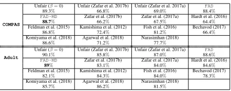
Table 1: Results of the classification accuracy on the COM-PAS and Adult datasets. In addition to its impact on fairness, increasing the minibatch diversity with FAD-MDimproves the classification accuracy. Classification accuracy values achieved byFADandFAD-MDon both datasets are higher than previous state-of-the-art results. Loss in accuracy due to fairness (difference in classification accuracy between the unfair and fair versions) is not big; with FAD-MD, it is as minimal as state-of-the-art by Zafar et al. (2017b) for the COMPAS data, and uniquely minimal for the Adult data. Bold refers to an accuracy value that is significantly better than the other fair (all apart from the first three entries) com-petitors. To test significance, we perform a paired t-test with significance level at5%.
COMPAS
Unfair (β= 0) Unfair (Zafar et al. 2017b) Unfair (Zafar et al. 2017a) FAD
89.3% 66.8% 69.0% 88.4%
FAD-MD Zafar et al. (2017b) Zafar et al. (2017a) Hardt et al. (2016)
88.7% 66.2% 67.5% 64.4%
Feldman et al. (2015) Kamishima et al. (2012) Fish et al. (2016) Bechavod (2017)
86.8% 72.4% 81.2% 66.4%
Komiyama et al. (2018) Agarwal et al. (2018) Narasimhan (2018)
86.6% 71.2% 77.7%
Adult
Unfair (β= 0) Unfair (Zafar et al. 2017b) Unfair (Zafar et al. 2017a) FAD
90.1% 85.8% 87.0% 88.6%
FAD-MD Zafar et al. (2017b) Zafar et al. (2017a) Hardt et al. (2016)
89% 83.1% 84.0% 84.6%
Feldman et al. (2015) Kamishima et al. (2012) Fish et al. (2016) Bechavod (2017)
82.1% 84.3% 84.0% 78.3%
Komiyama et al. (2018) Agarwal et al. (2018) Narasimhan (2018)
85.7% 86.2% 81.5%
difference in accuracy between the unfair and fair versions of the proposed framework compared to such difference in the cases of (Zafar et al. 2017b) and (Zafar et al. 2017a).
In Figure 3, we vary the classification accuracy as a func-tion of the fairness hyperparameter β.FAD-MDleads to a slightly higher classification accuracy thanFAD. Classifica-tion accuracy initially decreases when optimizing for fair-ness until it rather saturates with larger values ofβ.
Fairness results, in the form of empirical values of the dis-parity notions described in (3), (7) and (8), are displayed in Table 2. Such values are shown forFAD,FAD-MDand the same competitors as in Table 1, where applicable. The proposed algorithms,FADandFAD-MD, minimize the dis-parity values (unfairness) when optimizing for fairness, and achieve the (at times joint) best results, in terms of the fair-ness metrics, in five out of six cases (three disparity values -DispDI,DispFPRand DispFNR- for each dataset).
We move on now to a more rigorous evaluation of the minibatch diversity augmentation byFAD-MD. One of the problems of most current frameworks of adversarial learn-ing is the fact that the adversary bases its optimization on comparing data points instead of distributions or, at least, of sets of points. We aim at evaluating this here by per-forming a nonparametric two-sample test between represen-tations of data points belonging to different values of the sensitive attribute s. The null hypothesis denotes that the distributions of the learned representation x0 given differ-entsvalues are equal,H0 : p(x0|s = 0) = p(x0|s = 1),
and its alternative is H1 : p(x0|s = 0) 6= p(x0|s = 1).
Failing to reject (i.e. accepting) the null hypothesis H0 is
maxi-Table 2: Unfairness of different algorithms measured by disparate impact -DispDI in Eq. (3) and disparate mistreatment -DispFPR, DispFNRin Eqs. (7,8)- on the COMPAS and the Adult datasets. Smaller values are more favorable since they denote less unfairness. For each competitor, we report their best value achieved throughout their different settings. In five out of six cases (three disparity values for each dataset), the proposed algorithms,FADandFAD-MD, (at times jointly) achieve the best results in terms of the fairness metrics. Bold refers to a value that is significantly less (better) than its non-bold competitors. To test significance, we perform a paired t-test with significance level at5%. Empty cells indicate non-applicable experiments.
COMPAS
Unfair (β= 0) Unfair (Zafar et al. 2017b) Unfair (Zafar et al. 2017a) FAD FAD-MD Zafar et al. (2017b) Zafar et al. (2017a) Hardt et al. (2016) DispDI: 0.6 — 0.62 0.08 0.11 — 0.38 —
DispFPR: 0.21 0.18 — 0.01 0.01 0.03 — 0.01 DispFNR: 0.29 0.3 — 0.01 0.02 0.1 — 0.01 Feldman et al. (2015) Kamishima et al. (2012) Fish et al. (2016) Bechavod (2017) Komiyama et al. (2018) Agarwal et al. (2018) Narasimhan (2018)
0.95 0.9 0.15 — 0.2 0.09 0.1
0.4 0.2 0.03 0.01 — 0.05 0.09
0.45 0.15 0.03 0.03 — 0.05 0.11
Adult
Unfair (β= 0) Unfair (Zafar et al. 2017b) Unfair (Zafar et al. 2017a) FAD FAD-MD Zafar et al. (2017b) Zafar et al. (2017a) Hardt et al. (2016) DispDI: 0.71 — 0.68 0.14 0.13 — 0.29 —
DispFPR: 0.36 0.35 — 0.02 0.01 0.12 — 0.04
DispFNR: 0.32 0.4 — 0.01 0.02 0.09 — 0.03
Feldman et al. (2015) Kamishima et al. (2012) Fish et al. (2016) Bechavod (2017) Komiyama et al. (2018) Agarwal et al. (2018) Narasimhan (2018)
0.25 0.3 0.16 — 0.28 0.13 0.19
0.3 0.07 0.02 0.0 — 0.04 0.14
0.4 0.08 0.03 0.04 — 0.05 0.08
0.0 0.5 1.0 1.5 2.0 2.5 3.0 Value of the parameter 82
83 84 85 86 87 88 89 90
Cl
as
sif
ica
tio
n
ac
cu
ra
cy
(%
) COMPAS dataset
FAD FAD-MD
(a) COMPAS dataset
0.0 0.5 1.0 1.5 2.0 2.5 3.0 Value of the parameter 87.5
88.0 88.5 89.0 89.5 90.0 90.5
Cl
as
sif
ica
tio
n
ac
cu
ra
cy
(%
) Adult dataset
FAD FAD-MD
(b) Adult dataset
Figure 3: Classification accuracy as a function of the fair-ness hyperparameterβ, whereβ = 0indicates no adjust-ment for fairness. The COMPAS data is balanced; 47%of the instances have recidivated and 53%have not. Hence, a random guessing classifier’s accuracy would be as low as around 53%. For the Adult data, a random guessing classi-fier would result in 75.9% accuracy, since there are many more records for people whose income is less than or equal to 50K. Classification accuracy initially decreases with in-creasingβ until it saturates. With both datasets, classifica-tion accuracy has not considerably changed forβ >1. Ac-curacy achieved byFAD-MDis slightly higher.
mum mean discrepancy (MMD) test. Letx00andx01refer to data points sampled fromx0givens= 0ands= 1, respec-tively. We compute the unbiased estimate MMD(x00,x01)as
a two-sample test betweenx00andx01(Gretton et al. 2006; Lloyd and Ghahramani 2015) by the following expression:
1 n02
Pn0
i=1 Pn0
j=1k(x 0 0(i),x
0 0(j)) +
1 n12
Pn1
i=1 Pn1
j=1k(x 0 1(i),x
0 1(j))
− 2
n0n1
Pn0
i=1 Pn1
j=1k(x 0 0(i),x
0
1(j)) (25)
We use a Gaussian kernel k(x00,x01) = e−γkx00−x01k2
. Cross-validation has been used to indicate γ. The thresh-old used (the given allowable probability of false rejection (Gretton et al. 2012)) is 0.05. Results of running an MMD two-sample test for 100 times are displayed in Figure 4. Smaller values are better since they signify a more similar representation for instances with different sensitive attribute,
s, values. Hence,FAD-MDachieves better results with lower rejection rates thanFADfor both datasets.
0.0 0.5 1.0 1.5 2.0 2.5 3.0
Value of the parameter 0
20 40 60 80 100
Re
je
ct
io
n
ra
te
(%
)
COMPAS dataset FAD FAD-MD
(a) COMPAS dataset
0.0 0.5 1.0 1.5 2.0 2.5 3.0
Value of the parameter 0
20 40 60 80 100
Re
je
ct
io
n
ra
te
(%
)
Adult dataset FAD FAD-MD
(b) Adult dataset
Figure 4: MMD 2-sample test results as a function of the fairness hyperparameter β. The lower the value the better. The threshold used, i.e. given allowable probability of false rejection, is 0.05.FAD-MDleads to less distinguishable (less unfair) representations of data with differents, thanFAD.
Details of the model architectures are listed in Table 3. Adam (Kingma and Ba 2015) is the optimizer used to com-pute the gradients.
Table 3: Architecture of the neural network used in the in-troduced models. There are two layers, in addition to the adversarial layerg. FC stands for fully connected.
Dataset Architecture
COMPAS FC 16 ReLU, FC 32 ReLU,g:FC 16 ReLU, FC output. Adult FC 32 ReLU, FC 32 ReLU,g:FC 16 ReLU, FC output.
5
Related Work
• Our proposed platform can be applied to an existing neu-ral network architecture with rather slender modifications. We do not have to reconstruct everything from scratch to obtain a potentially fair model.
• The whole optimization in our framework is implemented within one neural network, compared to up to four neu-ral networks in (Madras et al. 2018). This leads to avoid-ing some of the well documented problems of adversar-ial learning that appear when two or more neural net-works are involved in the optimization (Goodfellow 2016; Goodfellow et al. 2014).
• Performing the training with diverse minibatches, i.e. minibatches whose elements are maximally diverse from one another, leads to improved results.
• Our framework is capable of quantitatively evaluating the achieved degree of fairness as well as the difference (poten-tial loss) in accuracy due to imposing fairness.
The work in (Edwards and Storkey 2016) learns a repre-sentation that is concurrently fair and discriminative w.r.t. the prediction task. Similar to (Madras et al. 2018), it is based on more than one neural network since each adver-sary consists of a separate network, leading to difficulties in reaching stability among adversaries. The work in (Edwards and Storkey 2016) also sheds light on a mapping between fairness, distances between distributions and the adversary’s ability to predict the sensitive attribute value. In addition to having a different approach, we extend beyond that by linking all these notions to the original labeling classifica-tion accuracy as well. Zhang, Lemoine, and Mitchell (2018) utilize an adversarial learning framework to achieve fair-ness via directly comparing the labeling classification out-comes, i.e. without learning an intermediate fair representa-tion. The work in (Beutel et al. 2017) analyzes the impact of the data distribution on the fairness notion adopted by the adversary. Another adversarial framework is the one intro-duced by Louppe, Kagan, and Cranmer (2017) which per-mits two-network based adversarial frameworks to act on a continuous sensitive attribute. Although they note that the algorithm is applicable for fairness, the experiments per-formed are on one real-world dataset that is not fairness-related. As a result, implementing the same idea in (Louppe, Kagan, and Cranmer 2017) using continuous sensitive at-tributes on fairness datasets in a monolithic network within our framework is an interesting direction for future work. Other fairness-aware adversarial works include (Wadsworth, Vera, and Piech 2018; Xu et al. 2018).
Looking more broadly (beyond adversarial frameworks), and in addition to those mentioned elsewhere in the pa-per, other fairness algorithms include Goel, Rao, and Shroff (2015) that defines disparities as a function of false positive rates for people from different races, i.e. similar to disparate mistreatment. In (Celis et al. 2018), more than one notion of fairness can be jointly enforced on a meta-algorithm via fairness constraints. A comparative study of some fairness algorithms has been provided in (Friedler et al. 2018). An interpolation between statistical notions of fair-ness, with the aim of obtaining the good properties of each definition, has been presented in (Kearns et al. 2018). The
work in (Hajian et al. 2015) imposes fairness via a post-processing approach of the frequent patterns in the data.
6
Conclusion
We introduced a fair adversarial framework applicable to differentiable discriminative models. Instead of having to establish the architecture from scratch, we make slight ad-justments to an existing differentiable classifier by adding a new hidden layer and a new classifier above it, to con-currently optimize for fairness and accuracy. We analyzed and evaluated the resulting tradeoff between fairness and ac-curacy. We proposed a minibatch diversity variation of the learning procedure which may be of independent interest for other adversarial frameworks. We provided a theoretical in-terpretation of the two classifiers (adversaries) constituting the model. We demonstrated strong empirical performance of our methods compared to previous leading approaches. Our approach applies to existing architectures; hence, it will be interesting to study how a pre-trained network adapts to the new dual objective.
Acknowledgements
TA, ZG and AW acknowledge support from the Lever-hulme Trust via the CFI. AW acknowledges support from the David MacKay Newton research fellowship at Darwin College and The Alan Turing Institute under EPSRC grant EP/N510129/1&TU/B/000074. IV acknowledges support from the MPG Minerva Fast Track program.
References
Agarwal, A.; Beygelzimer, A.; Dudik, M.; Langford, J.; and
Wal-lach, H. 2018. A reductions approach to fair classification.ICML.
Ajakan, H.; Germain, P.; Larochelle, H.; Laviolette, F.; and
Marc-hand, M. 2014. Domain adversarial neural networks. arXiv
preprint arXiv:1412.4446.
Arjovsky, M.; Chintala, S.; and Bottou, L. 2017. Wasserstein
gen-erative adversarial networks.ICML.
Barocas, S., and Selbst, A. 2016. Big Data’s Disparate Impact.
California Law Review.
Bartlett, P., and Mendelson, S. 2002. Rademacher and Gaussian
complexities: Risk bounds and structural results.JMLR.
Bechavod, Y., and Ligett, K. 2017. Penalizing unfairness in binary
classification.arXiv preprint arXiv:1707.00044.
Ben-David, S.; Blitzer, J.; Crammer, K.; and Pereira, F. 2007.
Anal-ysis of representations for domain adaptation.NIPS21:137–144.
Ben-David, S.; Blitzer, S.; Crammer, K.; Kulesza, A.; Pereira, F.; and Vaughan, J. 2010. A theory of learning from different domains.
Machine learning79(2):151–175.
Beutel, A.; Chen, J.; Zhao, Z.; and Chi, E. 2017. Data decisions and theoretical implications when adversarially learning fair
repre-sentations.arXiv preprint arXiv:1707.00075.
Brennan, T.; Dieterich, W.; and Ehret, B. 2009. Evaluating the pre-dictive validity of the COMPAS risk and needs assessment system.
Criminal Justice and Behavior36:21–40.
Celis, E.; Huang, L.; Keswani, V.; and Vishnoi, N. 2018. Classi-fication with fairness constraints: A meta-algorithm with provable
Chouldechova, A. 2017. Fair prediction with disparate impact: A
study of bias in recidivism prediction instruments.Big Data2.
Devroye, L.; Gyorfi, L.; and Lugosi, G. 1996. A probabilistic
theory of pattern recognition. Springer.
Dheeru, D., and Taniskidou, E. K. 2017. UCI ML Repository. Edwards, H., and Storkey, A. 2016. Censoring representations with
an adversary.ICLR.
Feldman, M.; Friedler, S.; Moeller, J.; Scheidegger, C.; and Venkatasubramanian, S. 2015. Certifying and removing disparate
impact.KDD.
Fish, B.; Kun, J.; and Lelkes, A. 2016. A confidence-based
ap-proach for balancing fairness and accuracy.SDM.
Friedler, S.; Scheidegger, C.; Venkatasubramanian, S.; Choudhary,
S.; Hamilton, E.; and Roth, D. 2018. A comparative study
of fairness-enhancing interventions in machine learning. arXiv
preprint arXiv:1802.04422.
Ganin, Y., and Lempitsky, V. 2015. Unsupervised domain
adapta-tion by backpropagaadapta-tion.ICML32.
Ganin, Y.; Ustinova, E.; Ajakan, H.; Germain, P.; Larochelle, H.; Laviolette, F.; Marchand, M.; and Lempitsky, V. 2016.
Domain-adversarial training of neural networks.JMLR17(59):1–35.
Goel, S.; Rao, J.; and Shroff, R. 2015. Precinct or prejudice? Understanding racial disparities in New York City’s stop-and-frisk
policy.Annals of Applied Statistics.
Goodfellow, I.; Pouget-Abadie, J.; Mirza, M.; Xu, B.; Warde-Farley, D.; Ozair, S.; Courville, A.; and Bengio, Y. 2014.
Gen-erative adversarial nets.NIPS2672–2680.
Goodfellow, I. 2016. NIPS 2016 tutorial: Generative adversarial
networks.arXiv preprint arXiv:1701.00160.
Gretton, A.; Borgwardt, K.; Rasch, M.; Scholkopf, B.; and Smola,
A. 2006. A kernel method for the two-sample-problem.NIPS.
Gretton, A.; Borgwardt, K.; Rasch, M.; Scholkopf, B.; and Smola,
A. 2012. A kernel two-sample test.JMLR13.
Grgic-Hlaca, N.; Redmiles, E.; Gummadi, K.; and Weller, A. 2018a. Human perceptions of fairness in algorithmic decision
mak-ing: A case study of criminal risk prediction.WWW.
Grgic-Hlaca, N.; Zafar, M.; Gummadi, K.; and Weller, A. 2018b. Beyond distributive fairness in algorithmic decision making:
Fea-ture selection for procedurally fair learning.AAAI.
Hajian, S.; Domingo-Ferrer, J.; Monreale, A.; Pedreschi, D.; and Giannotti, F. 2015. Discrimination and privacy-aware patterns.
Data Mining and Knowledge Discovery1733–1782.
Hardt, M.; Price, E.; and Srebro, N. 2016. Equality of opportunity
in supervised learning.NIPS.
Kamishima, T.; Akaho, S.; Asoh, H.; and Sakuma, J. 2012.
Fairness-aware classifier with prejudice remover regularizer. Kearns, M.; Neel, S.; Roth, A.; and Wu, Z. 2018. Preventing fair-ness gerrymandering: Auditing and learning for subgroup fairfair-ness.
ICML.
Khandani, A.; Kim, A.; and Lo, A. 2010. Consumer credit-risk
models via machine-learning algorithms.JBF34:2767–2787.
Kifer, D.; Ben-David, S.; and Gehrke, J. 2004. Detecting change
in data streams.VLDB180–191.
Kim, T.; Cha, M.; Kim, H.; Lee, J.; and Kim, J. 2017. Learn-ing to discover cross-domain relations with generative adversarial
networks.ICML.
Kingma, D., and Ba, J. 2015. Adam: A Method for Stochastic
Optimization.ICLR.
Koltchinskii, V., and Panchenko, D. 2000. Rademacher processes
and bounding the risk of function learning. HDP.
Komiyama, J.; Takeda, A.; Honda, J.; and Shimao, H. 2018.
Nonconvex optimization for regression with fairness constraints.
ICML.
Kusner, M.; Loftus, J.; Russell, C.; and Silva, R. 2017.
Counter-factual fairness.NIPS.
Larson, J.; Mattu, S.; Kirchner, L.; and Angwin, J. 2016.
https://github.com/propublica/compas-analysis.
Lloyd, J., and Ghahramani, Z. 2015. Statistical model criticism
using kernel two sample tests. NIPS.
Louizos, C.; Swerky, K.; Li, Y.; Welling, M.; and Zemel, R. 2016.
The variational fair autoencoder.ICLR.
Louppe, G.; Kagan, M.; and Cranmer, K. 2017. Learning to pivot
with adversarial networks.NIPS.
Madras, D.; Creager, E.; Pitassi, T.; and Zemel, R. 2018. Learning
adversarially fair and transferable representations.ICML.
Mansour, Y.; Mohri, M.; and Rostamizadeh, A. 2009. Domain
adaptation: Learning bounds and algorithms.COLT.
Metz, L.; Poole, B.; Pfau, D.; and Sohl-Dickstein, J. 2017.
Un-rolled generative adversarial networks.ICLR.
Mohri, M., and Afshin, R. 2008a. Rademacher complexity bounds
for non-IID processes.NIPS.
Narasimhan, H. 2018. Learning with complex loss functions and
constraints.AISTATS1646–1654.
Primus, R. 2010. The future of disparate impact.Mich. Law Rev.
Rosca, M.; Lakshminarayanan, B.; Warde-Farley, D.; and Mo-hamed, S. 2017. Variational approaches for auto-encoding
gen-erative adversarial networks.arXiv preprint arXiv:1706.04987.
Salimans, T.; Goodfellow, I.; Zaremba, W.; Cheung, V.; and
Rad-ford, A. 2016. Improved techniques for training GANs.NIPS.
Scholkopf, B.; Williamson, R.; Smola, A.; Shawe-Taylor, J.; and
Platt, J. 2000. Support vector method for novelty detection.NIPS.
Shalev-Shwartz, S., and Ben-David, S. 2014. Understanding
ma-chine learning: From theory to algorithms. Cambridge Univ. Press. Srivastava, A.; Valkov, L.; Russell, C.; Gutmann, M.; and Sutton, C. 2017. VEEGAN: Reducing mode collapse in GANs using
im-plicit variational learning.NIPS.
Wadsworth, C.; Vera, F.; and Piech, C. 2018. Achieving fairness through adversarial learning: an application to recidivism
predic-tion.FAT/ML Workshop.
Xu, D.; Yuan, S.; Zhang, L.; and Wu, X. 2018. FairGAN:
Fairness-aware generative adversarial networks. arXiv preprint
arXiv:1805.11202.
Zafar, M.; Valera, I.; Rodriguez, M.; Gummadi, K.; and Weller, A. 2017a. From parity to preference-based notions of fairness in
classification.NIPS.
Zafar, M.; Valera, I.; Rodriguez, M.; and Gummadi, K. 2017b. Fairness beyond disparate treatment and disparate impact:
Learn-ing classification without disparate mistreatment.WWW.
Zafar, M.; Valera, I.; Rodriguez, M.; and Gummadi, K. 2017c.
Fairness constraints: Mechanisms for fair classification.AISTATS.
Zemel, R.; Wu, Y.; Swersky, K.; Pitassi, T.; and Dwork, C. 2013.
Learning fair representations.ICML325–333.
Zhang, B.; Lemoine, B.; and Mitchell, M. 2018. Mitigating