FOR GROUPS MAPPING ONTO FREE GROUPS
by
Nicholas Davidson
A thesis
submitted in partial ful…llment of the requirements for the degree of
Master of Science in Mathematics Boise State University
DEFENSE COMMITTEE AND FINAL READING APPROVALS
of the thesis submitted by
Nicholas Davidson
Thesis Title: Modules over Localized Group Rings for Groups Mapping onto Free Groups
Date of Final Oral Examination: 11 March 2011
The following individuals read and discussed the thesis submitted by student Nicholas Davidson, and they evaluated his presentation and response to questions during the …nal oral examination. They found that the student passed the …nal oral examination. Jens Harlander, Ph.D. Chair, Supervisory Committee
Andrés Caicedo, Ph.D. Member, Supervisory Committee
Uwe Kaiser, Ph.D. Member, Supervisory Committee
In 1964, Paul Cohn showed that if F is a …nitely-generated free group, and Q a …eld, then all ideals in the group ring Q[F] are free asQ[F]-modules. In particular, all …nitely-generated submodules of free Q[F]-modules are free. In 1990, Cynthia Hog-Angeloni reproved this theorem using techniques from geometric group theory. Leaning on Hog-Angeloni’s methods, we prove an analogous statement for crossed products D F, withD a division ring.
With this result in hand, we prove that ifG=HoF, the semi-direct product ofH withF, so that the group ring D[G] may be localized at the sub-group ringk[H] f0g, then the resulting localized group ring also has the property that …nitely-generated submodules of free modules are free.
ABSTRACT . . . iv
LIST OF FIGURES . . . vi
1 Introduction . . . 1
2 Basic Notions . . . 3
2.1 Group Actions . . . 3
2.2 Trees . . . 5
2.3 Crossed Products . . . 8
3 D F-Modules . . . 13
3.1 Introduction . . . 13
3.2 The Geometry ofD F . . . 14
3.3 Linear Combinations in D F . . . 23
3.4 D F-modules . . . 24
4 Ore Localization . . . 37
4.1 Introduction . . . 37
4.2 Conditions to LocalizeR at S . . . 38
4.3 Some Examples and Properties of Ore Localization . . . 46
5 Localized Group Rings . . . 50
5.2 Localized Group Rings . . . 56
REFERENCES . . . 61
2.1 The …gure on the left shows the Cayley graph of F2, which F2 acts
freely upon. Several vertices labeled. The …gure on the right shows the image of these vertices under the action of a on the tree. . . 7
3.1 An illustration of Proposition 3.1. . . 15 3.2 A geometric representation forx=2a 4ab+ 6b2 2D F. . . 16
3.3 The relationship between the points and paths decribed in the proof of Proposition 3.6 . . . 19 3.4 The relationship between the points described in the proof of
Proposi-tion 3.7. . . 20 3.5 An illustration of the proof of Proposition 3.8. . . 21 3.6 A geometric interpretation for the action ofa 1 onx. . . 23
CHAPTER 1
INTRODUCTION
In 1964, Paul Cohn proved in [1] that, if Q is a …eld and F a …nitely-generated free group, then all ideals in the group ring Q[F] are free as Q[F]-modules, with unique rank. In particular, this shows that all …nitely-generated submodules of free Q[F]-modules are free. This theorem was used by algebraic topologists to obtain a complete homotopy classi…cation for compact, connected 2-complexes with free fundamental group (see [13]). Cohn’s argument is technically di¢ cult, and in 1990, Cynthia Hog-Angeloni ([3]) o¤ered an alternate proof of this fact, relying on geometric arguments related to the free action of F on a tree.
In this thesis, we lean on Hog-Angeloni’s methods to generalize this result. Let k be a division ring. If G the semidirect product H oF, where k[H] is a domain satisfying the Ore condition, then the group ringk[G] can be localized atk[H] f0g, and the resulting localized group ring, call it R, has the property that all …nitely-generated submodules of free R-modules are free.
Chapter 2 takes an informal tone to remind readers of the basic ideas of group actions and trees. Content in Chapter 2 potentially new to the reader includes the crossed product structure, which may be viewed as a generalized group ring.
we conclude that …nitely-generated submodules of free D F-modules are free. Chapter 4 provides the basic theory of the localization of noncommutative rings, focusing speci…cally upon the Ore localization of domains.
Chapter 5 applies the Ore localization theory to group rings. Given H G, the chapter gives su¢ cient conditions for the localization of k[G] at k[H] f0g to be possible, and explores the consequences of this localization, as discussed above.
CHAPTER 2
BASIC NOTIONS
This chapter gives basic de…nitions and constructions that will be important in later chapters. Most of the information presented here should be familiar to the reader, including the notions of group actions and trees. The crossed product structure, which can be viewed as a generalized group ring, is potentially new to the reader. Readers interested in further reading on crossed products are directed to [9].
2.1
Group Actions
The concept of group action is fundamental in the study of group theory. Here is a de…nition, which may be found in [10]:
De…nition 2.1. Let X be a set, and G a group. A group action of G on X is a function :G X !X, usually denoted by juxtaposition, where we write gx in place of (g; x). The group action must satisfy:
1. ex=xfor all x2X.
2. (gh)x=g(hx) for all g; h2G and x2X.
Example 2.2. Take X = f1;2;3;4;5g and G = S5, the symmetric group on 5
their natural way. For example, the permutation (12) (34)2 S5 would act on12X
by(12) (34)1=2 2X.
Given an element x 2 X, we de…ne the orbit of x (under the action of G) as OG(x) = fgx:g 2Gg. It is easily veri…ed that the collection fOG(x) :x2Xg
forms a partition ofX. De…ne thestabilizerof xinG, denoted byGx, as the set of
elements ofG that …xx. That is, Gx =fg 2G:gx=xg. It is apparent that Gx is
a subgroup ofG. The following terms are important in describing howG acts onX.
The action of G on X is transitive if every element of X is contained in the same orbit under the action of G. This is equivalent to the statement that for everyx; y 2X, there exists a g 2G such thatgx=y.
The action of G on X is trivial if for every g 2 G and x 2 X, we have that gx=x. Given somex0 2X, we may say thatGacts trivially onx0 ifgx0 =x0
for every g 2G.
The action ofGonX isfaithfulif the only element ofGthat …xes everyx2X is the identity.
Suppose that whenever there exists g 2 G and x 2 X such that gx = x, this implies that g =e. Thus, the identitye is the only element ofGthat …xes any element of X. Such an action is calledfree.
be important to consider actions of a group Gon a ringD, where the action respects the ring structure ofD. In particular, we will be interested in actions :G D!D where for each …xed g 2 G, the map (g; ) : D ! D is an automorphism. Thus, the action assigns to every g 2 G an automorphism of D, and we can view such an action as a map : G ! Aut (D) given by : g 7! (g; ). In this case, we might say that G acts on D via the map . If is truly a group action, then the second condition of De…nition 2.1 shows that the map must be a homomorphism. However, we will consider situations where is not a homomorphism, so the map G X !X does not strictly adhere to the de…nition of a group action.
2.2
Trees
In this paper, we make use of group actions upon trees to prove results about group rings and crossed products. Here, we brie‡y introduce graphs and trees, and provide a basic result about groups acting on trees. For the reader unfamiliar with these topics, [7] provides an excellent introduction to the topic of geometric group theory, which includes these ideas. We begin with a de…nition:
De…nition 2.3. A graph consists of a set V ( ) of vertices, and another set E( ) of edges. To each edgee 2E( ), we associate two (not necessarily distinct) vertices, say u; v 2V ( ), called the endsof e. WriteEnds (e) = fu; vg.
its ends. For example, the sequence (u=v0; f1; v1; f2; :::; vn 1; fn; vn =w) forms an
edge path,where v0; :::; vn 2V ( ), f1; :::; fn2E( ); and Ends (fi) =fvi; vi 1g.
An edge path can be visualized as a walk taken from one vertex to another, when one is only allowed to walk along edges joining vertices. A path is reduced if it contains no subsequence of the form (:::; u; f; v; f; u; :::), where the edge f was taken from the vertex u to v, and then immediately taken back to u. We can reduce an edge path by removing all backtracks. An edge path is trivial if it contains exactly one vertex and no edges, so that the walk taken along the edge path does not move from the initial vertex. A non-trivial, reduced path that starts and ends at the same vertex is called a cycle. Given any two vertices of , there is no guarantee that a path between them exists. We say that is connected if an edge path exists between any pair of vertices in .
A tree is a connected graph that contains no cycles. This is equivalent to the assertion that, given any verticesu; v in a tree , there is a unique, reduced edge path joining u to v. This property will be exploited in the next chapter, where much of the work is done by considering the geometry of trees.
Given a graph , a symmetry of is a bijection , which takesV ( )intoV ( ), and E( )intoE( ). This function must respect the graph structure of . That is, if f 2E( ) withEnds (f) = fu; vg, then we must haveEnds ( (f)) =f (u); (v)g. The set of all symmetries of is writtenSym ( ), which is easily seen to be a group under composition. IfG is a group acting on a tree , then there is a map :G!
Sym ( ). Typically, we will write the function (g) as g. Moreover, the action
of G on is usually expressed by juxtaposition, so that, for g 2 G, f 2 E( ); and v 2V ( ), we writegf in place of g(f) and gv in the place of g(v).
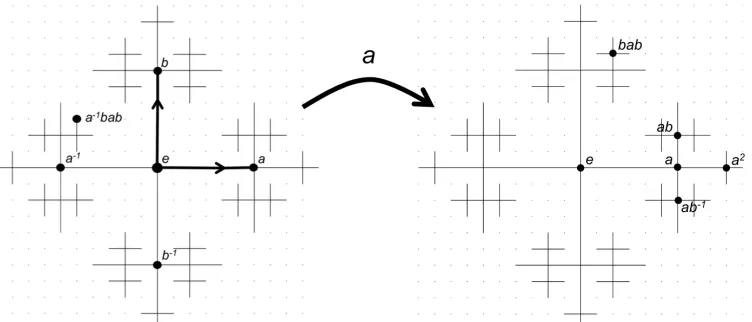
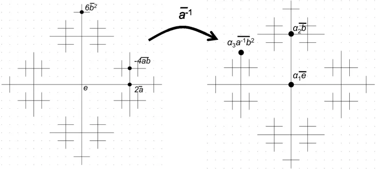
Figure 2.1: The …gure on the left shows the Cayley graph of F2, which F2 acts freely
upon. Several vertices labeled. The …gure on the right shows the image of these vertices under the action of a on the tree.
G. The groupG always acts freely upon its Cayley graph, and the vertices of are in one-to-one correpsondence with the elements of G. If G is a free group, and the generating set is a basis, then the Cayley Graph of G is a tree. In fact, we have the following well-known result, which will be important in the next chapter. The theorem may be found in [7], Theorem 3.20.
Theorem 2.4. If G is a group, thenG is free if and only if G acts freely on a tree.
Example 2.5. Let F2 = ha; bi be the free group on generators a and b. Then, F2
acts its Cayley graph , which is an in…nite tree. Part of is pictured in Figure 2.1. From any vertex v 2 V ( ), we see four edges leaving v. The upward vertical edge is identi…ed with the b, the generator of F2, and the downward edge with b 1.
Similarly, we identifyawith the horizontal edges leavingv in the rightward direction, and identifya 1 with the horizontal edge leaving the vertex in the leftward direction. In fact, in this tree we can identify every vertex of with some element of F2.
identi…ed with a, we obtain the vertex ea=a. Similarly, the vertex a 1 is obtained from moving from e to the left by one edge. If we travel upward from a 1, along a b edge, we obtain the vertex a 1b. Then, moving rightward along a, we obtain the
vertexa 1ba, and moving upward again transports us to the vertexa 1bab, as labeled
in Figure 2.1.
How does F2 act on ? Given some v 2V ( ), remember that we can identify v
with an element ofF2, call ith. Then, given somea 2F2, we de…ne the action ofaon
v byav =ah, whereah is the vertex of associated to the element ah 2F2. As an
example, given the vertex a 1bab, the action of a on this vertex results in the vertex
a(a 1bab) = bab. Geometrically, we may view the action as shifting the vertices of
to the right, as in Figure 2.1.
Once we de…ne the action ofF2 on the vertices of , the action of F2 on the edges
of is completely determined. The fact thatF2 acts freely on follows easily, when
we keep in mind that the vertices of are in one-to-one correspondence with the elements of F2.
2.3
Crossed Products
If Gis a group and D is a ring with identity, then the (ordinary) group ring D[G]
is formed by taking sums of the form Pg2Gqgg, where only …nitely many of the
qg 2 D are non-zero. Addition in the group ring is given in the obvious way, and
multiplication is given by
X
g2G
qgg
! X
h2G
rhh
!
=X
g2G
X
h2G
qgrhgh
!
whereghdenotes the product ofg withhinG. It is easy see that theD[G]is a ring with identity 1e, where 1 is the identity of D, and e is the identity of G. Typically, the multiplicative identity of D[G]is simply written as 1.
In studying group rings, other algebraic objects arise by altering the multiplication in the group ring. An algebraic structure arising in this manner is the crossed product, which is de…ned as follows. Suppose G is a group acting on a ring D so that there is a map : G ! Aut (D), which is not necessarily a homomorphism. Denote the automorphism (g) by g. LetG=fg :g 2Gg be a copy of G, which will be used
to de…ne multiplication in what follows. Then, we can form the crossed product D G by taking sums of the form Pg2Grgg, where only …nitely many of the rg are
non-zero. Addition is taken in the obvious way, and we can view D G as a free, left D-module with basisG. In order to make D Ga ring, multiplication in D G is de…ned using two unexpected rules:
1. (Skewing) For g 2G and r2D, we have gr= g(r)g.
2. (Twisting) If g; h 2 G, then gh = (g; h)gh, where gh denotes their product in D G, gh is the product inG, and (g; h) is some unit in D. Thus, when multiplying gh, the result di¤ers fromgh by some unit.
Using this de…nition, it is not apparent that multiplication in D Gis associative. In fact, additional assumptions must be imposed in order to guarantee the associa-tivity of D G, assumptions on the twisting function :G G! U(D), the units of D. For our purposes, however, D G will always constructed beginning with a group ring R[G], so that associativity will not be a concern.
possible to de…ne multiple crossed product structuresD G, with each crossed product essentially di¤erent. Therefore, to be precise, we would need to specify the skewing function and twisting whenever introducing a crossed product. However, this ambiguity rarely leads to confusion, and we often say “a crossed product D G” rather than “the crossed product D G” in order to emphasize this fact.
It is clear that every unit in D is a unit in D G. Does the same follow for the elements of G? That is, given some g 2G, is theg 2D Ginvertible? The answer is in the a¢ rmative. Before showing this, we need to …nd the multiplicative identity of D G. Our …rst thought is that 1e should be the identity. In fact, we have that for any x=Pg2Gqgg 2D G;
1e X
g2G
qgg
!
= X
g2G
1eqgg
= X
g2G
1 e(qg)eg
= X
g2G
qg (e; g)g.
following.
Proposition 2.6. If g 2 G, then g 2 D G is invertible, with g 1 =ug 1 for some
unit u2D.
Proof. One can verify that theg g1( (g; g 1))g 1 = 1e, and (g 1; g) 1g 1 g =
1e, so g is invertible on both sides. The associativity of D G asserts that the left and right inverse must be equal, so that 1
g ( (g; g 1)) = (g 1; g)
1
. Note that their common value is a unit inD.
If the skewing inD G is trivial, so that g 2Aut (D)is the identity function for
each g 2 G, D G is known as a twisted group ring, denoted by Dt[G]. When the twisting is trivial, so that (g; h) = 1 for each g; h2G, the crossed product is a skew group ring, denoted byDG. In the case of skew group rings,Gembeds into DG, so that we may remove the overbars and write elements of DGas Pg2Gqgg. If
both the skewing and twisting are trivial, thenD Gis justD[G], the ordinary group ring.1
Where would these objects arise in the study of group rings? The following construction can be found in [9], p. 2, and will be important in Chapter 5. Let R be a ring and G be a group, with N a subgroup. We wish to relate the group ring R[G] in some way to N and the collection of cosets G=N. Set H =G=N. Because H is a collection of cosets, to each coset x 2H …x some coset representative x2G, so that x = N x. Then, let H = fx:x2Hg G be the collection of all coset representatives. It follows thatGis the disjoint unionSx2HN x. Therefore,R[G]is the direct sum Px2HR[N]x, and every element of R[G] can be expressed uniquely in the form Px2Hfxx where fx 2 R[N]. This means that R[G] can be viewed as 1While there does not seem to be a consensus, the notation used here (Dt[G], DG, andD[G])
a free R[N]-module with basis H. If N C G, then H =G=N is a group. Setting D=R[N], the structure relatingR[G]with N and H is a crossed product D H.
To verify that multiplication in this structure is skewed and twisted, we begin by investigating the twisted multiplication of elements in H. Given x and y 2 H, we have N xN y =N xy. This means that xy 2 N xy, and therefore xy= nxy for some n 2 N, which is a unit in D. Beginning with elements of H and passing to their corresponding preimages in H, we then have a function : H H ! N U(D), where U(D) denotes the set of units in D. It follows that xy = (x; y)xy, which gives the twisting.
To study the skewing, note that because N / G, we have gDg 1 = D for each
g 2 G. Thus, every element of G induces an automorphism on D via conjugation. In particular, the elements of H induce an automorphism on D. This gives a map
: H ! Aut (D) de…ned by : x 7! x, where x is the automorphism that
conjugates by x. It follows that
xf = xf x 1 x
= x(f)x;
CHAPTER 3
D
F
-MODULES
3.1
Introduction
SupposeQis a …eld andF a …nitely-generated free group. In 1964, Paul Cohn proved that all …nitely-generated ideals in the group ring Q[F] are free as Q[F]-modules. Using this result, we may also deduce that …nitely-generated submodules of free Q[F]-modules are free. Cohn’s proof was technical and di¢ cult, using what he termed a “weak reduction algorithm.” In 1990, Hog-Angeloni proved the same result in [3], using the geometry of Q[F] to greatly simplify the arguments. This chapter generalizes these ideas to crossed products D F, with D a division ring and F a …nitely-generated free group.
By borrowing ideas from Hog-Angeloni, we o¤er a geometric interpretation for the elements ofD F. Using these geometric notions, we implement a method to reduce the collective “diameter” of collections of elements from D F. By doing this, we are able to prove that …nitely-generated submodules of free D F-modules are free.
It is worth noting that we are primarily interested inD F-modules in this chapter. For this reason, if M is aD F-module, then we use bold faced font for the elements x2 M to distinguish them from elements of D F (the “scalars”) and elements of F. This has the potential to be confusing when M = D F. In this case, we use bold font for the elements of D F that we consider to be in the module, and we do not bold the elements of D F that are “scalars.”
3.2
The Geometry of
D
F
In what follows, let D be a division ring, and F a …nitely-generated free group with identity e. If T is the Cayley graph ofF, then F acts freely onT, and T is a tree. Further, inT, there is a bijective correspondence between F and V (T), the vertices of T. Thus, we may view the elements of F as vertices inT, and vice versa.
In any tree , any two u; v 2 V ( ) have a unique reduced path de…ned between them. For what follows, we will use the termgeodesic to describe that path. This path includes a number of edges of , so we can de…ne the length of a path to be the number of edges in that path. We can measure the distance between two vertices u; v 2 V ( ) by calculating the length of the geodesic between the vertices. In addition, if w is the midpoint of an edge in T, then we can measure the distance betwen w and a vertex u by drawing a geodesic from w to u, and counting the half-edge traversed by taking w to its neighboring vertex as1=2 of an edge.
Figure 3.1: An illustration of Proposition 3.1.
Proposition 3.1. Suppose p; q; u; v are four distinct vertices or midpoints of edges in a tree . Let denote the geodesic between p and q, the geodesic betwen q and u, and the geodesic between u and v. Given that is disjoint from , and is disjoint from , consider the path from p to v obtained by following from p to q, then fromq to u, and …nally from u to v. This path is reduced, so that it is the unique geodesic from p to v.
Proof. Figure 3.1 gives a graphical intepretation for the hypotheses of the proposition. Suppose on the contrary that the path is not reduced. Because is disjoint from and , and all three of these paths are reduced. Because the path fromp tov is not reduced, it must be due to cancelling edges coming from and . It follows that and share an edge, and in addition, the paths share a vertex, call itz.
Beginning at the point q, we may follow until we come to the pointz. Then, we may take the path fromz tou, and …nally take fromuback to q. This produces a loop in the tree . Further, the loop may not fully reduce to a trivial path, because the geodesic is disjoint from and . Thus, we have a contradiction to the fact that is a tree, and the edge path from p to v; described in the statement of the proposition, must be reduced.
Choose some element x2D F. Then, x=Pg2F qgg, where only …nitely many
of the qg are non-zero. Geometrically, we can viewx as a …nite collection of vertices
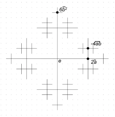
Figure 3.2: A geometric representation for x=2a 4ab+ 6b2 2D F.
vertices of T are identi…ed with the elements of F, the vertices included in x are those vertices g with qg 6= 0. The coe¢ cient assigned to each vertex is qg. The
summands qgg with qg 6= 0 will be called points of x. Alternatively, if qg 6= 0, we
might also refer to the vertexg as a point inx. Using this interpretation for elements of D F, we may viewD F as the set of all …nite collections of vertices in T, each with an assigned non-zero coe¢ cient inD.
Example 3.2. TakingDas the rationals, andF as the free group on two generators a and b, suppose x=2a 4ab+ 6b2. Figure 3.2 o¤ers the geometric interpretation
for x.
attain this maximal distance to the vertex e. Such points will be called extreme points of x.
The diameter of x, written diam (x), is the length of the longest geodesic from one point of xto another, where it is understood that the coe¢ cients assigned to the endpoints are non-zero. Under this de…nition, for any g 2G we have diam (qg) = 0, so the elements ofD F containing only one point have diameter 0: De…nediam (0)to be 1. We might also use the term diameter to refer to a reduced geodesic between points inxthat attains the lengthdiam (x). The de…nition of diameter also provides a notion of a radius forx, by de…ning the radius of xto bediam (x)=2.
Remark 3.3. Let us phrase these terms in a slightly more familiar context. If we let D = Q, and F = Z, then we may take D F to be the ordinary group ring
Q[Z]. Given some x 2 Q[Z], we have x=P1i= 1qiti, where only …nitely many qi
are non-zero. In fact, the ring Q[Z] is a Laurent polynomial ring. Then, points of x would be those terms qiti with qi 6= 0. The term dist (x) would be the maximum
of the set fjij:qi 6= 0g. Further, diam (x) would be maxfji jj:qi; qj 6= 0g, the
di¤erence between the highest and lowest degree terms ofx.
Example 3.4. Letxbe as in Example 3.2. Then,dist (x) = 2, because the maximal number of edge paths between a vertex in x and the vertex e is 2. In fact, 2 is the distance between ab and e, and it is also the distance between b2 and e. Therefore,
the points 4ab and 6b2 are extreme points of x. We also have that diam (x) = 4,
which is the distance between the verticesb2 andab. The reduced edge path between b2 and abis a diameter of x.
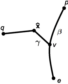
^
x, as the midpoint of the geodesic between two points in xwhose length attains the diameter ofx. If diam (x)is even, then^xis a vertex inT (whose assigned coe¢ cient might be zero). Ifdiam (x)is odd, then ^xis a midpoint of an edge in T. If uis the endpoint of a diameter with ^x as a midpoint, we call the geodesic joining ^x to u a radius of x. Note that the radius has length diam (x)=2.
Example 3.5. This continues Examples 3.2 and 3.4. Because the geodesic between b2 andabhas the vertexeas a midpoint, it follows thateis the barycenter ofx. That
is, ^x=e. Note that e is the barycenter of ^x, even though the coe¢ cient assigned to e by x 2D F is zero. Then, the geodesics joining e to b2 and e to ab are radii of
x, and they have length2 = diam (x)=2.
Given the de…nition of barycenter, it is not immediately clear that the barycenter of x is well-de…ned. Is it possible that x would contain two diameters with distinct midpoints? We prove this cannot happen by using the following propositions:
Proposition 3.6. Lety be the midpoint of a diameter of x. Supposeq is any vertex in the tree T, and let be the geodesic from q to y. If we set r= diam (x)=2, then there is some other point of x, call it p, so that: (1) The distance from p to y is r, and (2) The geodesic from p to y is disjoint from .
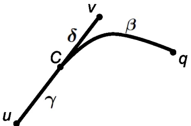
Figure 3.3: The relationship between the points and paths decribed in the proof of Proposition 3.6
Given some pointq ofx, consider the geodesic running betweenq andC. As leaves C, it cannot use the same edge as both and , because and are disjoint Without loss of generality, suppose that does not leaveC using the same edge as . Then, must be totally disjoint from , because if intersected at some point, the edge path beginning at C formed by following to the intersection with , and back toC would be a cycle in the treeT. Thus, and must be totally disjoint. By settingp=u, we are done.
An immediate consequence of this proposition that if q is a point of x, and C a midpoint of a diameter, then the distance from q to y must be no larger than
diam (x)=2. Otherwise, we could …nd some point p of x so that the geodesic from p to q is longer than diam (x), which contradicts the maximality of diam (x). We exploit this in the following proposition.
Proposition 3.7. If x2D F, then the barycenter of x is well-de…ned.
Proof. Suppose x contains two diameters, with respective midpoints w1 and w2.
Then,w1 and w2 are two possible candidates for the barycenter of x, and we want to
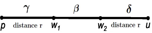
Figure 3.4: The relationship between the points described in the proof of Proposition 3.7.
Let denote the edge path between w1 and w2, and suppose the length of is
l >0. We want to arrive at a contradiction, and it will follow thatl = 0, sow1 =w2.
Using the Proposition 3.6 with C=w1 and q=w2, we can …nd some pointp so that
the distance fromw1 topisr, and the geodesic fromw1 top, call it , is disjoint from
. Applying the proposition again, this time with C = w2 and q =w1, we can …nd
some other point, call it u, so that the distance from w2 to u is r, and the geodesic
fromw2 tou, call it is disjoint from . See Figure 3.4 for an illustration.
The edge path from p to w1 is reduced and disjoint from . Further, the edge
path between w2 and u is reduced and disjoint from . It follows from Proposition
3.1 that the edge path from p to u obtained by traveling from p to w1 (distance r)
and then fromw1 tow2 via (distancel) and …nally from w2 tou (distancer) gives
a reduced edge path with length 2r+l > diam (x). This is a contradiction, and it follows that l= 0. Thus w1 =w2, and the barycenter is well-de…ned.
Given thatx^is well-de…ned, we prove the following result, which will be useful in the proof of several lemmas in Section 3.4.
Proposition 3.8. Ifpis an extreme point ofx, then the geodesic frompto the vertex e passes through x, and^ p is the endpoint of a diameter of x.
Figure 3.5: An illustration of the proof of Proposition 3.8.
consider the geodesic fromx^to e, it must intersect at some point (possibly only at e). Then, let v denote the point where these two geodesics intersect, and the edge path from ^xto v. If the length of is 0, then ^x lies on the edge path . Thus, we need to show that the length of is0.
Note that because of our choice ofv, the path obtained by following from^xtov, and then from v to pis reduced, and therefore, the geodesic from ^xto p. Because r is the length of any radius of x, the distance betwen ^x and p must be at most r. Because v lies on this geodesic, its distance from p must be at most r. Further, because the distance fromptoe iss, it follows that the distance fromv toe must be at least s r. By Proposition 3.6, we can …nd a point q of x so that the geodesic between q and ^x has length r, and is disjoint from the geodesic between p and x.^ Therefore, the path betweenq and ^xis disjoint from . See Figure 3.5.
the maximality of s. We conclude that the length of must be 0, so x^=v, and x^ lies on the geodesic , as desired.
What is the distance from x^ to e? If this distance were larger than s r, then using the same logic above, the distance from the point q toe would be larger than s. Thus, the distance from ^x to e is s r. Because the distance from p to e is s, and ^x lies on the geodesic betweenp and e, it follows that the distance from p to x^ is exactlyr. Then, the distance fromp toq is 2r = diam (x), p is the endpoint of a diameter of x.
The group F acts on T, and in particular, F acts on the vertices of T. Let x2D F. Because xis a can be viewed as a collection of vertices inT, so we obtain an action of F on x by letting F act on the vertices of x. Algebraically, for h 2 F and x=Pg2F qgg, we have
hx=X
g2F
h(qg) (h; g)hg
where h is some automorphism of D, and (h; g) is some invertible element of D.
Thus, we notice that the coe¢ cient associated to hg by hx is non-zero if and only if the coe¢ cient assigned to g byx is non-zero.
The vertexhgis simply the vertexg under the action ofh. Therefore, given some h 2 F, a geometric interpretation for hx can be obtained by letting h act on the vertices of x, and slightly altering the coe¢ cients at each resulting vertex. In fact, the vertices used in hx are precisely the collection of vertices obtained by letting h act on the vertices ofx.
diam hx = diam (x). In addition, it is also clear that the barycenters of xand hx satisfy the relationship hxc = h^x, where h^x is the action of h 2 F on the vertex or edge midpoint ^x.
Figure 3.6: A geometric interpretation for the action ofa 1 on x.
Example 3.9. This continues the previous examples. The action ofa 1 onxgives
a 1x=
a 1(2) a 1; a e a 1(4) a 1; ab b+ a 1(6) a 1; b2 ab2:
For simplicity, write a 1x as
1e+ 2b+ 3a 1b2. Then, by looking at Figure 3.6,
we see that the action of a 1 on x shifts vertices of x to the left, and changes the
coe¢ cients. Further, we observe that diam a 1x = diam (x) = 4, and that the
barycenter a[1xis a 1. Notice that this is the same as a 1^x, because^x=e.
3.3
Linear Combinations in
D
F
module) and 1; :::; n 2 D F (the ring). Then, consider the linear combination
Pn
i=1 ixi. By writing i =
P
g2Fqi;gg, we may rewrite the linear combination as
Pn i=1
P
g2Fqi;ggxi . Consider each summand qi;ggxi with qi;g 6= 0, and …nd the
summand(s) such that dist (qi;ggxi) is maximized. These summands will be called
extreme summands, because they are the summands with the maximal distance from the vertex e. Each extreme summand each contain at least one point qgg that
realizes this maximum distance. Call such points extreme points of the linear combination.
Remark 3.10. Let us try to phrase these terms in a more familiar context: the ring
Q[x]of polynomials in one variable over the rationals, which we view as aQ-module. Given a linear combination q1p1(x) + +qnpn(x), with qi 2 Q and pi 2 Q[x],
the analogue for extreme summands of the linear combination are thoseqipi(x) with
maximal degree. Then, the extreme points are the terms of eachqipi(x) that realize
this maximal degree.
3.4
D
F
-modules
Consider the leftD F-module J generated by the …nite collectionx1; :::xn 2J. We
writeM =hx1; :::;xni. We would like to replace this set with a linearly independent
set y1; :::;ym, withm n, so that hy1; :::;ymi =M. In this section, we present an
algorithm that allows us to do this.
First, we present an algorithm for …nitely-generated submodules of D F, which are simply ideals in D F. Given a collection x1; :::xn 2 D F, the algorithm
linearly independent. At that point, we may remove all zero elements to obtain a basis for …nitely-generated ideals inD F.
Our eventual goal is to prove that all …nitely-generated submodules of free D F -modules are free. By using the result in D F (which is free with rank 1), we may translate the result to modules with higher rank. Because we will eventually work in free modules with rank larger than 1, it will be useful to introduce matrices into our discussion.
Given an m n matrix M, with entries in D F, each row of M corresponds to an elements of the module (D F)n. Then, we de…ne the row space of M to be the submodule of(D F)n generated by the rows of M. We also have the following de…nition.
De…nition 3.11. An n matrixA, with entries in D F, is called an elementary matrix if A is either then n identity matrix In, orA may be obtained fromIn in
one of the following ways:
1. A is obtained by interchanging two rows of In.
2. A is obtained by multiplying one row of In by a unit.
3. Ais obtained by changing one o¤-diagonal entry ofInfrom a0to some non-zero
element of D F.
Under these requirements, it is easy to see that the elementary matrices are invertible matrices, and generate a group under multiplication. Let En(D F)
denote the group of n n matrices generated by the elementary matrices.
Left-multiplication by elements of En(D F) preserves the row space of a given
Proposition 3.12. Let A2 Em(D F) and M be an m n matrix with entries in
D F. If J is the row space ofM, then the row space of of AM is alsoJ.
Proof. Let x1; :::;xm 2 (D F)n denote the rows of M. Then, J = hx1; :::;xmi.
It su¢ ces to show that if A is an elementary m m matrix, then the rows of AM generate J, because every element of Em(D F) is a …nite product of elementary
matrices.
IfAis an elementary matrix, thenAhas one of the three forms given in De…nition 3.11. For the …rst two forms, it is obvious that the rows of AM also generate the moduleJ, so suppose thatAhas the third form. Then, Ais identical to the identity matrix, except for having some r 2 D F in some non-diagonal entry, say the k-th row and the l-th column. If y1; :::;ym denote the rows of AM, then we have the
relationship yi = xi for i 6= k, and yk = xk+rxl. In this case, though, it is clear
that hy1; :::;ymi=hx1; :::;xmi, and the result follows.
With the de…nition of elementary matrices and this proposition in hand, we are prepared to prove the following result.
Theorem 3.13. Given a linearly dependent collection x1; :::;xn 2D F, with each
xi 6= 0, there exists y1; :::;yn 2D F and a matrixA2En(D F) so that
A 2 6 6 6 6 4 x1 .. . xn 3 7 7 7 7 5 = 2 6 6 6 6 4 y1 .. . yn 3 7 7 7 7 5,
and Pni=1diam (yi)<
Pn
i=1diam (xi).
The proof of the theorem is long and involved, so it will be broken into smaller pieces. First, we set up the proof: because x1; :::;xn are linearly dependent, there
exists 1; :::; n 2 D F, not all zero, such that Pin=1 ixi = 0. Writing i =
P
g2Fqi;gg, we may rewrite the linear combination as
Pn i=1
P
g2F qi;ggxi . For
what follows, we only consider summands with qi;g 6= 0. Moreover, because we care
about the geometry of this situation, and not the coe¢ cientsqi;g (except that they are
non-zero), we will omit qi;g from our discussion. Consider the set of extreme points
of the linear combination (those points of maximal distance from the identity vertex e) and extreme summands (those gxi with qi;g 6= 0 containing an extreme point of
the linear combination). Set s as the distance from extreme points of the linear combination to the vertex e. Of the extreme summands, choose one with maximal diameter. Without loss of generality, we will call thishxk, for someh2F and a …xed
k 2 f1; :::; ng. Set r = diam hxk =2. This means that the greatest distance any
point ofhxk may have from the barycenterhxdk isr. Among the extreme summands,
let R be the set of those summands that contain an extreme point p, such that the geodesic from p to the vertex e passes through hxdk, the barycenter of hxk. Such
extreme points with this property will be called special extreme points, and R is the collection of summands containing special extreme points.
The proof of the theorem proceeds with the following lemmas.
Lemma 3.14. The extreme summand hxk is in the collection R, and the distance
from hxdk to the vertex e is s r. Further, every special extreme point is at distance
r fromhxdk.
Proof. In order to show that hxk is inR, we show that any extreme point of hxk is
shows that the geodesic from p to e passes through hxdk, and p is a special extreme
point. Becausehxk contains a special extreme point, it is a member of the collection
R.
Furthermore, in the proof of Proposition 3.8, we showed that p must be the endpoint of a diameter of hxk, so the distance between p and hxdk is r. Because
the geodesic between p and e passes through hxdk, it follows that the distance from
d
hxk to e is s r. From this, we may conclude that the distance from any special
extreme point to hxdk is r.
Lemma 3.15. Ifpis any extreme point of somegxi 2 R, thenpis special. Moreover,
if gxi 2 R, and r0 = diam (gxi)=2, then the distance from gxci to hxdk isr r0.
Proof. Notice that, due to our choice of r = diam hxk =2, we must have r r0.
Because gxi 2 R, it follows that gxi has a special extreme point, call it q. Then,
Proposition 3.8 shows that the geodesic fromqtoemust pass throughgxci. Moreover,
q is the endpoint of a diameter in gxi, its distance from gxi is r0. From these two
facts, it follows that the distance from gxci is s r0.
Because q is special, the geodesic from q toe must also pass through hxdk. Note
that the distance from q togxci isr0, and the distance from q tohxdk is r (by Lemma
3.14). Thus, starting at qand moving to the vertexe, we …rst pass throughgxci, and
then throughhxdk. This shows thathxdk lies on the geodesic betweengxci and e, and
using the fact that the distance from hxdk to e is s r, it follows that the distance
between hxdk and gxci isr r0.
Letpbe any extreme point ofgxci. Then, the geodesic fromptoepasses through
c
gxi. After passing through gxci, our work above shows that the geodesic must also
Lemma 3.16. If q is any point of some gxi 2 R, then the distance fromq to hxdk is
at most r.
Proof. Letr0 = diam (gx
i)=2. Lemma 3.15 shows that the distance from gxci to hxdk
is r r0. If q is any point of some gx
i, its distance to dgxk must be at most r0.
Because the distance fromgxci tohxdk isr r0, it follows that the distance from q to
d
hxk is at most r.
Lemma 3.17. The extreme summand hxk is the only copy of xk appearing in R.
That is, if gxk2 R, then g =h.
Consider the subtree of T formed by taking all vertices with distance at most r away from hxdk. Note that any diameter of this subtree must have midpoint hxdk,
using the same arguments to show that the barycenter is well-de…ned (Proposition 3.7). By Lemma 3.16, every gxi 2 R must be contained in this subtree. Moreover,
if anygxi 2 R has diameter2r, then it must be true that gxci =hxdk. Suppose that
there is some g 2F so thatgxk 2 R. Then, because the action of g on xk preserves
the diameter ofxk, we have
diam (gxk) = diam (xk) = diam hxk = 2r.
Thus, gxdk = hxdk. This implies that g^xk = h^xk (see the remarks on p. 23), and
h 1g^xk=^xk. Thus, the action ofh 1g onx^k is trivial. However, because the action
of F on T is free, we have h 1g =e, and g =h. An important consequence of this is that
X
gxi2R
qi;ggxi =qk;hhxk+
X
gxi2R,i6=k
qi;ggxi:
Lemma 3.18. The summands in R satisfydiam Pgx
i2Rqi;ggxi <diam (xk):
Proof. The sumPgx
i2Rqi;ggxi is formed by taking a collection of summands from the
linear combinationPni=1 ixi = 0. Furthermore, the de…nition of R is the collection
of all summands containing special extreme points. Because Pni=1 ixi = 0 and R
contains all special extreme points, the coe¢ cients of all special extreme points must vanish in the sumPgxi2Rqi;ggxi. For simplicity, set w=
P
gxi2Rqi;ggxi.
Once again, consider the subtree formed in the proof of Lemma 3.17. The element w is contained in the subtree, because every summand in the de…nition of w is con-tained in the subtree. We want to show that diam (w)<diam (xk) = 2r. Suppose
on the contrary that this were not the case. Then, we would havediam (w) = 2r, and the barycenterw^ would behxdk(by arguments in the proof of Lemma 3.17). Consider
a geodesic between two points of w with the length of as 2r. Note that, by the de…nition of diameter, if we view the endpoints of as points ofw, the coe¢ ecients on the endpoints must be non-zero. We will show that one of the endpoints must have distancesfrom the vertexe, so the endpoint is an extreme point. By 3.15, this point must be a special extreme point, which contradicts the fact that the coe¢ cient assigned to special extreme points must vanish in w.
Because hxdk is the barycenter of w, it must be the midpoint of , so that the
distance from hxdk to the endpoints is r. Futhermore, the radii extending from hxdk
to the endpoints of are disjoint, so at least one of these radii must be disjoint from the edge path from hxdk to e. Call the end of this radius u. Then, traveling from u
to hxdk (distance r), and then traveling to e (distance s r) show that the distance
We are now ready to prove Theorem 3.13:
Proof. For 1 k n, de…ne yk = Pgxi2Rqi;ggxi, and yi = xi for i 6= k. Note
that it is possible to have yk = 0. Clearly, Pdiam (yi) < Pdiam (xi), because
diam (yk)<diam (xk), and diam (yi) = diam (xi) for i6=k.
In the sum de…ning yk, we may pull the xk term out, as in the proof of Lemma
3.17. Then, collecting all terms in the sum using the same xi, we can write
yk=qk;hhxk+
X
i2f1;:::;ng
i6=k
fixi
for somefi 2D F. Then, form then n matrixA in the following way. For every
1 i n, i6=k, let thei-th row of A have a 1 on the diagonal, a zero in every other entry. For the k-th row, put fi in the i-th column, where i 6= k, and qk;hh in the
k-column. It follows that A x1 xn
T
= y1 yn
T
. It is not di¢ cult to see that the matrixA is generated by elementary matrices, soA2En(D F). This
completes the proof.
Repeated applications of Theorem 3.13 can take a linearly dependent generating set, and transform it into a generating set whose non-zero elements are linearly independent. We prove this in the following theorem.
Theorem 3.19. If x1; :::;xn 2 D F, then there exists y1; :::;yn 2 D F and a
matrix B 2En(D F) so that
and the collection of non-zero yi are linearly independent.
Again, by Proposition 3.12, the statement also implies thathx1; :::;xni=hy1; :::;yni.
Proof. We prove the result via the following inductively-de…ned algorithm, which begins with a collectionx1; :::;xn. In order to track of the iterations of our algorithm,
we will relabel each xi with the index x0;i. Each step of the algorithm will increase
the …rst index value by 1.
Step 1. Given the collection x0;1;x0;2:::;x0;n, if the non-zero elements of this collection
are linearly independent over D F, then we set yi =x0;i for each 1 i n,
and take B to be the identityn n matrix, and we are done. In particular, if x0;1 = x0;2 = =x0;n = 0, then we are done. Otherwise, let x0;1; :::;x0;k be
the non-zero elements of the collection (if need be, relabel), with k n. By Theorem 3.13, because the non-zero x0;1; :::;x0;k are linearly dependent, there
existsx1;1; :::;x1;k 2D F and a matrix A2Ek(D F) such that
A x0;1 x0;k
T
= x1;1 x1;k
T
andPki=1diam (x1;i)<
Pk
i=1diam (x0;i). We can expand Ato ann n matrix
A1 2En(D F), by adding rows and columns so that a 1 occurs in the diagonal
of the new rows and columns, and zeros everywhere else. For k < i n, we setx1;i= 0 (=x0;i, by assumption) and we have the equation
A1 x0;1 x0;n
T
= x1;1 x1;n
T
n
X
i=1
diam (x1;i)< n
X
i=1
diam (x0;i).
The next step is de…ned inductively. After completing the …rst j steps, we have a matrix Aj 2En(D F), so that
Aj x0;1 x0;n T
= xj;1 xj:n
T
; (3.1)
wherexj;1; :::;xj;n 2D F are such thatPni=1diam (xj;i)<Pni=1diam (xj 1;i). Then,
thej+ 1-th step is:
Step j+ 1. Given the collection xj;1; :::;xj;n, we may permute thexj;i so that the non-zero
elements of the collection occur at the beginning of the list. This permuation of thexj;i must also be accompanied by permuting thatn rows ofAj in the same
manner, so we maintain the relationship given in Equation (3.1) Then, after permuting, suppose thatxj;1; :::;xj;r are the non-zero elements of the collection,
where r n. If xj;1; :::;xj;r are linearly independent, we can set yi = xj;i for
eachi, and andB =Aj, and halt the algorithm. Otherwise, by Theorem 3.13,
there existsxj+1;1; :::;xj+1;r 2D F and a matrixA 2Er(D F) so that
A xj;1 x0;r
T
= xj+1;1 xj+1;r
T
andPri=1diam (xj+1;i)<
Pr
i=1diam (xj;i). Then, we can expandAto an n n
matrix A0 2 En(D F), by adding rows and columns that are 1 only on the
diagonal ofA0, and zero everywhere else. Forr < i n, set xj+1;i =xj;i (= 0,
A0 xj;1 xj;n
T
= xj+1;1 xj+1;n
T
,
where Pni=1diam (xj+1;i) <
Pn
i=1diam (xj+1;i). De…ne the matrix Aj+1 2
En(D F) asA0Aj. Then,
Aj+1 x0;1 x0:n
T
= xj+1;1 xj+1;n T
.
We proceed to the next step of the algorithm.
The claim is that this algorithm must eventually halt. To justify the claim, notice that for any step j, Pni=1diam (xj;i) is bounded below by n, in which case
diam (xj;i) = 1 for each i, and xj;i = 0. Because the sum of the diameters of the
generators is …nite, strictly decreasing after each step, the algorithm must halt.
We are now ready to present the main result from the chapter:
Theorem 3.20. Suppose thatDis division ring withF a …nitely-generated free group. If N is a …nitely-generated submodule of a freeD F-moduleJ, then N is also a free module.
If the non-zero elements of the …rst column of M are not linearly independent, then 3.19 says that we can …nd some A1 2 Em(D F) so that the non-zero entries
of the …rst column of A1M is linearly independent. If the non-zero entries of the
second column of A1M are not linearly independent, we can …nd a matrixA2 so that
the non-zero entries of the second column of A2A1M are linearly independent.
Our concern at this point is that, while the non-zero entries of the …rst column of A1M are linearly independent, is this also true for the non-zero entries of the
…rst row of A2A1M? In fact, this is the case. By multiplying on the left by
A2 2Em(D F), we are essentially performing row operations on the matrix A1M.
Thus, the entries of the …rst column ofA2A1M are linear combinations of the entries
of the …rst column ofA1M. Because the non-zero entries of the …rst column ofA1M
are linearly independent, this must also be true ofA2A1M.
We continue this process of multiplying by matrices from Em(D F) to ensure
that the non-zero entries of each column column are linearly independent. If we do this for each of then columns, we obtain a matrixM0 =A
nAn 1 A1M, so that for
each …xed column ofM0, the non-zero entries of that column are linearly independent. Because M0 is obtained from M by elementary matrices, it follows from Proposition 3.12 that the rows of M0 generate the sameD F-module as the rows ofM, which is the module J.
M0 = 2 6 6 6 6 6 6 6 6 6 6 4 .. . 3 7 7 7 7 7 7 7 7 7 7 5
where represents the …rst non-zero entry of a given row. Because the non-zero entries of each column are linearly independent, it follows that the rows of M0 are linearly independent, and form a basis forJ. Thus, J is a free module.
The following is an easy corollary. Recall that a right zero divisor is an element x2D F, x6= 0, so that there is some non-zero a2D F with ax= 0.
Corollary 3.21. D F is a domain.
CHAPTER 4
ORE LOCALIZATION
4.1
Introduction
Suppose k is a division ring, andG a group. If we could embed the ordinary group ringk[G]into a division ringQ, then all modules overQwould be free. In particular, submodules of freeQ-modules would be free. Sometimes it is not necessary to invert every element of k[G] in order to ensure that …nitely-generated submodules of free modules are free. For example, in the group ringQ[F], withF a …nitely free group, submodules of free Q[F]-modules are free, even though Q[F] clearly has elements that are not units.
If G is a group of the form HoF, then our work on p. 11 shows that the group ring k[G] can be viewed as a crossed product k[H] F. If we can embed k[G] into a larger ring Q so that the elements ofk[H] are invertible, then it seems reasonable that this resulting structure would have the formD F, where Dis a ring containing the multiplicative inverses of k[H]. In the previous chapter, we proved that D F satis…es the property that all …nitely-generated submodules of freeD F-modules are free. Thus, if M is a …nitely-generated submodule of a free k[G]-module, then M has a basis when viewed as module overD F.
elements of S are invertible when mapped into Q? A special case for this problem comes from taking S = R f0g, in which case Q would be a division ring (and because R ! Q is an embedding, R must be a domain). The process of creating inverses for the elements of a ring R is called localization. If S R; and we wish to only construct inverses for the elements of S, then this process is referred to as the localization of R at S. In this chapter, we present the theory of Ore localization, which o¤ers the most intuitive way to localize R atS.
Ring theorists often study localization in a more general setting. By not requiring that the map R ! Q to be an embedding, a ring theorist also does not need the assumption that the elements ofS do not divide zero inR. However, because we are primarily interested in embeddings, we do assume that S contains no zero divisors.
The theory contained in this chapter can be found in many texts on localization and noncommutative rings. References include [12] and [4].
4.2
Conditions to Localize
R
at
S
Given a ring R with some subset S, we wish to construct a ring Q and a map ' : R ! Q so that for each s 2 S, the element '(s) 2 Q is invertible. Further, wish the map' to be an embedding, so that we can viewR Q. The most obvious way to construct Q is to mimic the construction of the rationals from the integers. Thus, we will construct Qfrom “fractions”with elements ofR in the numerator and elements of S in the denominator.
this notation is ambiguous because ab could mean b 1a or a 1b. In the commutative setting, this makes little di¤erence, but because R might not be commutative (and thereforeQmight not be commutative), we must specify which “side”of the fraction should contain the denominator. Because it seems more intuitive to write the denominator on the right, as ina=b=ab 1, we will write our fractions in this manner,
although we could do the following construction with denominators on the left in a similar manner. We now turn our attention to …nding conditions on R and S that guarantee that such a ring Q exists.
What must be true of S if such a ring Q exists? An element r 2R is said to be regularif it is not a zero divisor. If there were somes2S which divides zero in R, then it is clear that mapR !Qcannot be an embedding. Thus, every element ofS must be regular. Further, we must guarantee that 02= S to avoid trying to invert 0. In addition, we need12S, so that every element ofR can embed intoQvia the map r 7!r1 1. Lastly, the product of invertible elements in Q needs to be invertible, so
S should be multiplicatively closed. A set S that satis…es these conditions is called a multiplicative1 subset of R. We now give a de…nition for our ringQ.
De…nition 4.1. LetR be a ring withS a multiplicative subset of R. Suppose that a ringQexists, along with an embedding ' :R !Q, so that every element ofQ can be written in the form '(a)'(b) 1, with a 2 R and b 2 S. Then, Q is called the right ring of fractions for R with respect toS. The ring Q is usually written as RS 1.
Given this de…nition, it is not immediately clear that the right ring of fractions is unique in anyway. Is it possible for there to be two right rings of fractions forR with
1In the more general theory, the de…nition of multiplicative sets does not include the assumption
respect to S, say Q and Q0, which are not isomorphic? The following propositions, the …rst of which may be found in [12], can be used to show that this may not occur.
Proposition 4.2. Let R be a ring withS a multiplicative subset, so that a right ring of fractions exists with respect to S, call the ring of fractions Q. Further, suppose that ' : R ! Q is an embedding. Then, whenever there is a ring homomorphism
: R ! Q0 such that (s) is invertible in Q for every s 2 S, there exists a unique homomorphism :RS 1
!Q such that ' = .
Proof. Givena2Rand b2S, de…ne :Q!Q0 by '(a)'(b) 1 = (a) (b) 1. We need to show that is well-de…ned on the elements of Q. To show this, suppose that '(a)'(b) 1 ='(r)'(s) 1. Then, we have the following equation in R:
'(a)'(s) = '(r)'(b)
'(as) = '(rb).
Beause' is an embedding, it follows that
as =rb.
From this, we conclude that
(as) = (rb)
(a) (s) = (r) (b)
(a) (b) 1 = (r) (s) 1
Thus, is well-de…ned. It is also not di¢ cult to show that is a homomorphism. Further, the fact that '= and that also follows quickly.
Proposition 4.3. Suppose Q and Q0 are both right rings of fractions for R with respect to S, with embeddings ' : R ! Q and : R ! Q0. Then, there is an isomorphism between Q and Q0.
Proof. The previous proposition gives us a unique map : Q ! Q0, which is a homomorphism, so that ' = . Reversing the roles of Q and Q0, we also obtain a unique map 0 :Q0 !Q, where 0 ='. Then, we have the equations
0 ' = '
0 = .
Thus, 0 : Q ! Q. By the previous proposition (taking Q0 = Q), 0 is the unique homomorphism so that( 0 ) ' ='. Becauseid
Q is another such function,
we have that idQ = 0 . Similarly, idQ0 = 0, and it follows that and 0 are
the desired isomorphisms.
In light of this proposition, every right ring of fractions forR with respect to S is essentially the same. For this reason, we can say “the right ring of fractions”rather than “a right ring of fractions,” and use the notation RS 1 to denote this ring with no ambiguity.
Given S a multiplicative subset of R, we wish to construct the ring RS 1. We
is right permutable if and only if for every s 2 S and r 2 R, there existst 2 S and x2R such thatsx=rt. Thus, right permutability can be viewed as a weak version of commutativity, because it allows us to take an element of S and an element of R, and …nd a common multiple. Notice that right permutability is trivially satis…ed if R is a commutative.
A similar notion can be de…ned for left permutability2, although it is not true that left and right permutability are equivalent in general settings. We will see in the next chapter that left and right permutability are equivalent in group rings, though. IfS is a right permutable, multiplicative subset ofR, thenS is sometimes called a right denominator setinR. The following well-known thereom justi…es this term, and gives necessary and su¢ cient conditions for the existence ofRS 1. The proof of
this theorem (without making the assumption that the elements of S are regular in R) may be found in [12].
Theorem 4.4. Suppose that R is a ring with S a multiplicative subset of R Then, the right ring of fractions RS 1 exists if and only if S is right permutable.
Proof. As this is an “if and only if” statement, we need to prove two directions. (RS 1 exists implies right permutable) To prove this direction, if RS 1 exists,
pick any s2S and r 2R. Then, by the de…nition of RS 1, the product s 1r must
have the formab 1 for some a
2R and b2S. By clearing denominators, we obtain
s 1r = ab 1 rb = sa.
This shows that S is right permutable.
2The left permutability replacesrS
(Right permutable implies RS 1 exists) We prove this direction by de…ning an equivalence relation on R S, and then de…ning operations on R S= to make this set form a ring.
When considering elements ofR S, we view the …rst coordinate as the numerators and the second as the denominators of the fractions we wish to form. Then, de…ne a relation on R S by(r; s) (p; q) if there exists x; y 2R such that sx; qy 2S and (rx; sx) = (py; qy), where equality means that the …rst coordinates are equal, and the second coordinates are equal. Essentially, the de…nition of means that we can regard two “fractions” as the same under if they can be brought to the same denominator, and after bringing them to the same denominator, the numerators are also equal.
We can show that is an equivalence relation. Re‡exivity and symmetry of are trivial, so we will only prove transitivity. Suppose that (r; s) (p; q) and
(p; q) (a; b). Then, there exists x1; y1; x2; y2 2 R such that sx1; qy1; qx2; by2 2 S
and (rx1; sx1) = (py1; qy1), (px2; qx2) = (ay2; by2). Because S is right permutable,
there exists c 2 R and d 2 S such that (qy1)c = (qx2)d 2 S. Because q 2 S, and
elements of q are not zero divisors, we cancel theq’s to obtainy1c=x2d. Then,
(rx1c; sx1c) = (py1c; qy1c)
= (px2d; qx2d)
= (ay2d; by2d).
This shows that (r; s) (a; b), and is an equivalence relation. Then, consider the collection of equivalence classes R S= . Looking toward our end goal, we denote R S= by RS 1, and write the equivalence class associated to (a; b)
a=b2RS 1. An important observation is that, by the de…nition of , ifa=b 2RS 1 and c2R is such thatbc2S, then a=b= (ac)=(bc).
We de…ne addition on RS 1 as follows:
r=s+p=q = (rc+pd)=u
where u = sc = qd 2 S, for some c 2 R and d 2 S. We can …nd such a u by the right permutability of S. Essentially, to add two elements of RS 1, we bring them to a common denominator and then add the numerators. Multiplication is de…ned inRS 1 by:
r=s p=q = (rd)=(qc)
wherec2Sandd2Rsatisfysd =pc, and the existence of suchcanddis guaranteed by the right permutability ofS. The motivation for this de…nition makes more sense if we proceed through some intermediate steps. Suppose thatsd =pc. Momentarily ignoring the fact that sd; pc might not be inS, we have
r=s p=q = (rd)=(sd) (pc)=(qc)
= (rd)=(pc) (pc)=(qc)
Then, because pc occurs in the denominator of the …rst fraction and the numerator of the second, we can “cancel” it to obtain
r=s p=q = (rd)=(qc)
well-de…ned on the equivalence classes ofRS 1. Further, equipped with these operations, RS 1 forms a ring with additive identity0=1, and multiplicative identity1=1.
If we de…ne a map ':R!RS 1 by' :r
7!r=1, then' is easily veri…ed to be a ring homomorphism. Furthermore, ifr=1 = 0=1, then there is somex; y 2R so that
1x= 1y2S (sox2S), and (rx; x) = (0; y), where equality is taken inR S. Thus, rx= 02R, and because x2S, which does not contain zero divisors, it follows that r= 0. This shows that the map 'is an embedding, and we can view R as a subring of RS 1 by identifying elements of R with their image under'.
If we view S RS 1, then every s
2 S can be written s = s=1. Using the de…nition of multiplication onS R= , we haves=1 1=s= 1=1 = 1=s s=1, so every element of S is invertible in RS 1. Additionally, every element RS 1 has the form ab 1 fora 2R and b2S.
We have shown that the ring RS 1 is a right ring of fractions for the ring R with
respect to S, and it follows that the right ring of fractions exists. Further, every right ring of fractions is isomorphic toRS 1 as above.
brought to a common, non-zero multiple by multiplying on the right, as shown in the following proposition.
Proposition 4.5. If R is a right Ore domain, given a …nite collection of non-zero r1; :::; rn 2R, there exists non-zero s1; :::; sn2R, such that r1s1 =r2s2 = =rnsn.
Proof. The proof will be by induction on n. For n = 2, this is just the right Ore condition on R. Then, we assume that any collection of n non-zero elements of R can be brought to a common multiple, and consider the collection of non-zero r1; :::; rn; rn+1 2 R. By assumption, there exists non-zero t1; :::; tn 2 R so that
r1t1 = = rntn. Denote their common value by u. Then, u 6= 0. Because R
satis…es the Ore condition, there exists non-zero s and s0 2 R so that us = r
n+1s0.
Then, r1t1s =r2t2s = =rntns = rn+1s0. By writing si = tis for 1 i n, and
sn+1 =s0, the proof is complete.
Besides Ore domains, another special case of Theorem 4.4 is the case where S =
R , the regular elements of R. In this case, the ring RS 1 is called the right
classical ring of quotients for R. This ring has the interesting property that every element is either a zero divisor or a unit.
4.3
Some Examples and Properties of Ore Localization
At this point, while we have necessary and su¢ cient conditions for the existence of the ringRS 1, we do not have any examples of ringsR with multiplicative subsetsS
As another example, if we take R to be a division ring and S a multiplicative subset, S is easily veri…ed to be right permutable, so RS 1 exists. We can also see that R is a right ring of fractions for itself, so Proposition 4.3 shows RS 1 is
isomorphic toR.
The following proposition shows that if R contains ideals that are free with rank larger than 1, thenR is not an Ore domain.
Proposition 4.6. Let R be a right Ore domain. Then, a right ideal I 6= f0g in R is a free right R-module if and only if it is principal.
Proof. Suppose that I is a free, right R-module. If the rank of I were larger than one, pick two distinct basis elements from I, call them x and y. Note that x and y must both be non-zero. Because R is a right Ore domain, there exists non-zero s; t2Rso thatxs =yt. Then,xs yt= 0, andxandyare not linearly independent. This is a contradiction, and it follows that the rank of I cannot be larger than one. Thus,I is principal.
If I is non-zero, right, principal ideal in the domain R, then it is clear that the generator for I serves as a basis for I as a rightR-module. Thus, I is free.
The following proposition shows that Ore domains are common in the study of ring theory.
Proposition 4.7. If R is a right Noetherian domain, then R is a right Ore domain.
right ideals, and deduce that R is not right Noetherian. For n 0, de…ne the right ideal In=xR+yxR+y2xR+ +ynxR. Then, we have the ascending chain
I0 I1 :
The claim is that In (In+1 for everyn, so the chain does not stabilize. If this were
not case, let n be the smallest natural number for which In =In+1. It follows that
yn+1x
2In, and we can write
yn+1x=
n
X
i=0
yixai
where not everyai = 0. Letr be the smallest natural number so thatar6= 0, so that
ar 2S. Note that r < n+ 1. Then, because we are in a domain, we can cancel ayr
from both sides to obtain:
yn+1 rx =
n
X
i=r
yi rxai
yn+1 rx = xar+ n
X
i=r+1
yi rxai
yn+1 rx
n
X
i=r+1
yi rxai = xar
y yn rx
n
X
i=r+1
yi r 1xai
!
= xar.
This contradicts the assumption that x and y are such that xR\yR =f0g, and it follows that In (In+1 for every n. Thus, R is not Noetherian.
implies the following:
Proposition 4.8. If R is a right Artinian domain, then R is a right Ore domain.