DEMOGRAPHIC RESEARCH
VOLUME 34, ARTICLE 10, PAGES 285
−
320
PUBLISHED 12 FEBRUARY 2016
http://www.demographic-research.org/Volumes/Vol34/10/ DOI: 10.4054/DemRes.2016.34.10
Research Article
Childhood socioeconomic status, adult
socioeconomic status, and old-age health
trajectories:
Connecting early, middle, and late life
Zachary Zimmer
Heidi A. Hanson
Ken R. Smith
©2016 Zachary Zimmer, Heidi A. Hanson & Ken R. Smith.
This open-access work is published under the terms of the Creative Commons Attribution NonCommercial License 2.0 Germany, which permits use, reproduction & distribution in any medium for non-commercial purposes, provided the original author(s) and source are given credit.
1 Introduction 286
2 Data and methods 288
2.1 Sample 288
2.2 Measurement 289
2.3 Two-step analytic strategy 291
3 Findings 294
3.1 Childhood and adult SES 294
3.2 Morbidity trajectories and survival probabilities 295 3.3 Modeling group membership by childhood and adult SES 303
3.4 Changes in SES and group membership 305
4 Discussion 307
5 Acknowledgements 311
Childhood socioeconomic status, adult socioeconomic status, and
old-age health trajectories:
Connecting early, middle, and late life
Zachary Zimmer1
Heidi A. Hanson2
Ken R. Smith3
Abstract
BACKGROUND
The paper advances literature on earlier-life socioeconomic status (SES) and later-life health in a number of ways, including conceptualizing later-life health as a developmental process and relying on objective rather than retrospective reports of childhood and adult SES and health.
METHODS
Data are from the Utah Population Database (N=75,019), which contains variables from Medicare claims, birth and death certificates, and genealogical records. The morbidity measure uses the Charlson Comorbidity Index. SES is based on converting occupation to Nam-Powers scores and then dividing these scores into quartiles plus farmers. Analyses are conducted in two steps. Group-based trajectory modeling estimates patterns of morbidity and survival and divides the sample into sex-specific groups ordered from least to most healthy. Multilevel ordered logistic regression incorporating Heckman selection predicts group trajectory membership by SES in adulthood conditioned upon childhood SES.
RESULTS
Higher SES in childhood is associated with membership in groups that have more favorable morbidity trajectories and survival probabilities. SES in adulthood has additive impact, especially for females. For example, if a female is characterized as being in the lowest SES quartile during childhood, her probability of having the most favorable health trajectory improves from 0.12 to 0.17 as her adult SES increases from the lowest to highest quartile.
1 University of California, San Francisco, U.S.A. E-Mail: [email protected]. 2 University of Utah, Utah, U.S.A.
CONCLUSIONS
Results suggest both childhood and adult SES independently impact upon old-age health trajectories.
1. Introduction
The current study uses a large population database linking information from over 75,000 persons across early, middle, and late life to establish how the combination of childhood and adult SES are associated with late-life long-term morbidity patterns. Socioeconomic status has long been seen as a crucial morbidity and mortality determinant (Adler et al. 2008; Antonovsky 1967; Bobak et al. 2000; Braveman et al. 2010; Chen, Yang, and Liu 2010; Hay 1988; Hayward et al. 2000; Kadushin 1964; Mackenbach et al. 2008; Marmot et al. 1991). The topic of SES and health has attracted growing attention in the United States, particularly as population health has improved overall while social class gradients in health have steepened (Elo 2009; White and Preston 1996). In an attempt to explain these divergent trends, research has focused on pathways that account for persistence in and expansion of health inequalities. Some of these include mediators such as stress, social support, and preventive as well as risk behaviors (Engdahl and Tambs 2010; House et al. 1990; Marmot and Siegrist 2004; Petrelli et al. 2006; Tang, Chen, and Krewski 2003).
autonomously important and combines to create a net effect on later-life health. Finally, there is the social mobility model (Hallqvist et al. 2004). Social mobility contends that SES in adulthood can mitigate or reverse effects of early life. For instance, upward mobility might moderate or even reverse somewhat the negative impacts of low early-life SES. Similarly, SES disadvantages later in early-life can outweigh benefits that might have been accrued due to earlier life advantages. Except for the critical period model, these arguments all suggest that someone born into a low SES family is not destined to endure poor health in late life, but rather that the health effects of early-life SES are malleable (Pudrovska and Anikputa 2014).
The current study adds to the discourse in a number of ways. Testing for both childhood and adult SES effects requires measures that are consistent over generations and able to reflect relative transitions in status that take place across the life course. This study employs a broad SES indicator that is consistently and reliably measured across early and later life and allows for an assessment of relative SES position within generations. While most studies of early-life SES rely on retrospective information, the current study uses objective information obtained from vital and administrative records.
Studies have consistently demonstrated an association between SES and mortality or morbidity, although few have examined effects of SES on morbidity as it develops and changes over the course of old age. An exception is Haas (2008), who examined functional health trajectories in Health and Retirement Study data. The current study examines comorbidity outcomes using objective data obtained by employing Medicare information spanning an 18-year period. By asking whether childhood and adult SES affects patterns of late-life health measured over the long-term, this analysis aims to assess how a combination of early-life and mid-life characteristics might have lasting influences on the aging experience. Morbidity is conceptualized using an index that summarizes nearly all serious illnesses afflicting older individuals (Charlson et al. 1987). Some older persons will have no or few chronic health conditions across all ages while others will accumulate conditions over time. The study employs a two-step modeling approach that first identifies a discrete set of groups. These groups consist of persons that have similar comorbidity trajectories. These trajectories also incorporate mortality probabilities within the modeling. Incorporating rather than excluding mortality means that the end of life is considered as part of a developmental process of old-age health (Haviland, Jones, and Nagin 2011).
(Adler et al. 2008; Macintyre 1997; Marmot et al. 1991). Elo (2009), in an extensive review of divergent measures of SES and their impact on health, notes that occupation has the advantage of being related to both income and education and of summarizing a combination of social, environmental, and economic characteristics that are relevant for health outcomes. The current study converts occupations into Nam-Powers Occupational Status Scores (Nam and Terrie 1982), which themselves are derived in a way that represents educational requirements and income levels that relate to specific occupations.
In sum, the current analysis adds to the discourse on childhood and adult SES and late-life health in a number of ways. It uses data that allows for reliable comparisons of SES across generations. Conceptualizing late-life health as a developmental process that includes both morbidity and mortality, it considers the impact of earlier life characteristics on old-age health as a process. By using Nam-Powers SES scores it converts occupation into a multifaceted indicator of SES. Finally, using a database linking population information across sources, it relies on objective rather than retrospective reports of health and SES in both childhood and adulthood.
2. Data and methods
2.1 Sample
Age-based Medicare eligibility begins at age 65, but individuals in this study are observed starting at 66, resolving the problem that those who become eligible during the calendar year when they turn 65 are only partially observed for that year. Observation ends at age 105 due to virtually no observations beyond that age. Those in the data were eligible for Medicare in 1992 when records become available, or became eligible between 1993 and 2009. There are 499,974 such CMS enrollees. However, two criteria were imposed that reduced the initial sample for analysis. First, to become part of the sample individuals must be Utah residents with sufficient family history information to link them genealogically and reliably into the UPDB. Many of those with CMS records could not be linked to their Utah-based parents and therefore lack childhood SES measures. About 45% of persons in these CMS records are individuals born outside Utah. Second, omitted from the sample are those enrolled in Medicare Advantage. These individuals appear in the Medicare records but are covered by an alternate form of insurance and do not have medical encounters billed to Medicare during the time they are on Medicare Advantage. Overall, individuals excluded from the initial sample are: 209,172 not linked to a parental death certificate; 49,111 linked to a parental death certificate but the information on parental occupation is not retrievable; 42 with poor data quality; 77,613 part of the Part C Advantage Enrollment; and 13,998 not observed for multiple years and thus lacking sufficient information to establish trajectories. The analytical sample therefore comprises150,038 long-term Utah residents with sufficient information on which to conduct trajectory modeling.
The trajectory modeling used in this study is computationally intensive. To enable the models to converge we used a 50% random selection, providing a final sample size of 75,019. Once an individual is included in the sample, the only additional form of attrition is mortality. The reliability of the 50% sample was tested by repeating the 50% sample selection two additional times with commensurate re-analysis of data. Each replicate resulted in nearly identical results.
Each subject is observed annually from 1992, or the year they turn 66, until death or until 2009. Doctor visits are combined during the course of a year into one observation per person per year to create a person-year file. The maximum number of yearly observations per person is 18, one for each year of coverage between 1992 and 2009. The selected sample generated 713,935 person-year observations, or about 9.5 years per individual.
2.2 Measurement
Certificates. Annual morbidity measures reflect a count of conditions reported in the Medicare data and listed in the Charlson Comorbidity Index (CCI) (Charlson et al. 1987). The CCI has been employed in numerous studies and has been deemed to be among the most valid measures of comorbidity (Huntley et al. 2012). Conditions comprising the CCI are: myocardial infarction, congestive heart failure, peripheral vascular disease, cerebrovascular disease, dementia, chronic pulmonary disease, rheumatologic disease, peptic ulcer disease, mild liver disease, diabetes (mild to moderate), diabetes with chronic complications, hemiplegia or paraplegia, renal (kidney) disease, any malignancy, moderate/severe liver disease, metastatic solid tumor, and HIV/AIDS.
Childhood and adult SES are based on occupations converted into Nam Powers Occupational Status Scores (NP-SES) (Nam and Powers 1968; Nam and Powers 1983). NP-SESs range from 1 to 100 for specific occupations, with scores based on educational requirements and income levels typical for people with that occupation (Nam and Terrie 1982). Therefore these scores do more than measure occupation: they are a broad indicator of SES. The measure has been used in numerous studies linking SES and health (e.g., Meyer et al. 2004; Steenland et al. 2003; Steenland, Hu, and Walker 2004; Temby and Smith 2013).
Different data sources provide us with information about childhood and adult SES. A person’s childhood SES is measured using information about the usual occupation of his/her parent as listed on the parent’s death certificate. If there is information on more than one parent, which is not a common occurrence since the majority of mothers are listed as housewives, the measure reflects the highest NP-SES of the individual’s deceased parents – most often the father. Indeed, in only about one in five cases is there an occupation for mother and only in a very small minority of these cases does the mother’s occupation result in the higher NP-SES score. A comparable measure for adult SES is derived from information about occupation noted on a birth certificate where the subject appears as a parent. Multiparous individuals can have more than one occupation recorded. We rely on a measure that is the highest SES score across all births for each father-mother pair named on a birth certificate. We note that there are cases where occupation changes across different instances of childbirth, but in the vast majority of cases they do not vary greatly. Moreover, sensitivity analyses that considered SES to be based on the average or the lowest scores across instances did not alter the findings.
The remaining individuals are sorted into quartiles based on the generation-specific NP-SES distributions.
Models that link childhood and adult SES to later-life health adjust for early- and mid-life confounders that are available in the UPDB and have been shown to be associated with both SES and later-life health outcomes (Smith et al. 2009). Number of children of the subject is included. Increasing parity may increase risk of later-life comorbidity through physiological pathways, particularly among females, who disproportionately bear physiological and psychological costs of childbirth and childrearing (Kirkwood and Rose 1991). Next is number of siblings of the subject. Increasing sibship size relates to the way in which resources get shared, while greater sibship size has been shown to lower educational attainment and lead to unhealthy lifestyle choices (Behrman and Taubman 1986; Hart and Smith 2003). Activity level within the Church of Jesus Christ of Latter-day Saints (LDS or Mormons), the predominant religion in the state of Utah, is measured as: active, inactive, and non-LDS. Membership in the LDS church has been shown to favorably influence health through behavioral, social network, and support mechanisms (Koenig 2013; Mineau, Smith, and Bean 2004). Indicators of timing of key family transitions are included in the models. Early age of parental death can affect available resources while growing up and therefore negatively affect SES attainment, while also serving as a risk factor for one’s own health through a series of potential genetic and social influences (Smith et al. 2009). Also controlled is whether a parent dies before age 12 of the individual. Since own occupation is measured when the individual bore a child, the age at which the subject’s child was born may be consequential. Younger age of birth could limit attaining a stable labor market position. Later age at birth may be related to health, with those able to bear children at advanced reproductive ages having better health (Smith and Hanson Forthcoming). Therefore, estimated models include the age of the individual at the time at which the indexed child is born (i.e., the birth certificate that reflects SES in adulthood). Finally, race (white versus non-white), which has long been shown to be associated with both SES and health outcomes, is adjusted for.
2.3 Two-step analytic strategy
1999; Nagin and Tremblay 2001; Roeder, Lynch, and Nagin 1999; Zimmer et al. 2014; Zimmer et al. 2012). The number of groups into which the sample is separated is based on criteria that combines Bayesian Information Criteria (BIC), post-estimation posterior probabilities, and subjective examination of groups that pragmatically distinguish health patterns (Nagin 2005). Trajectory groups are formed as a function of number of CCIs at a given age, coupled with chances of surviving from one age to the next. CCIs are modeled using a Poisson distribution with quadratic functions, which are suitable given that age patterns in CCI are non-linear. The probability of dying at a given age is modeled simultaneously (Haviland, Jones, and Nagin 2011; Zimmer et al. 2012). Patterns of morbidity and mortality risks are sex-specific.
2. Estimating association of childhood and adult SES with group membership: A regression procedure estimates the association between childhood and adult SES and trajectory group membership. GBT modeling produces for each subject post-estimation probabilities of the chance of belonging to each group. These probabilities add to 1.0 for each individual. Each subject is assigned to the group for which they have the highest probability. The average highest probability is an indicator of model fit. The recommendation consistently followed in the literature (Dodge, Shen, and Ganguli 2008; Nagin 2005; Zimmer et al. 2014) is that an average highest posterior probability of 0.80 for each group is an indicator of good model fit. For these data the average for each group is greater than 0.80 with an overall average being 0.85. However, it is possible that some individuals are misclassified. For instance, some will have highest posterior probabilities of under 0.50. For our data, only 5% of the female sample and 6% of the male has a highest posterior probability of under 0.50. Moreover, as is widely appreciated, the misclassification of persons in a given trajectory generally makes the findings more conservative, especially - as we suggest is the likely scenario - when the misclassification is random. Such misclassification means that some people will be placed in a trajectory incorrectly, a situation that serves to minimize differences between the two trajectories in question. Further, to assure unbiased standard errors in the regression procedure that follows the classification, regression weights are constructed to be equal to posterior probabilities. This means that the more confident we are of group membership, the higher will be the weight given to that observation.
correction variable based on the Inverse Mills Ratios (IMR), derived from a probit model where the dependent variable measures whether the individual was retained for the substantive analysis or not. Including the IMR as a covariate in the regressions predicting group membership assesses and corrects for potential nonrandom sample selection induced by the missing data (Heckman 1976). The variables used for the selection part of the estimation include age in 1992, birthplace (UT vs. outside of UT), median family income from the county of residence based on the 1990 Census, county-level population from the 1990 Census, and affiliation with the LDS church (active, inactive, non-member).
The first step of the analysis, the trajectory group modeling, indicated that subjects break into discrete groups that can be classified from most to least healthy. Individuals in less healthy groups have higher CCIs at any age and are less likely to survive. Since these groups are ordered and represent the dependent variable, we use sex-specific ordered logit regressions to estimate the probability of group membership, ordering groups from least to most healthy (lowest value to highest value in the ordered scale).
Given the UPDB, we know whether individuals within the data are siblings. These sibsets mean the assumption of statistical independence is violated. The method used for adjusting for this is a mixed modeling approach that includes random effects at the sibling level (Raudenbush and Bryk 2002). To estimate an ordered logit model with random effects the Generalized Linear Latent Mixed Models (gllamm) procedure is employed (Rabe-Hesketh and Skrondal 2008). Gllamm provides coefficients for individual level effects, like childhood and adult NP-SES, and a variance and standard error of variation for within-family (sibling) random effects.
Several models are tested. The first includes only childhood SES and the IMR. The second adds adult SES. The third adds additional covariates. Interactions between childhood and adult SES were tested, but these did not statistically improve model fit and therefore childhood and adulthood were deemed to be independent predictors of health outcomes. For parsimony, interaction models are not shown.
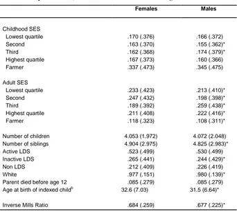
Descriptive statistics for model covariates are provided in Table 1. Table 1 also indicates whether distributions significantly differ across females and males. While all 75,019 observations are part of the first stage Heckman selection model, the second stage includes those with complete occupational information, a sample size of 39,338.
Table 1: Descriptive statistics showing means (standard deviations in parentheses) for covariates in the ordered regression modela
Females Males
Childhood SES
Lowest quartile .170 (.376) .166 (.372)
Second .163 (.370) .155 (.362)*
Third .162 (.368) .174 (.379)*
Highest quartile .167 (.373) .160 (.366)
Farmer .337 (.473) .345 (.475)
Adult SES
Lowest quartile .233 (.423) .213 (.410)*
Second .247 (.432) .198 (.398)*
Third .189 (.392) .259 (.438)*
Highest quartile .211 (.408) .222 (.416)*
Farmer .118 (.323) .108 (.311)*
Number of children 4.053 (1.972) 4.072 (2.048)
Number of siblings 4.904 (2.975) 4.825 (2.983)*
Active LDS .523 (.499) .530 (.499)
Inactive LDS .265 (.441) .244 (.429)*
Non LDS .212 (.409) .226 (.419)
White .977 (.151) .980 (.139)*
Parent died before age 12 .085 (.279) .085 (.279)
Age at birth of indexed childb 32.6 (7.03) 31.5 (6.64)*
Inverse Mills Ratio .684 (.259) .677 (.225)*
Note: a
Descriptive statistics based on sample with complete occupation information (N= 20,687 for females and 18,651 for males). b The indexed child is the child whose birth certificate provides the information for SES. * Difference between males and females significant at p< .05.
3. Findings
3.1 Childhood and adult SES
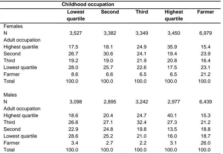
adult SES in a higher quartile. Quartiles are based on generation-specific NP-SES scores. Since occupational distributions changed over the course of a generation, the same occupation, with the same NP-SES score, could fall into a different SES quartile for childhood versus adulthood measures. Downward mobility is also noticeable. For those with farming as their childhood SES there is considerable movement to other categories. Only 21.2% of females and 26.0% of males whose childhood SES classification is ‘farmer’ are categorized as farmers as adults
Table 2: Distribution of adult SES by childhood SES and sexa
Childhood occupation Lowest
quartile
Second Third Highest
quartile
Farmer
Females
N 3,527 3,382 3,349 3,450 6,979
Adult occupation
Highest quartile 17.5 18.1 24.9 35.9 15.4
Second 26.7 30.6 24.1 19.4 23.9
Third 19.2 19.0 21.9 20.8 16.4
Lowest quartile 28.0 25.7 22.6 17.5 23.1
Farmer 8.6 6.6 6.5 6.5 21.2
Total 100.0 100.0 100.0 100.0 100.0
Males
N 3,098 2,895 3,242 2,977 6,439
Adult occupation
Highest quartile 18.6 20.4 24.7 40.1 15.3
Third 26.6 27.1 32.4 27.3 21.2
Second 22.9 24.8 19.8 13.5 18.8
Lowest quartile 28.6 25.2 21.0 16.0 18.7
Farmer 3.4 2.7 2.2 3.1 26.0
Total 100.0 100.0 100.0 100.0 100.0
Note: a
Does not include cases with missing parental or own occupation.
3.2 Morbidity trajectories and survival probabilities
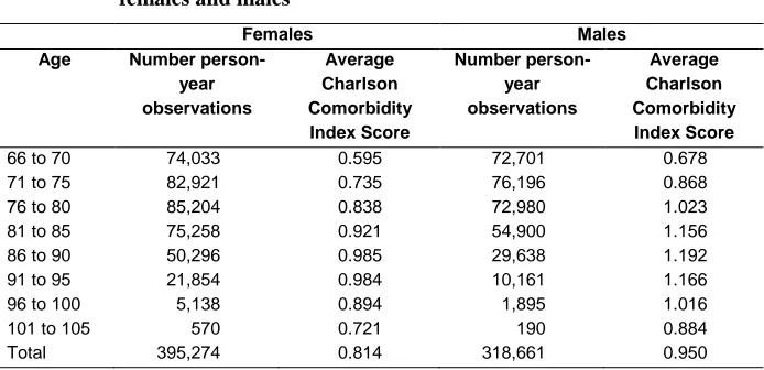
group until age 86–90, after which there is a decline. This drop is likely a function of mortality selection in that individuals living at advanced ages are less likely than others to be characterized by health problems detected by the CCI. Males have significantly higher average CCIs than females of the same age. This is consistent with research on sex differences in the conditions measured in the CCI and with higher male mortality (Schiller et al. 2012).
Table 3: Average Charlson Comorbidity Index Scores by age group for females and males
Females Males
Age Number
person-year observations
Average Charlson Comorbidity Index Score
Number person-year observations
Average Charlson Comorbidity Index Score
66 to 70 74,033 0.595 72,701 0.678
71 to 75 82,921 0.735 76,196 0.868
76 to 80 85,204 0.838 72,980 1.023
81 to 85 75,258 0.921 54,900 1.156
86 to 90 50,296 0.985 29,638 1.192
91 to 95 21,854 0.984 10,161 1.166
96 to 100 5,138 0.894 1,895 1.016
101 to 105 570 0.721 190 0.884
Total 395,274 0.814 318,661 0.950
Note: All differences in average CCI between males and females significant at p< .05.
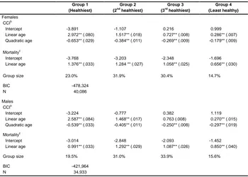
Table 4: Maximum likelihood parameter estimates for Charlson Comorbidity Index Score trajectories and drop-out due to mortality for females and males (standard errors in parentheses)a
Group 1 (Healthiest) Group 2 (2nd healthiest) Group 3 (3rd healthiest) Group 4 (Least healthy) Females CCIb
Intercept -3.891 -1.107 0.216 0.999
Linear age 2.972** (.080) 1.517** (.018) 0.727** (.008) 0.286** (.007)
Quadratic age -0.653** (.029) -0.384** (.011) -0.269** (.009) -0.179** (.009)
Mortalityc
Intercept -3.768 -3.203 -2.348 -1.696
Linear age 1.376** (.033) 1.284 ** (.027) 1.058** (.025) 0.656** (.030)
Group size 23.0% 31.9% 30.4% 14.7%
BIC -478,324
N 40,086
Males CCIb
Intercept -3.224 -0.777 0.382 1.119
Linear age 2.587** (.084) 1.468** (.017) 0.763 (.008) 0.270** (.015)
Quadratic age -0.539** (.033) -0.405** (.011) -0.250** (.008) -0.297** (.019)
Mortalityc
Intercept -3.014 -2.848 -2.093 -1.452
Linear age 0.991** (.033) 1.292** (.029) 1.087** (.026) 0.850** (.040)
Group size 19.5% 31.0% 33.9% 15.6%
BIC -421,964
N 34,933
Note: ** p < .01 * .01 < p < .05.
a
To assist in model convergence, age is scaled by subtracting the sample mean age and dividing the result by 10.
b
Poisson distribution.
c
Logit distribution.
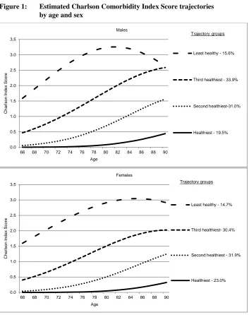
Figure 1 plots estimated CCIs by age. The four groups are distinct and ordered by increasing levels of morbidity. To facilitate interpretation, the groups are labeled simply from ‘healthiest’ to ‘least healthy’. CCI is plotted to age 90, since most point estimates beyond this age are based on a small number of surviving individuals. For instance, the entire group classified as least healthy died out by age 90 and therefore estimates beyond this age are not reasonable.
age 66, which increases to 3.0 by age 80, then levels off or and even declines at oldest ages. The decline at very old ages is likely a function of selectivity wherein the healthiest members of specific groups are the ones most likely to survive. All groups, if plotted out to older ages, would reveal a leveling-off then a decline in predicted CCI. Males display similar patterns, as do females with higher levels of CCI and an earlier peak for the least healthy group. As for the proportion that fit into each trajectory, for females and males alike the extreme CCI groups contain the smallest percentage of the sample: about 15% to 20%. The middle two trajectory groups contain slightly more than 30% each.
Figure 1: Estimated Charlson Comorbidity Index Score trajectories by age and sex
0.0 0.5 1.0 1.5 2.0 2.5 3.0 3.5
66 68 70 72 74 76 78 80 82 84 86 88 90
C
har
ls
on I
ndex
S
c
or
e
Age
Males
Least healthy - 15.6%
Third healthiest - 33.9%
Second healthiest-31.0%
Healthiest - 19.5% Trajectorygroups
0.0 0.5 1.0 1.5 2.0 2.5 3.0 3.5
66 68 70 72 74 76 78 80 82 84 86 88 90
C
har
ls
on I
ndex
S
c
or
e
Age
Females
Least healthy - 14.7%
Third healthiest- 30.4%
Second healthiest - 31.9%
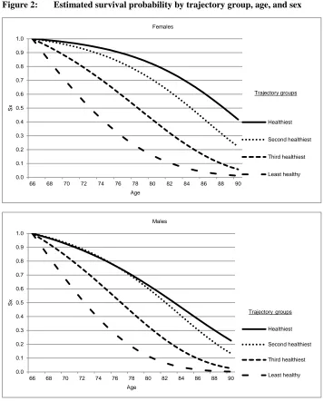
Figure 2: Estimated survival probability by trajectory group, age, and sex
0.0 0.1 0.2 0.3 0.4 0.5 0.6 0.7 0.8 0.9 1.0
66 68 70 72 74 76 78 80 82 84 86 88 90
Sx
Age
Females
Healthiest
Second healthiest
Third healthiest
Least healthy Trajectory groups
0.0 0.1 0.2 0.3 0.4 0.5 0.6 0.7 0.8 0.9 1.0
66 68 70 72 74 76 78 80 82 84 86 88 90
Sx
Age Males
Healthiest
Second healthiest
Third healthiest
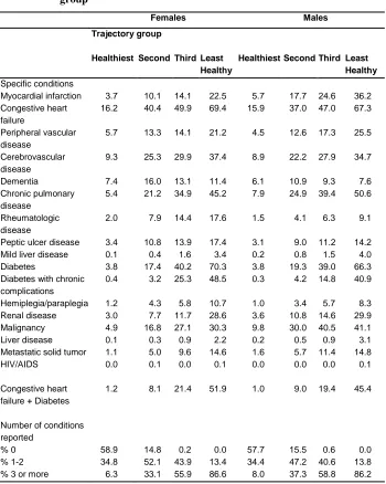
Deconstructing the CCI into its specific conditions provides an opportunity to assess if individuals in different trajectory groups are more or less likely to have specific conditions. Table 5 shows the percentage of individuals in each group that ever have specific conditions across the observation period, from 1992 to 2009, and the percentage that ever report no, one, two, three, or more of these conditions. Those in less healthy groups are much more likely to report almost any specific condition at some point, in that the percentage reporting conditions increases as trajectory group moves from most to least healthy. However, the difference is particularly acute for certain conditions. For instance, while the majority of females and males in the least healthy group have reported diabetes (70.3% females; 66.3% males), very few are diabetic in the healthiest group (3.8% females and males). An interesting comorbidity combination is congestive heart failure plus diabetes. Almost none of those in the healthiest group have both of these conditions (1.2% females; 1.0% males). This percentage increases across trajectory groups, with those in the least healthy group being about forty times more likely than those in the healthiest group to report the combination of these conditions (51.9% females; 45.4% males). Interestingly, the only condition that does not increase monotonically by trajectory group is dementia.
Table 5: Percentage that report specific conditions and the distribution of number of conditions reported, from 1992 to 2009, by trajectory group
Females Males
Trajectory group
Healthiest Second Third Least Healthy
Healthiest Second Third Least Healthy Specific conditions
Myocardial infarction 3.7 10.1 14.1 22.5 5.7 17.7 24.6 36.2
Congestive heart failure
16.2 40.4 49.9 69.4 15.9 37.0 47.0 67.3
Peripheral vascular disease
5.7 13.3 14.1 21.2 4.5 12.6 17.3 25.5
Cerebrovascular disease
9.3 25.3 29.9 37.4 8.9 22.2 27.9 34.7
Dementia 7.4 16.0 13.1 11.4 6.1 10.9 9.3 7.6
Chronic pulmonary disease
5.4 21.2 34.9 45.2 7.9 24.9 39.4 50.6
Rheumatologic disease
2.0 7.9 14.4 17.6 1.5 4.1 6.3 9.1
Peptic ulcer disease 3.4 10.8 13.9 17.4 3.1 9.0 11.2 14.2
Mild liver disease 0.1 0.4 1.6 3.4 0.2 0.8 1.5 4.0
Diabetes 3.8 17.4 40.2 70.3 3.8 19.3 39.0 66.3
Diabetes with chronic complications
0.4 3.2 25.3 48.5 0.3 4.2 14.8 40.9
Hemiplegia/paraplegia 1.2 4.3 5.8 10.7 1.0 3.4 5.7 8.3
Renal disease 3.0 7.7 11.7 28.6 3.6 10.8 14.6 29.9
Malignancy 4.9 16.8 27.1 30.3 9.8 30.0 40.5 41.1
Liver disease 0.1 0.3 0.9 2.2 0.2 0.5 0.9 3.1
Metastatic solid tumor 1.1 5.0 9.6 14.6 1.6 5.7 11.4 14.8
HIV/AIDS 0.0 0.1 0.0 0.1 0.0 0.0 0.0 0.1
Congestive heart failure + Diabetes
1.2 8.1 21.4 51.9 1.0 9.0 19.4 45.4
Number of conditions reported
% 0 58.9 14.8 0.2 0.0 57.7 15.5 0.6 0.0
% 1-2 34.8 52.1 43.9 13.4 34.4 47.2 40.6 13.8
3.3 Modeling group membership by childhood and adult SES
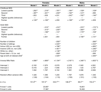
Table 6 presents parameters predicting group membership. A positive coefficient means that higher values for that variable are associated with a higher probability of being in increasingly healthy groups. Table entries are log odds. For instance, in Model 1 for females the estimated log of the odds for those in the lowest quartile is -.292. This means that in comparison to those whose childhood SES is in the highest quartile, those in the lowest have lower log odds of being in a healthier group. Exponentiation of the log odds (e-.292=.747) indicates that the odds that a female in the lowest quartile of childhood SES is in a healthier trajectory group relative to her counterpart in the highest quartile are lower by a factor of .747; or the lower-quartile female has about 25% lower odds than the highest-quartile female of being in a healthier group. Therefore, being in the lowest quartile of childhood SES translates into poorer health and lower survival probabilities. In general, coefficients for childhood SES below the highest quartile are negative, indicating a disadvantage of being in an SES category lower than the highest. For females, being in the lowest and second lowest groups is disadvantageous in comparison to the highest (coefficients of -.292 and -.397 respectively), while for males, being in the lowest, second, and third lowest groups are unfavorable in comparison to the highest (coefficients of -.184, -.192 and -.242 respectively).
Table 6: Ordered logit model predicting trajectory group membership, showing log oddsa
Females Males
Model 1 Model 2 Model 3 Model 1 Model 2 Model 3
Childhood SES
Lowest quartile -.292** -.218** -.181** -.184** -.109^ -.109^
Second -.397** -.321** -.249** -.192** -.121^ -.090
Third -.053 -.009 +.031 -.242** -.192** -.146**
Highest quartile (reference) --- --- --- --- --- ---
Farmer +.128** +.166** +.059 +.198** +.178** +.009
Adult SES
Lowest quartile -.515** -.410** -.370** -.172**†
Second -.313** -.230** -.309** -.127*
Third -.188** -.131* -.179** -.109*
Highest quartile (reference) --- --- --- ---
Farmer +.001 -.054 +.156** +.131*
Number of children -.058** -.066**
Number of siblings +.025** +.034**
Active LDS (vs. non LDS) +.796** +.683**
Inactive LDS (vs. non LDS) +.451** +.346**
White (vs. other) +.138** +.316**
Parent died < 12 (vs. not) -.090^ -.095
Age at birth of indexed childd +.025** +.055**
Inverse Mills Ratio +.896** +.889** +1.194** +.318**† +.348**† +.693**†
Intercept 1 -2.160 -1.970 -3.579 -2.079 -1.940 -4.561
Intercept 2 -0.416 -.224 -1.846 -0.243 -.120 -2.767
Intercept 3 1.592 1.787 0.152 1.991 2.096 -0.582
Random effect variance (SE) 1.426 (.126) 1.395 (.124) 1.200 (.115) 1.787 (.155) 1.679 (.151) 1.340 (.135)
Δ -2 LL 151.8b
** 157.2c
* 533.7c
** 106.0b
** 99.3c
** 744.2c
**
N level 1 units 20,687 18,651
N level 2 units 17,987 16,462
Note: ** p < .01 * .01 < p < .05 ^ .05 < p < .10.
a
Groups ordered from least healthy (lowest) to most healthy (highest).
b
Compared to model with intercept and Inverse Mills Ratio only.
c
Compared to previous model.
d
After adding other covariates, effects of both childhood and adult SES remain robust for females. The effect of adult SES is strong and significant for males, while some of the childhood SES coefficients for males are reduced to near- or non-significant levels. Nonetheless, on balance, for both males and females both childhood and adult SES affect health in old age. There is generally an important distinction between those in the highest childhood SES quartile versus others and highest adult SES versus others.
While coefficients are generally significant and in the expected direction for both sexes, there are differences by sex. Coefficients are by and large more robust for females across both childhood and adult SES, indicating that old-age morbidity trajectories of females appear to be more impacted by SES. We conducted statistical tests to determine if the male and female coefficients are different from each other and found that generally the differences are not large enough to be significant. There is a notable exception. The effect of adult SES being in the lowest quartile for females (-.410; p<.01) is significantly more negative than the equivalent effect for males (-.172; p< .01).
Being a farmer in adulthood is advantageous for males. Childhood SES of farmer is not significant for either females or males, and farmer SES in adulthood is not significant for females.
Most of the remaining covariates in Model 3 are significant. Those with healthier trajectories have lower parity, more siblings, are active and inactive LDS, are of white race, and have higher age at birth of the indexed child. A parental death before age 12 is moderately significant for females, decreasing the probability of being in a healthier trajectory.
The IMR is associated with being in a healthier trajectory, which indicates that the characteristics that determine sample selection are also related to health, and thus substantiates the two-stage Heckman strategy and concerns over sample selection. Estimates of random effects for all models are significant, suggesting strong sibling-specific heterogeneity acting upon group membership.
3.4 Changes in SES and group membership
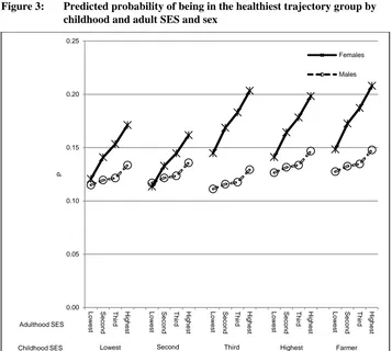
added on the far right. The graph is organized such that slopes indicate the probability of being in a particular trajectory group when moving from lowest to highest adult SES conditional upon childhood SES.
Figure 3: Predicted probability of being in the healthiest trajectory group by childhood and adult SES and sex
For both females and males, moving from lower to higher quartiles of SES increases the probability of being in the healthiest trajectory group in old age. However, the effect is much stronger for females, as clearly shown by steeper slopes. For example, conditional on a female’s childhood SES being in the lowest quartile, as adult SES increases from the lowest to highest the chances of being in the healthiest trajectory group rise from about 0.12 to 0.17. Conditional on a female’s childhood SES being in the highest quartile, the slope for being in the healthiest trajectory rises from
0.00 0.05 0.10 0.15 0.20 0.25 Low es t S ec ond T hi rd H ighes t Low es t S ec ond T hi rd H ighes t Low es t S ec ond T hi rd H ighes t Low es t S ec ond T hi rd H ighes t Low es t S ec ond T hi rd H ighes t P Females Males Adulthood SES
about 0.14 to 0.20. By contrast, if a male has lowest childhood SES, as adult SES increases from the lowest to the highest quartile the chances of being in the healthiest trajectory group rise from about 0.12 to 0.14, and conditional on a male’s childhood SES being in the highest quartile, the slope rises from about 0.13 to 0.15. Childhood occupation of farming provides an intriguing finding. For both females and males the probability of being in the healthiest group is greatest when childhood SES is ‘farmer’ and adult SES is in the highest quartile.
4. Discussion
The current study links childhood SES, indicated by occupation of parent, with adult SES, indicated by occupation at time of birth of children, and associates the combination of these with long-term developmental patterns in old-age health. A group-based trajectory (GBT) modeling approach was used to cluster individuals into those that experience more and less healthy morbidity and survival patterns in old age, with morbidity operationalized according to the Charlson Comorbidity Index or CCI (Charlson et al. 1987). This modeling approach indicated four trajectory groups conforming to an ordinal pattern of long-term health. The healthiest group, among both females and males, are individuals likely to survive to old age and experience virtually no morbidity conditions as they age from 66 onward. The least healthy group has much lower survival probabilities, has one or more condition at age 66, and experiences a rising number of conditions with increasing age. Deconstruction of the CCI indicated that the least healthy group is very likely to have a combination of congestive heart failure and diabetes in addition to other conditions, while those in the healthier groups are unlikely to have this mix of conditions.
noticeable, is not typically statistically significant in the models, except for one exception: the effect of lowest adult SES is statistically more robust for females.
The study adds to our understanding of earlier-life SES and later-life health in several ways. Using linked databases, the study was able to connect life-course characteristics in an objective way that avoided the need for retrospective information. By using a population database, the study was able to incorporate a large amount of data measuring decades of the life course in two generations. It suggested robust associations for SES measured similarly across generations. Importantly, by considering 18 years of Medicare information stretching from 1992 to 2009 the analysis has shown that the connection between earlier-life experiences and late-life health extends to long-term patterns that influence individuals as they age.
The ability to navigate the health care system is likely to vary by SES. If high SES individuals are better able to access the system and are more likely to seek medical care, then they are more likely to appear in Medicare records and therefore are more likely to be seen in the data. If this is the case, high SES individuals may very well be more likely to have morbidity conditions recorded, and our findings would represent a conservative estimate of the effects of SES on long-term health.
Sex differences are not always statistically significant yet appeared quite clear in the predicted probabilities shown in Figure 3, with stronger slopes for females. Past findings on earlier-life SES across sexes has resulted in mixed findings. Some have found little difference (Luo and Waite 2005; Melchior et al. 2007; van de Mheen et al. 1998) and others have shown stronger impacts for females (Powers et al. 2005; Stowasser et al. 2014). Differences in these studies may be a function of SES measures considered and outcomes examined. Stowasser et al. (2014), for instance, show early-life SES to affect females more than males when it comes to functional limitation but not chronic disease. Speculating on the reasons behind these differences is complex, given that pathways from early-life SES to later-life health are multifactorial. If childhood SES is more robust for females it suggests that early-life disadvantage is more pertinent for females. If adult SES is more robust for females, and in this study it is sex differences in adulthood rather than childhood that are statistically significant, it indicates that a change in SES from low to high may have greater payoff for females. Naturally, our results are bound by the birth cohorts studied here, such that newly arriving 66-year-olds in 2015 who are accompanied by their distinctive employment and gender experiences may reveal different sex differences than those detected here.
Indeed, females in our data are generally categorized according to their husband’s occupation. While their husband may be doing farm labor, wives may be doing housework and childrearing, which does not have the same health benefits as farm labor. These results are consistent with other research (Gavrilov and Gavrilova 2012).
The current study can be compared to Hayward and Gorman (2004), who demonstrated, using the National Longitudinal Survey of Older Men, that the effect of occupation of parents during childhood on mortality was mediated by adult SES and lifestyle characteristics. The findings of the current study are somewhat different since effects of childhood SES remained after introducing adult SES. Still, like the earlier research, the current study found that the effect of childhood SES declined substantially for males after introducing adult SES. The same was not true for females.
There are limitations to the current study. While both childhood and adultSES is measured using NP-SES scores, there is a difference in the way in which occupation information is obtained. Childhood is based on ‘usual lifetime occupation’ as noted on parental death certificates. Adult SES is based on highest recorded occupation as noted on birth certificates of offspring. Different measures are necessitated by the availability of information. For example, if all individuals being studied were deceased we could have obtained adultSES from their death certificates as well, but this is not the case. It is very possible that the occupation listed on an individual’s death certificate will be different from the one that is listed on the birth certificates of his/her children. While it is unlikely that the difference would result in drastic differences in SES scores, particularly given that the key measure in the current study is an SES quartile, the fact that there might be non-comparability should be noted.
Related to this, we have defined SES as a relative rather than an absolute status. The differences between absolute and relative SES have been debated, as have the differences in meaning between absolute and relative mobility (Erikson, Goldthorpe, and Portocarero 1979; Wilkinson 1997). While the present research sought to understand how changes in relative SES affect late-life health, further research should compare results with absolute changes.
The measure of SES is based on the higher NP-SES score between husband and wife. In almost all cases, it is the husband that has the highest NP-SES score. In a large number of observations, about 4 out of 5, the female’s occupation is listed as homemaker, which does not have a code in the NP-SES. Partly, this is a function of the historical time in which the study takes place. Nonetheless, past research has indicated the importance of mother’s SES in shaping offspring well-being (Montez 2013). The impact of mother’s SES on long-term patterns in health deserves attention.
adjustment to the parameter estimates due to nonrandom selection of subjects. This technique is applied appropriately but nonetheless introduces concerns about the final sample used. Nonetheless, the approach used here offers substantial advantages because of the scope of individual and historical time that is encompassed and the novel insights it can provide. In particular, the ability to analyze a large sample of two-generation parent-child sets spanning their entire lives over several decades provides a unique opportunity to observe how social mobility affects life chances in an unprecedented way, especially given the inherent difficulty in constructing data for a multigenerational cohort. The results are naturally constrained to address the population and historical period under study, but they are comparable to other longstanding and influential regional cohort studies such as the Oakland Growth Study/Berkeley Guidance Study and the Framingham Heart Study (Elder, Van Nguyen, and Caspi 1985; Splansky et al. 2007). The approach used here is to make explicit corrections for sample selection while also prudently interpreting the findings so as not to over-generalize, given the study’s data requirements.
Finally, individuals in the current sample are likely to be longtime Utah residents with family links that date back to an earlier generation in Utah. This condition arises because individuals included in the sample must be linked to a parental death certificate, which indicates that both they and their parents lived in Utah. It is worth, therefore, reflecting upon how this sample selection may affect results of this study and how results may differ across other samples such as national ones. Utah does have a dominant religion and higher fertility levels and thus Utahans may in some ways be more orientated toward family than people from other states. If this is the case with the current sample, one might presume that connections across family members may be more consequential in Utah than elsewhere. At the same time, Utah does follow national trends of fertility, marriage, and mortality, which should generally preserve many of the associations seen in other populations. Of course, as studies traverse backward in time they are bound by available data, a common challenge in historical demography and anthropology but from which considerable insights have been derived (Knodel and Van de Walle 1979). There are also other contemporary and historic samples such as the BALSAC database from Quebec that have dominant religions and high fertility, and their samples have led to important findings (Gagnon et al. 2009). Plus, the uniqueness of the current sample should not be overstated. The data represent individuals that are both members and non-members of the Church of Jesus Christ of Latter-day Saints and therefore contain considerable diversity in terms of demographic, socioeconomic, and health changes occurring over the past century (Zick and Smith 2006).
patterns late in life are partly determined early in life or even before life begins. However, these chances are not set in stone early in life and are also a function of adult SES, which has an independent additive influence. Considering mixed findings in the present and earlier research, future analysis aimed at sorting out the male/female differences in early-life effects on later-life developmental health patterns would be enlightening. The consideration of alternate measures of SES and morbidity would also help to establish the universality of these associations. The current results advocate for interventions in early age, particularly among females growing up in lower SES households. A successful transition up the occupational hierarchy is likely to pay dividends later in life. This study concentrated on very serious morbidity conditions and survival, and thus the costs of remaining stagnant at the bottom of SES are clearly great for society and for individuals themselves.
5. Acknowledgements
References
Adler, N., Singh-Manoux, A., Schwartz, J., Stewart, J., Matthews, K., and Marmot M.G. (2008). Social status and health: A comparison of British civil servants in Whitehall-II with European- and African-Americans in CARDIA. Social Science & Medicine 66(5): 1034-45. doi:10.1016/j.socscimed.2007.11.031.
Antonovsky, A. (1967). Social class, life expectancy and overall mortality. Milbank Memorial Fund Quarterly 45(2): 31–73. doi:10.2307/3348839.
Arias, E. (2002). United States Life Tables, 2000. National Vital Statistics Reports (Center for Disease Control) 51(3): 1–39.
Behrman, J.R. and Taubman, P. (1986). Birth order, schooling, and earnings. Journal of Labor Economics: S121–S45. doi:10.1086/298124.
Blackwell, D.L., Hayward, M.D., and Crimmins, E.M. (2001). Does childhood health affect chronic morbidity in later life? Social Science and Medicine 52(8): 1269– 84. doi:10.1016/S0277-9536(00)00230-6.
Bobak, M., Pikhart, H., Rose, R., Hertzman, C., and Marmot, M.G. (2000). Socioeconomic factors, marterial inequalities, and perceived control in self-rated health: Cross-sectional data from seven post-communist countries. Social Science & Medicine 51(9): 1343–50. doi:10.1016/S0277-9536(00)00096-4.
Braveman, P.A., Cubbin, C., Egerter, S., Williams, D.R., and Pamuk, E. (2010). Socioeconomic Disparities in Health in the United States: What the Patterns Tell Us. American journal of public health 100: S186–S96. doi:10.2105/AJPH. 2009.166082.
Charlson, M.E., Pompei, P., Ales, K.L., and MacKenzie, C.R. (1987). A new method of classifying prognostic comorbidity in longitudinal studies: development and validation. Journal of Chronic Diseases 40(5): 373–83. doi:10.1016/0021-9681(87)90171-8.
Chen, F., Yang, Y., and Liu, G. (2010). Social change and socioeconomic disparities in health over the life course in China: A cohort analysis. American Sociological Review 75(1): 126–50. doi:10.1177/0003122409359165.
Dodge, H.H., Shen, C., and Ganguli, M. (2008). Application of the Pattern-Mixture Latent Trajectory Model in an Epidemiological Study with Non-Ignorable Missingness. Journal of Data Science 6(3): 231–46.
Elder, G.H. Jr., Van Nguyen, T., and Caspi, A. (1985). Linking family hardship to children's lives. Child development: 361–75. doi:10.2307/1129726.
Elo, I.T. (2009). Social Class Differentials in Health and Mortality: Patterns and Explanations in Comparative Perspective. Annual Review of Sociology 35: 553– 72. doi:10.1146/annurev-soc-070308-115929.
Elo, I.T. and Preston, S.H. (1997). Effects of early-life conditions on adult mortality: A review. Population index 58(2): 186–212. doi:10.2307/3644718.
Engdahl, B. and Tambs, K. (2010). Occupation and the risk of hearing impairment – results from the Nord-Trondelag study on hearing loss. Scandinavian Journal of Work Environment & Health 36(3): 250–57. doi:10.5271/sjweh.2887.
Erikson, R., Goldthorpe, J.H., and Portocarero, L. (1979). Intergenerational class mobility in three Western European societies: England, France and Sweden.
British journal of Sociology: 415–41. doi:10.2307/589632.
Freedman, V.A., Martin, L.G., Schoeni, R.F., and Cornman, J.C. (2008). Declines in late-life disability: The role of early- and mid-life factors. Social Science & Medicine 66(7): 1588–602. doi:10.1016/j.socscimed.2007.11.037.
Fujishiro, K., Xu, J., and Gong, F. (2010). What does 'occupation' represent as an indicator of socioeconomic status?: Exploring occupational prestige and health.
Social Science & Medicine 71(12): 2100–07. doi:10.1016/j.socscimed.2010. 09.026.
Gagnon, A., Smith, K.R., Tremblay, M., Vézina, H., Paré, P.P., and Desjardins, B. (2009). Is there a trade‐off between fertility and longevity? A comparative study of women from three large historical databases accounting for mortality selection. American Journal of Human Biology 21(4): 533–40. doi:10.1002/ ajhb.20893.
Galobardes, B., Lynch, J.W., and Smith, G.D. (2008). Is the association between childhood socioeconomic circumstances and cause-specific mortality established? Update of a systematic review. Journal of epidemiology and community health 62(5): 387–90. doi:10.1136/jech.2007.065508.
Galobardes, B., Smith, G.D., and Lynch, J.W. (2006). Systematic review of the influence of childhood socioeconomic circumstances on risk for cardiovascular disease in adulthood. Ann Epidemiol 16(2): 91–104. doi:10.1016/j.annepidem. 2005.06.053.
Gavrilov, L.A. and Gavrilova, N.S. (2012). Biodemography of exceptional longevity: early-life and mid-life predictors of human longevity. Biodemography and social biology 58(1): 14–39. doi:10.1080/19485565.2012.666121.
Gavrilova, N.S. (2003). Early-life predictors of human longevity: analysis of the XIXth century birth cohorts. In: Annales de démographie historique. Belin: 177–98. Haas, S. (2008). Trajectories of functional health: The 'long arm' of childhood health
and socioeconomic factors. Social Science & Medicine 66(4): 849–61.
doi:10.1016/j.socscimed.2007.11.004.
Hallqvist, J., Lynch, J., Bartley, M., Lang, T., and Blane, D. (2004). Can we disentangle life course processes of accumulation, critical period and social mobility? An analysis of disadvantaged socio-economic positions and myocardial infarction in the Stockholm Heart Epidemiology Program. Social Science & Medicine 58(8): 1555–62. doi:10.1016/S0277-9536(03)00344-7.
Hamil-Luker, J. and O'rand, A.M. (2007). Gender differences in the link between childhood socioeconomic conditions and heart attack risk in adulthood.
Demography 44(1): 137–58. doi:10.1353/dem.2007.0004.
Hart, CL. and Smith, G.D. (2003). Relation between number of siblings and adult mortality and stroke risk: 25 year follow up of men in the Collaborative study.
Journal of epidemiology and community health 57(5): 385–91. doi:10.1136/ jech.57.5.385.
Haviland, A.B., Jones, B.L., and Nagin, D.S. (2011). Group-based trajectory modeling extended to account for nonrandom participant attrition. Sociological Methods and Research 40(2): 367–90. doi:10.1177/0049124111400041.
Hay, D.I. (1988). Socioeconomic status and health status: A study of males in the Canada Health Survey. Social Science and Medicine 27(12): 1317–25.
Hayward, M.D. and Gorman, B.K. (2004). The long arm of childhood: The influence of early-life social conditions on men's mortality. Demography 41(1): 87–107.
doi:10.1353/dem.2004.0005.
Hayward, M.D., Miles, T.P., Crimmins, E.M., and Yang, Y. (2000). The significance of socioeconomic status in explaining the racial gap in chronic health conditions.
American Sociological Review: 910–30. doi:10.2307/2657519.
Heckman, J.J. (1976). The common structure of statistical models of truncation, sample selection and limited dependent variables and a simple estimator for such models. In: Annals of Economic and Social Measurement, Volume 5, number 4. NBER: 475–92.
House, J.S., Kessler, R.C., Herzog, R.A., Kinney, A.M., Mero, R.P., and Breslow, M.F. (1990). Age, socioeconomic status and health. The Milbank Quarterly 68(3): 383–411. doi:10.2307/3350111.
Huntley, A.L., Johnson, R., Purdy, S., Valderas, J.M., and Salisbury, C. (2012). Measures of multimorbidity and morbidity burden for use in primary care and community settings: a systematic review and guide. The Annals of Family Medicine 10(2): 134–41. doi:10.1370/afm.1363.
Kadushin, C. (1964). Social class and the experience of ill health. Sociological Inquiry
34: 67–80. doi:10.1111/j.1475-682X.1964.tb00573.x.
Kahn, J.R. and Pearlin, L.I. (2006). Financial strain over the life course and health among older adults. Journal of Health and Social Behavior 47(1): 17–31.
doi:10.1177/002214650604700102.
Kirkwood, T.B.L. and Rose, M.R. (1991). Evolution of senescence: late survival sacrificed for reproduction. Philosophical Transactions of the Royal Society B: Biological Sciences 332(1262): 15–24. doi:10.1098/rstb.1991.0028.
Knodel, J. and Van de Walle, E. (1979). Lessons from the past: Policy implications of historical fertility studies. Population and development review: 217–45.
doi:10.2307/1971824.
Koenig, H.G. (2013). Is religion good for your health?: The effects of religion on physical and mental health. Routledge.
Lawlor, D.A., Sterne, J.A.C., Tynelius, P., Smith, G.D., and Rasmussen, F. (2006). Association of childhood socioeconomic position with cause-specific mortality in a prospective record linkage study of 1,839,384 individuals. American Journal of Epidemiology 164(9): 907–15. doi:10.1093/aje/kwj319.
Lundberg, O. (1991). Childhood living conditions, health status, and social mobility: a contribution to the health selection debate. European Sociological Review 7(2): 149–62.
Luo, Y., and Waite, L.J. (2005). The impact of childhood and adult SES on physical, mental, and cognitive well-being in later life. Journal of Gerontology: Social Sciences 60(2): 93–S101. doi:10.1093/geronb/60.2.S93.
Macintyre, S. (1997). The Black Report and beyond: what are the issues? Soc Sci Med
44(6): 723–45. doi:10.1016/S0277-9536(96)00183-9.
Mackenbach, J.P., Stirbu, I., Roskam, A.J.R., Schaap, M.M., Menvielle, G., Leinsalu, M., Kunst, A.E., and Socioec European Union Working Grp. (2008). Socioeconomic inequalities in health in 22 European countries. New England Journal of Medicine 358(23): 2468–81. doi:10.1056/NEJMsa0707519.
Marmot, M.G. and Siegrist, J. (2004). Health inequalities and the psychosocial environment. Social Science and Medicine 58(8): 1461. doi:10.1016/S0277-9536(03)00348-4.
Marmot, M.G., Stansfeld, S., Patel, C., North, F., Head, J., White, I., Brunner, E., Feeney, A., and Smith, G.D. (1991). Health inequalities among British civil servants: the Whitehall II study. The Lancet 337(8754): 1387–93.
doi:10.1016/0140-6736(91)93068-K.
Melchior, M., Moffit, T.E., Milne, B.J., Poulton, R., and Caspi, A. (2007). Why Do Children from Socioeconomically Disadvantaged Families Suffer from Poor Health When They Reach Adulthood? A Life-Course Study. American Journal of Epidemiology 166(8): 966–74. doi:10.1093/aje/kwm155.
Meyer, C.M., Armenian, H.K., Eaton, W.W., and Ford, D.E. (2004). Incident hypertension associated with depression in the Baltimore Epidemiologic Catchment area follow-up study. Journal of Affective Disorders 83(2–3):127–33.
doi:10.1016/j.jad.2004.06.004.
Montez, J.K. (2013). The socioeconomic origins of physical functioning among older US adults. Advances in life course research 18(4): 244–56. doi:10.1016/j.alcr. 2013.08.001.
Nagin, D.S. (1999). Analyzing developmental trajectories: A semiparametric, group-based approach. Psychological Methods 4(2): 139–57. doi:10.1037/1082-989X.4.2.139.
Nagin, D.S. (2005). Group Based Modeling of Development. Cambridge, MA: Harvard University Press. doi:10.4159/9780674041318.
Nagin, D.S. and Tremblay, R.E. (2001). Analyzing developmental trajectories of distinct but related behaviors: A group-based method. Psychological Methods
6(1): 18–34. doi:10.1037/1082-989X.6.1.18.
Nam, C.B. and Powers, M.G. (1968). Changes in relative status level of workers in the United States, 1950–1960. Social Forces 48(2): 158–77. doi:10.2307/2575146.
Nam. C.B. and Powers, M.G. (1983). The Socioeconomic Approach to Status Measurement. Houston: Cap and Gown Press.
Nam, C.B. and Terrie, E.W. (1982). Measurement of socioeconomic status from United States census data. In: Powers, M.G. (ed.). Measures of Socioeconomic Status: Current Issues. Boulder, CO: Westview Press: 29–42.
Petrelli, A., Gnavi, R., Marianacci, C., and Costa, G. (2006). Socioeconomic inequalities in coronary heart disease in Italy: A multilevel population-based study. Social Science and Medicine 63(2): 446–56. doi:10.1016/j.socscimed. 2006.01.018.
Powers, C., Graham, H., Pernille, D., Hallqvist, J., Joung, I., Kuh, D., and Lynch, J. (2005). The contribution of childhood and adult socioeconomic position to adult obesity and smoking behavior: an international comparison. International Journal of Epidemiology 34(2): 335–44. doi:10.1093/ije/dyh394.
Preston, S.H., Hill, M.E., and Drevenstedt, G.L. (1998). Childhood conditions that predict survival to advanced ages among African-Americans. Social Science & Medicine 47(9): 1231–46. doi:10.1016/S0277-9536(98)00180-4.
Pudrovska, T., and Anikputa, B. (2014). Early-life socioeconomic status and mortality in later life: an integration of four life-course mechanisms. The Journals of Gerontology Series B: Psychological Sciences and Social Sciences gbt122.
Rabe-Hesketh, S. and Skrondal, A. (2008). Multilevel and longitudinal modeling using STATA. College Station, TX: StataCorp.
Raudenbush, S.W. and Bryk, A.S. (2002). Hierarchical linear models: Applications and data analysis methods. Sage.
Roeder, K., Lynch, K.G., and Nagin, D.S. (1999). Modeling uncertainty in latent class membership: A case study in criminology. Journal of the American Statistical Association 94(447): 766–76. doi:10.1080/01621459.1999.10474179.
Ross, C.E. and Wu, C.L. (1996). Education, age and the cumulative advantage in health. Journal of Health and Social Behavior 37(March): 104–20.
doi:10.2307/2137234.
Schiller, J.S., Lucas, J.W., Ward, B.W., and Peregoy, J.A. (2012). Summary health statistics for US adults: National Health Interview Survey, 2010. Vital and Health Statistics. Series 10, Data from The National Health Survey (252): 1– 207.
Smith, K.R. and Hanson, H.A. (Forthcoming). Early-life influences on health and mortality. In: Wright, J. (ed.). International Encyclopedia of Social and Behavioral Sciences, 2nd Edition. New York: Elsevier.
Smith, K.R., Mineau, G.P., Garibotti, G., and Kerber, R. (2009). Effects of childhood and middle-adulthood family conditions on later-life mortality: Evidence from the Utah Population Database, 1850-2002. Social Science and Medicine 68(9): 1649–58. doi:10.1016/j.socscimed.2009.02.010.
Splansky, G.L., Corey, D., Yang, Q., Atwood, L.D., Cupples, L.A., Benjamin, E.J., D'Agostino, R.B., Fox, C.S., Larson, M.G., and Murabito, J.M. (2007). The third generation cohort of the National Heart, Lung, and Blood Institute's Framingham Heart Study: design, recruitment, and initial examination. American Journal of Epidemiology 165(11): 1328–35. doi:10.1093/aje/kwm021.
Steenland, K., Halperin, W., Hu, S., and Walker, J.T. (2003). Deaths due to injuries among employed adults: the effects of socioeconomic class. Epidemiology
14(1): 74–79. doi:10.1097/00001648-200301000-00017.
Steenland, K., Hu, S., and Walker, J. (2004). All-cause and cause-specific mortality by socioeconomic status among employed persons in 27 US states, 1984–1997.
American journal of public health 94(6): 1037–42. doi:10.2105/AJPH.
Stowasser, T., Heiss, F., McFadden, D., and Winter, J. (2014). Understanding the SES
gradient in health among the elderly: The e of childhood circumstances.
Department of Economics, University of Munich. doi:10.7208/chicago/978022 6146126.003.0006.
Tang, M., Chen, Y., and Krewski, D. (2003). Gender-related differences in the association between socioeconomic status and self-reported diabetes.
International Journal of Epidemiology 32(3): 381–85. doi:10.1093/ije/dyg075.
Temby, O.F., and Smith, K.R. (2013). The association between adult mortality risk and family history of longevity: The moderating effects of socioeconomic status.
Journal of Biosocial Science October 8: 1–14.
van de Mheen, H., Stronks, K., Looman, C.W.N., and Mackenbach, JP. (1998). Does childhood socioeconomic status influence adult health through behavioural factors? International Journal of Epidemiology 27(3): 431–37. doi:10.1093/ ije/27.3.431.
White, K.M. and Preston, S.H. (1996). How many Americans are alive because of twentieth-century improvements in mortality? Population and development review 22(3): 415–29. doi:10.2307/2137714.
Wilkinson, R.G. (1997). Socioeconomic determinants of health: Health inequalities: relative or absolute material standards? Bmj 314(7080): 591. doi:10.1136/bmj. 314.7080.591.
Zick, C.D. and Smith, K.R. (2006). Utah at the beginning of the new millennium: a demographic perspective. University of Utah Press.
Zimmer, Z., Martin, L.G., Jones, B.L., and Nagin, D.S. (2014). Examining late-life functional limitation trajectories and their associations with underlying onset, recover, and mortality. Journal of Gerontology: Social Sciences 69(2): 275–86.
doi:10.1093/geronb/gbt099.
Zimmer, Z., Martin, L.G., Nagin, D.S., and Jones, B.L. (2012). Modeling disability trajectories and mortality of the oldest-old in China. Demography 49(1).