R E S E A R C H
Open Access
Image reconstruction of fluorescent molecular
tomography based on the tree structured Schur
complement decomposition
Wei Zou
1,2, Jiajun Wang
1,2,3*, David Dagan Feng
2,3,4* Correspondence: jjwang@suda. edu.cn
1School of Electronics and Information Engineering, Soochow University, Suzhou 215021, China
Abstract
Background:The inverse problem of fluorescent molecular tomography (FMT) often involves complex large-scale matrix operations, which may lead to unacceptable computational errors and complexity. In this research, a tree structured Schur complement decomposition strategy is proposed to accelerate the reconstruction process and reduce the computational complexity. Additionally, an adaptive regularization scheme is developed to improve the ill-posedness of the inverse problem.
Methods:The global system is decomposed level by level with the Schur
complement system along two paths in the tree structure. The resultant subsystems are solved in combination with the biconjugate gradient method. The mesh for the inverse problem is generated incorporating the prior information. During the reconstruction, the regularization parameters are adaptive not only to the spatial variations but also to the variations of the objective function to tackle the ill-posed nature of the inverse problem.
Results:Simulation results demonstrate that the strategy of the tree structured Schur complement decomposition obviously outperforms the previous methods, such as the conventional Conjugate-Gradient (CG) and the Schur CG methods, in both reconstruction accuracy and speed. As compared with the Tikhonov regularization method, the adaptive regularization scheme can significantly improve ill-posedness of the inverse problem.
Conclusions:The methods proposed in this paper can significantly improve the reconstructed image quality of FMT and accelerate the reconstruction process.
Background
Near-infrared (NIR) light can travel several centimeters through biological tissue, and hence has the potential to qualify the molecular information by fluorochromes in tissue [1]. Recently, there has been increasing interest in the molecularly-based medical ima-ging method, such as fluorescent molecular tomography (FMT) [2-4], in which the injected fluorophore may accumulate in diseased tissue. During the imaging process, the tissue surface is illuminated with excitation light. Then, the fluorophores are excited to emit the light, which is detected as fluorescence [5]. The process of fluores-cent light generation and transportation through tissues can be described by a forward model, so that the surface measurements can be predicted on the basis of a guess of
the system parameters and the given source positions. To reconstruct an image, it is necessary to calculate the internal optical and fluorescent properties with the given measured data and sources [6].
One of the major challenges in the reconstruction of FMT is its high computational complexity resulted from extremely large-scale matrix manipulations. Generally, the iterative solution approaches, such as CG method [7] and Gauss-Newton (GN) method [8], are more efficient than the direct solution approaches. Additionally, the iterative methods based on the reduced system can be more efficient than those based on the global system. One of such systems is the Schur complement system, which was firstly used by Haynsworth [9]. The condition number of the Schur complement of a matrix is never greater than that of the given matrix, and hence the convergence properties of iterative solving of linear systems can be significantly improved [7,10]. In this paper, we propose to adapt this idea for the FMT reconstruction. The most important innovation of our method lies in its tree structured level-by-level decompo-sition strategy, where decompodecompo-sitions in each level are performed in two ways. This strategy is quite different from that in [10] where only one component of the global solution is derived in the Schur complement system. The advantages of our method are obvious because a further improvement in the reconstruction accuracy and speed can be achieved with level-by-level Schur complement decomposition. Another contri-bution of this paper is that we propose a modified spatially variant regularization method incorporating the objective function to tackle the ill-posed nature of the inverse problem.
Methods
Forward Model and Finite Element Formulation
FMT acquisitions are obtained through a two-step image formation model [11]. In the first step, sources at several locations are used to illuminate the tissue. This step, in frequency domain, is driven by the diffusion equation [12]
−∇ ⋅
(
Dx∇Φx)
+kxΦx =Sx on Ω (1)where the subscript xdenotes the excitation wavelength; ∇is the gradient operator;
Sx(W/cm3) is the excitation light source; Fx(W/cm2),Dx(cm), andkx (cm-1) represent
the photon fluence, the diffusion coefficient, and the decay coefficient, respectively;Ω denotes the bounded domain of reconstruction.
In the second step, the fluorophores are excited to emit the fluorescence. The second step can be modelled by a second diffusion equation
−∇ ⋅
(
∇)
+ = =−
D k S q axf
i
m Φm mΦm m Φx Ω
1 on (2)
where the subscript mindicates the emission wavelength,ω(rad/s) denotes the mod-ulation frequency of the source.Smis the emission light source. The diffusion coeffi-cientDx,m(cm), and the decay coefficient kx,m(cm-1) are defined, respectively, as[6]
k i c
x m, = + ax mi, +ax mf. (4)
whereμax,mi (cm-1) denotes the absorption coefficient due to endogenous
chromo-phores; μax,mf (cm-1) represents the absorption coefficient due to exogenous
fluorophores; ′sx m,
(
cm−1)
is the reduced scattering coefficient;q is the quantum efficiency of the fluorophore; τ(s) is the lifetime of fluorescence; and finally, c(cm/s) is the speed of light in the medium.Here, the Robin-type boundary conditions are implemented on the boundary ∂Ωof
domainΩto solve the above diffusion equations
n⋅
(
Dx∇Φx)
+bxΦx =0 on ∂Ω (5)n⋅
(
Dm∇Φm)
+bmΦm =0 on ∂Ω (6)where n is a vector normal to the boundary ∂Ω, bx,m is the Robin boundary
coefficient.
To solve the forward problem within the finite element method (FEM) framework, the domainΩis divided intoPelements and joined atNvertex nodes. The solutionFx,mis
approximated by the piecewise linear function Φx m xi mi i
i N
, =
∑
, , withi(i = 1...N)being basis functions [13]. Hence, equations (1) and (2) can be rewritten as
Axx =Sx (7)
Amm =Sm (8)
where
Sx m
x m
x m N
S S h h , , , =
(
)
(
)
⎡ ⎣ ⎢ ⎢ ⎢ ⎢ ⎤ ⎦ ⎥ ⎥ ⎥ ⎥ ′ ′ 1 Ω Ω (9)Ax m
x m N x m
N x m N N
a a a a h h h h , , , , , , , , =
(
)
(
)
(
)
(
)
Ω Ω Ω Ω 1 1 1
1
xx m,
⎡ ⎣ ⎢ ⎢ ⎢ ⎢ ⎤ ⎦ ⎥ ⎥ ⎥ ⎥ (10)
The elements of finite element matrix Ax,mcan be obtained from the formula
a D d k d b ds
h
h h
h
i j x m x m i j x m i j x m i j
Ω Γ Ω Ω Ω Ω , , , , ,
(
)
=∫∫∫
∇ ⋅ ∇ +∫∫
+∫
(11)withΩhandΓhbeing the bounded domain and its boundary, respectively.
Inverse Process of FMT
reconstruction problem can be defined as the optimization of the objective function
E= 1 −G
( )
22
y x (12)
where Gis the forward operator, || || is L2-norm, xandyare the calculated optical
or fluorescent properties of the tissues and the detector readings, respectively.
Suppose that the objective functionE attains its extremum atx +Δx, expanding the gradient of the objective function E’aboutx in a Taylor series and keeping up to the first-order term leads to
′
(
+)
= ′( )
+ ′′( )
=E x Δx E x E x Δx 0 (13)
Equation (13) can be further written as [15]
JTΔy=
(
J JT −H yΔ Δ)
x (14)where T denotes the transpose, Δy=y - G(x) is the residual data between the measurements and the predicted data. The Jacobian matrixJis a measure of the rate of change in measurement with respect to the optical parameters. It describes the influence of a voxel on a detector reading.His the Hessian matrix, whose entries are the second-order partial derivatives of the function with respect to all unknown parameters describ-ing the local curvature of the function with respect to many variables [16].
Introducing the Tikhonov regularization term to tackle the ill-posedness of the inverse problem and ignoring the Hessian matrix, the solution to the linearized recon-struction problem can be described as follows
Δx=
(
J JT +I)
−1JTΔy (15)wherelis a regularization parameter, which can be determined by the Morozov dis-crepancy principle [17],I is an identity matrix.
Adaptive Regularization Scheme
Suppose that the number of measurements and the number of the vertex nodes are
M andN, respectively. Thus, we have for the matrices in equation (15):ΔxÎRN× 1,
ΔyÎRM× 1
,JÎRM×N, andIÎRN×N. To construct a spatially variant regularization framework, the inverse term of (JTJ+lI)-1in equation (15) is replaced with (JTJ+l)-1, which results in the following equation
Δx=
(
J JT +)
−1JTΔy (16)where λ =
⎡ ⎣ ⎢ ⎢ ⎢ ⎢ ⎤ ⎦ ⎥ ⎥ ⎥ ⎥ 1 2 0 0 0 0 0 0 N
is a diagonal matrix. Equation (16) can be rewritten
as
J J xT J y
N N T x x x Δ Δ Δ Δ Δ + ⎡ ⎣ ⎢ ⎢ ⎢ ⎢ ⎤ ⎦ ⎥ ⎥ ⎥ ⎥ = 1 1 2 2 (17)
withΔxi(i= 1, 2, ...,N) being the component of the vectorΔx. It can be easily seen that each node pi(i= 1, 2,...,N) in the reconstructed domain is regularized by a corre-sponding regularization parameterli (i= 1, 2,...,N) respectively. Obviously, the above
mentioned Tikhonov regularization can be regarded as a special case of equation (17) whenl1=l2= ...lN=l.
It was pointed out in [21] that, the resolution and contrast of the images decrease with the increment of the regularization parameters and vice versa. Therefore, the
adaptive regularization parameter li can be defined as follows to compensate the
decrease of the resolution and contrast with the increased distance from the sources and detectors:
i c c i s i m
i i s i m
= + × − − + − − + −
(
)
⎛ ⎝ ⎜ ⎜ ⎜ ⎞ ⎠ ⎟ ⎟ ⎟ ⎡ ⎣ ⎢ ⎢ ⎢ ⎤ ⎦1 2 exp
max
r r r r
r r r r
⎥⎥ ⎥
⎥ i=1 2, , ,N
(18)
whereri is the position of nodepi, rsandrmrespectively denote the positions of the
source and detector closest to the node pi, c1 andc2 are two positive parameters deter-mined empirically in our paper.
To make the regularization parameter adaptive to the objective function as defined in equation (12), we propose to incorporate it in the regularization as follows
i c c E i s i m
i i s i m
= + × × − − + − − + −
(
)
⎛ ⎝ ⎜ ⎜ ⎜ ⎞ ⎠ ⎟ ⎟1 2 arctan exp
max
r r r r r r r r ⎟⎟ ⎡ ⎣ ⎢ ⎢ ⎢ ⎤ ⎦ ⎥ ⎥
⎥ i=1 2, , ,N
(19)
regularization parameters are adaptive not only to the spatial variations but also to the variations of the objective function to accelerate the convergence.
Reconstruction Based on the Schur Complement System
As has been pointed out previously, the iterative methods based on the Schur comple-ment system can be more efficient to solve large-scale problems. Hence, we propose to reconstruct the tomographic image of FMT with level-by-level decomposition in the Schur complement system.
For convenience of discussions, equation (16) can be further rewritten in a more compact form as
k xΔ =b (20)
wherek=JTJ +landb=JTΔy.
To solve the inverse problem of FMT in the Schur complement system, the solution spaceRnis firstly decomposed into two subspaces of U and V with dimensionsmand
n-m, respectively. Let [Γ Ψ] be an orthonormal basis of the solution spaceRn. The basis of the m-dimensional coarse subspace U is formed by the columns ofΓÎRn×mand the columns ofΨÎRn × (n-m)form the basis of the (n-m) dimensional subspace V.
Therefore, the solution to equation (20) can be expressed with the bases of the two subspaces as follows
Δx=u+v (21)
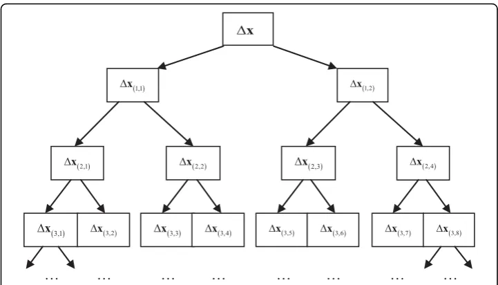
whereuandvare the projections ofΔxon the subspaces U and V, respectively. Because both the condition number and the scale of the system can be reduced after Schur complement decomposition, we propose to further decompose both the projec-tionsuand vlevel by level with the Schur complement decomposition along two paths in a tree structure, and then solve the subsystems in the Schur complement systems. Our approach is different from that proposed in [10], where only the projection vis solved in the Schur complement system. The level-by-level Schur complement decom-position can be schematically illustrated as in Figure 1. We derive the iterative system in the following discussions.
Suppose that the subsystem at the ith level is as follows
S( )i j, Δx( )i j, =b( )i j, (22)
whereS(i,j)is the Schur complement matrix with the subscript (i,j) being thejth (j= 0,
1,..., 2i) term at theith (i= 0, 1,...,L) level in the tree structure as illustrated in Figure 1. Particularly,S(0,0)is the global matrixkas defined in equation (20). To solve this system
in the Schur complement system, equation (22) will be further decomposed at thei+1th level. Thus, the solutionΔx(i,j)is firstly expressed with the bases of the two subspaces as
Δx( )i j, =( )i j, Δx(i+1 2, j−1) +( )i j, Δx(i+1 2, j) (23)
where Δx(i+1,2j-1) andΔx(i+1,2j)are the projections ofΔx(i,j)on the subspaces formed
Substituting equation (23) into equation (22) yields
S S
x
x
i j i j i j i j
i j i j , , , , , , ( ) ( ) ( ) ( ) ( + − ) + ( ) ⎡ ⎣ ⎤⎦ ⎡ ⎣ ⎢ ⎢ ⎤ ⎦ ⎥ ⎥
Δ
Δ
1 2 1 1 2
==b( )i j, (24)
Multiplying both sides of equation (24) from the left by [Γ(i,j)Ψ(i,j)]T, we can obtain
i j i j T i ji j i ji j i j
, , , , , ,
,
( ) ( ) ( ) ( ) ( ) ( ) (+ −)
⎡
⎣ ⎤⎦ ⎡⎣S S ⎤⎦
x
Δ Δ
1 2 1 x
xi j i j i j b T i j + ( ) ( ) ( ) ( ) ⎡ ⎣ ⎢ ⎢ ⎤ ⎦ ⎥ ⎥= ⎡⎣ ⎤⎦
1 2, , , ,
(25)
Thus, equation (25) can be further rewritten into a two-by-two block system
S S
S S
x
x
i j i j
i j i j
i j i , , , , , , ( ) ( ) ( ) ( ) + − ( ) + ⎡ ⎣ ⎢ ⎢ ⎤ ⎦ ⎥ ⎥ 11 12 21 22
1 2 1 1
Δ
Δ 22
1 2 j i j i j ( ) ( ) ( ) ⎡ ⎣ ⎢ ⎢ ⎤ ⎦ ⎥ ⎥= ⎡ ⎣ ⎢ ⎢ ⎤ ⎦ ⎥ ⎥ b b , , (26)
where S( )i j, 11=T( ) ( ) ( )i j, S i j, i j, , S( )i j, 12=( ) ( ) ( )Ti j, S i j, i j, , S( )i j, 21=( ) ( ) ( )Ti j, S i j, i j, , and S( )i j, 22 =( ) ( ) ( )Ti j, S i j, i j, , while the two components on the right-hand side (RHS) of equation (26) are b( )i j, 1=T( ) ( )i j, b i j, , and b( )i j, 2=( ) ( )Ti j, b i j, . From equa-tion (26), it can be seen that S(i,j)11 and S(i,j)22 correspond to the equations for the
unknowns of Δx(i+1,2j-1)and Δx(i+1,2j), respectively, while S(i,j)12and S(i,j)21define the
coupling between these two sets, which will be eliminated in the following discussions. Applying block Gaussian elimination to equation (26) leads to [22]
S S
0 S
x
x
i j i j
i j i j i j , , , , , ( ) ( ) + ( ) + − ( ) + ( ) ⎡ ⎣ ⎢ ⎢ ⎤ ⎦ ⎥ ⎥ ⎡ ⎣ 11 12 1 2
1 2 1 1 2 Δ Δ ⎢⎢ ⎢ ⎤ ⎦ ⎥ ⎥= ⎡ ⎣ ⎢ ⎢ ⎤ ⎦ ⎥ ⎥ ( ) + ( ) b b i j i j , , 1 1 2 (27) Δx
( )1,1
Δx Δx( )1,2
( )2,1
Δx Δx( )2,2 Δx( )2,3 Δx( )2,4
( )3,1
Δx Δx( )3,2 Δx( )3,3 Δx( )3,4 Δx( )3,5 Δx( )3,6 Δx( )3,7 Δx( )3,8
…
…
…
…
…
…
…
…
where S(i+1 2, j) =S( )i j, 22−S( )i j, 21S( )−i j1, 11S( )i j, 12, which is called the Schur
comple-ment with respect to S(i,j)11[7], bi j i j b S S b
T
i j i j i j i j T
i j
+
( 1 2 )= ( ) ( )− ( )21 ( )− 11 ( ) ( ) 1
, , , , , , , . From
equa-tion (27), we have
S( )i j, 11Δx(i+1 2, j−1)+S( )i j, 12Δx(i+1 2, j) =b( )i j, 1 (28)
S(i+1 2, j)Δx(i+1 2, j) =b(i+1 2, j) (29)
It can be found that the condition number of matrix S(i+1,2j)is smaller than that of
matrix S(i,j)[9]. Hence, solving the inverse problem in the Schur complement system at
thei+1th level will be more efficient than solving it at theith level. We herein solve equation (29) using the biconjugate gradient method [23]. Its advantage is that it does not square the condition number of the original equations [24]. Basically, the biconju-gate gradient method can be used to solve the large-scale systems with the fastest speed among all the generalized conjugate gradient methods in many cases [25]. The algorithm for solving equation (29) can be summarized as follows
Algorithm 1
1. Input an initial guessΔx(i+1,2j)0;
2. Initialized0=f0 =r0=p0¬ b(i+1,2j)- S(i+1,2j)Δx(i+1,2j)0;
3. Fork= 0, 1, 2... until convergence do
k
k k k k
k k k i j k
k
pkT rk
fkT i j dk
v v d
r r d
p ← +
(
)
← + ← − + + ( + ) + S S 1 2 11 1 2
,
, 1
1 1 2
1 1 1 1 1 ← − ← + + ← + ← + ( ) + + + p f p k T rk p
kT rk
d r d
f p
k k i j
T k
k
k k k k
k k
S ,
++1+k kf End for
After the derivation of Δx(i+1,2j)from equation (29) with algorithm 1, the next task is
to obtain the other component of Δx(i+1,2j-1)for the synthesis of the solution Δx(i,j).
Here,Δx(i+1,2j-1) is also solved in the Schur complement system due to its low
condi-tion number.
Eliminating the block S(i,j)12in equation (26) using block Gaussian elimination with
S(i,j)22as pivot block, we have
S 0
S S
x
x
i j
i j i j
i j i j + − ( ) ( ) ( ) + − ( ) + ( ) ⎡ ⎣ ⎢ ⎢ ⎤ ⎦ ⎥ ⎥
1 2 1
21 22
1 2 1 1 2 , , , , , Δ Δ ⎡⎡ ⎣ ⎢ ⎢ ⎤ ⎦ ⎥ ⎥= ⎡ ⎣ ⎢ ⎢ ⎤ ⎦ ⎥ ⎥ + − ( ) ( ) b b i j i j
1 2 1 2 , ,
where S(i+1 2, j−1)=S( )i j, 11−S( )i j, 12S−( )i j1, 22S( )i j, 21 and b(i+1 2, j−1)=( ) ( )Ti j, bi j, −S( )i j, 12S−( )i j1, 22( ) ( )Ti j, bi j, . Thus S(i+1,2j-1)is the Schur complement with respect toS(i,j)22.
From equation (30), we can obtain
S(i+1 2, j−1)Δx(i+1 2, j−1) =b(i+1 2, j−1) (31)
Thus, the solution Δx(i+1,2j-1) can be obtained in a same manner as in Algorithm 1,
and the only difference is that Δx(i+1,2j),S(i+1,2j), andb(i+1,2j)should be replaced with Δx(i+1,2j-1),S(i+1,2j-1), andb(i+1,2j-1), respectively. Solving equation (31) is computationally
efficient because of the reduced condition number in the Schur complement system [7]. Moreover, such a strategy of deriving both Δx(i+1,2j-1)andΔx(i+1,2j)in the Schur
complement system can be implemented in a parallel manner, since equations (29) and (31) are decoupled. Therefore the subsystem at the ith level as in equation (22) can be decomposed into the two linear subsystems at the i+1th level, i.e., Schur com-plement systems as in equations (29) and (31). After obtaining Δx(i+1,2j-1)andΔx(i+1,2j),
they are then substituted into equation (23) to yield the solution Δx(i,j)at theith level.
The whole reconstruction algorithm is summarized as follows
Algorithm 2
1. Setx0 to an initial guess;
2.x¬ x0, calculatebandkat xin equation (20) with the adaptive regularization
scheme as in equation (19);
3. The global system of equation (20) is decomposed with the Schur complement system level by level in a same manner as the decomposition of equation (22) into equations (29) and (31) to obtain the subsystemS(i,j)Δx(i,j)=b(i,j)at theith level for i=1,...,Land j=1,..., 2i, the subspaces at theith level are formed by the columns of
Γ(i,j)andΨ(i,j), respectively;
4. Seti=L;
Forj= 1,..., 2ido
Combining equations (26), (27), and (30), solveS(i+1,2j)Δx(i+1,2j)=b(i+1,2j)and
S(i+1,2j-1)Δx(i+1,2j-1) =b(i+1,2j-1) with Algorithm 1, where Δx(i+1,2j-1), S(i+1,2j-1), and
b(i+1,2j-1) are used instead of Δx(i+1,2j), S(i+1,2j), and b(i+1,2j) when Algorithm 1 is
employed for the latter case; End for
5. Whilei≥0
{
Forj= 1,..., 2ido
Substitute the solutionsΔx(i+1,2j)andΔx(i+1,2j-1)into equation (23) to obtain the
solution Δx(i,j)at theith level;
End for
i=i- 1; }
7. If ||Δx(0,1)|| >ε
go to 2; Else
x ¬x0, outputx.
As mentioned before, the Schur complement system has a smaller condition number than that of the system from which it is constructed [7]. As a result, iterative methods based on the Schur complement systems can be more efficient than the methods based on the global matrix as in equation (20) due to its reduced scale and the smaller condition number. Therefore, the proposed algorithm can be expected to be more effi-cient than the conventional ones, as the results demonstrated in the next section.
Results and Discussion
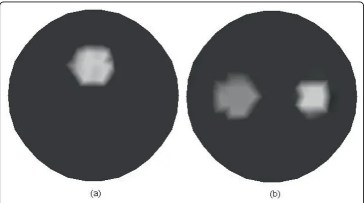
In this work, assuming that the scattering coefficients are known, we focus on the recon-struction of the absorption coefficientμaxf. Two phantoms as illustrated in Figure 2 are used
to evaluate the proposed algorithm. Figure 2(a) contains one object, and Figure 2(b) contains two objects of different shapes. Table 1 and Table 2 outline the optical and fluorescent para-meters in different regions of the simulated phantoms corresponding to Figures 2(a) and 2(b), respectively. Four sources and thirty detectors are equally distributed around the cir-cumference of the simulated phantom. The simulated forward data are obtained from equa-tions (1) and (2), in which Gaussian noise with a signal-to-noise ratio of 10dB is added to evaluate the noise robustness of the algorithms. The parametersc1andc2in equation (19) are, respectively, set to 0.2 and 2. The initial guesses for solutionsΔx(i+1,2j)andΔx(i+1,2j-1)of
equations (29) and (31) are set to 0. The initial value ofx0is set to 5mm-1. The subspace
created from the right singular vectors of the singular value decomposition (SVD) is optimal. Since SVD is computationally expensive, it is expected that a subspace close to SVD sub-space will do almost as good. Thus, the choice of an oscillatory basis can be a basis created
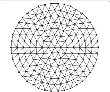
by sine or cosine functions with increasing frequency [26]. Here discrete cosine basis is employed in the simulations. To reliably evaluate the performance of different methods for the inverse problem, the best way is to use an independent forward model, which is different from the one employed in the inverse problem, to generate the synthetic data [27]. There-fore, in our case, a finer mesh as shown in Figure 3 with 169 nodes and 294 triangular ele-ments is used to generate the forward simulated data.
Table 1 Optical and fluorescent properties of one-object phantom
Excitation light μaxf(mm-1) μaxi(mm-1) ′sx(mm−1) q τ(ns)
Background 0.06 0.02 5.0 0.3 0.5
Object 0.2 0.02 5.0 0.3 0.5
Emission light μamf(mm-1) μami(mm-1) ′ −
sm(mm )
1 q τ(ns)
Background 0.006 0.01 2.0 0.3 0.5
Object 0.1 0.01 2.0 0.3 0.5
Table 2 Optical and fluorescent properties of two-object phantom
Excitation light μaxf(mm-1) μaxi(mm-1) ′ −
sx(mm1) q τ(ns)
Background 0.06 0.02 5.0 0.3 0.5
Objects 0.15, 0.2 0.02 5.0 0.3 0.5
Emission light μamf(mm-1) μami(mm-1) ′ −
sm(mm 1) q τ(ns)
Background 0.002 0.01 2.0 0.3 0.5
Objects 0.03, 0.05 0.01 2.0 0.3 0.5
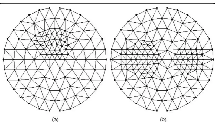
It is well known that the most significant superiority of the anatomical imaging mod-ality lies in the high spatial resolution. Hence, it will be helpful to improve the image quality and accelerate the reconstruction process if we use the anatomical image as prior information for mesh generation. The reconstructed domain is firstly uniformly discretized according to the Delaunay triangulation scheme, after which the uniform mesh is refined only for the areas with large variations of the pixel values. To simulate this idea, we employ the images shown in Figures 4(a) and 4(b) with a resolution of 100 × 100 pixels as the prior images corresponding to Figures 2(a) and 2(b), respec-tively. The meshes are generated as shown in Figure 5 for the inverse problem of FMT. The mesh with 122 nodes and 212 triangular elements (Figure 5(a)), and the
Figure 4Model of prior image. (a) The prior image corresponds to Figure 2(a), and (b) the prior image corresponds to Figure 2(b).
mesh with 148 nodes and 264 triangular elements (Figure 5(b)) are generated incorpor-ating the prior information as shown in Figures 4(a) and 4(b), respectively.
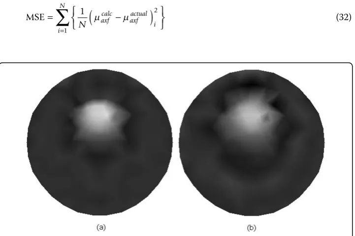
Figures 6(a) and 6(b) show, respectively, the reconstructed images of μaxffor one
object phantom using the adaptive regularization scheme and Tikhonov regularization method. Figures 7(a) and 7(b) depict the results for two objects phantom from the above two different algorithms. Here, both of the results from Figures 6 and 7 are based on the CG method. As seen from Figures 6 and 7, better reconstructed results can be achieved from the adaptive regularization scheme. To quantitatively assess the accuracy of the different algorithms, the mean square error (MSE) is introduced
MSE = ⎧⎨
(
−)
⎩
⎫ ⎬ ⎭ =
∑
1 21 N
axfcalc axfactual i i
N
(32)
Figure 6Reconstructed images of absorption coefficient due to exogenous fluorophoresμaxffor one object. (a) Reconstructed result with the adaptive regularization scheme, and (b) reconstructed result with the Tikhonov regularization method.
whereNis the total number of nodes in the domain. The superscriptcalc denotes the values obtained using reconstruction algorithms; and actualdenotes the actual dis-tribution of μaxf which is used to generate the synthetic image data set. Table 3 lists
the performance of the reconstruction algorithms in terms of MSE. It can be seen that the adaptive regularization scheme can significantly improve the quality of the recon-structed images and achieve a smaller MSE in either case.
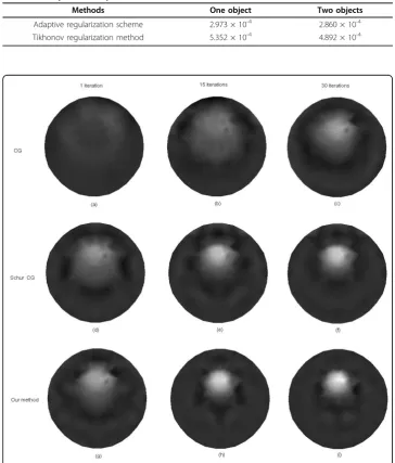
Figure 8 shows the reconstructed images of μaxffor one object phantom using the
different algorithms after 1, 15, and 30 iterations, respectively. After 30 iterations, the reconstructed image from the proposed algorithm has a relatively higher contrast than those obtained from the other two algorithms. Figure 9 depicts the reconstructed
Table 3 Comparison of performance of methods
Methods One object Two objects
Adaptive regularization scheme 2.973 × 10⁻⁴ 2.860 × 10⁻⁴
Tikhonov regularization method 5.352 × 10⁻⁴ 4.892 × 10⁻⁴
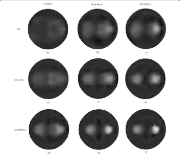
images of μaxf for two objects phantom using the different algorithms, from which it
can be seen that the proposed method can reconstruct the images more accurately than the other two methods even after the first iteration. According to the third col-umn of Figure 9, the reconstructed image quality based on our algorithm is signifi-cantly improved as compared with that based on the other two methods.
We investigated how the MSE changed against the number of iterations for different algorithms. Figure 10 shows a fast convergence of our algorithm with a less MSE than the other two algorithms. In addition, the CG method converges slower than the Schur CG method and our method, which means that solving the inverse problem based on the Schur complement system is superior to that based on the global system. The computation time of different algorithms is further investigated in our work to evaluate the convergence rate. Table 4 lists the computation time after 30 iterations for different algorithms. From this table, it can be seen that the time needed for our algorithm after 30 iterations is less than that of the Schur CG method. Although the former is a little bit longer than the time needed for the CG method, our algorithm needs only less than 5 iterations to achieve the precision of the CG method after 30 iterations. As a result, the CG method needs much more iterations to achieve a given precision of reconstruction than our method. Therefore, compared with the other two methods, the proposed algorithm is more efficient and stable.
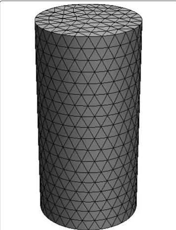
To further validate the proposed algorithm for 3D reconstruction, a phantom as illu-strated in Figure 11 is used for simulations. Within this phantom, a small cylindrical object is suspended. In Figure 11, the dashed curves represent the planes of measure-ments. Four sources and sixteen measurements are used for each plane in the simula-tions. The mesh for reconstructing the 3D image is shown in Figure 12, which contains 858 nodes and 3208 tetrahedral elements. Figures 13 and 14 depict the recon-structed 2D cross sections of the 3D phantom shown in Figure 11 using the Schur CG method and the proposed algorithm, respectively. Table 5 lists the performance of the
40mm
20mm
Figure 11Simulated phantom for 3D reconstruction. The phantom of radius 10mm and height 40mmwith a uniform background ofμaxf= 0.005mm-1, which is positioned atx= 10mm,y= 0mmand
z= 20mm. The small cylindrical anomaly has a radius of 2mmand height 6mmwithμaxf= 0.01mm-1. The anomaly is positioned atx= 15mm,y= 0mmandz= 20mm. The dashed curves represent the measurement planes, atz= 15mm,z= 20mm,z= 25mm.
Table 4 Computation time of FMT image reconstruction for 30 Iterations
Methods One object Two objects
CG 62s 86s
Schur CG 203s 281s
Our algorithm 141s 179s
above two methods for a quantitative comparison. From this table, we can conclude that our proposed algorithm can also speed up the reconstruction process and achieve high accuracy for the 3D case.
Conclusion
parameter is determined adaptively according to the objective function. Simulation results demonstrate that the proposed method outperforms the previous methods, such as the CG and the Schur CG methods, in both reconstruction accuracy and speed.
Acknowledgements
This research is supported by the National Natural Science Foundation of China, No.60871086, the Natural Science Foundation of Jiangsu Province China No.BK2008159, the CSC Scholarship, PolyU, and ARC grants.
Author details
1School of Electronics and Information Engineering, Soochow University, Suzhou 215021, China.2Department of
Electronic and Information Engineering, Hong Kong Polytechnic University, Hong Kong.3School of Information Technologies, University of Sydney, Sydney, NSW 2006, Australia.4Med-X Research Institute, Shanghai Jiao Tong University, Shanghai 200030, China.
Authors’contributions
WZ conceived the study, implemented the algorithm, and drafted the initial manuscript. JJW participated in the design of the study, analyzed the simulation results, and helped to draft the manuscript. DDF critically reviewed the manuscript, helped to analyze the results, revised the manuscript, and provided the valuable advice.
Competing interests
The authors declare that they have no competing interests.
Received: 31 December 2009 Accepted: 20 May 2010 Published: 20 May 2010
Figure 14Reconstructed images using the proposed algorithm. Reconstructed images using the proposed algorithm, which are 2D cross sections through the reconstructed 3D volume. The right-hand side corresponds to the top of the cylinder (z= 40mm), and the left corresponds to the bottom of the cylinder (z= 0mm), with each slice representing a 10mmincrement.
Table 5 Performance comparison of reconstruction methods for 3D case
Methods Schur CG Our algorithm
Computation time (s) 3527 2215
MSE 3.629 × 10⁻³ 1.241 × 10⁻³
References
1. Boas DA, Brooks DH, Miller EL, DiMarzio CA, Kilmer M, Gaudette RJ, Zhang Q:Imaging the body with diffuse optical tomography.IEEE Signal Processing Mag2001,18:57-75.
2. Ntziachristos V:Fluorescence Molecular Imaging.Annual Review of Biomedical Engineering2006,8:1-33. 3. Ntziachristos V, Ripoll J, Wang LHV, Weissleder R:Looking and listening to light: the evolution of whole-body
photonic imaging.Nat Biotechnol2005,23:313-320.
4. Milstein AB, Oh S, Webb KJ, Bouman CA:Direct reconstruction of kinetic parameter images in fluorescence optical diffusion tomography.IEEE International Symposium on Biomedical Imaging2004, 1107-1110.
5. Reynolds JS, Troy TL, Mayer RH, Thompson AB, Waters DJ, Cornell KK, Snyder PW, Sevick-Muraca EM:Imaging of spontaneous canine mammary tumors using fluorescent contrast agents.Photochem Photobiol1999,70:87-94. 6. Fedele F, Eppstein MJ, Laible JP, Godavarty A, Sevick-Muraca EM:Fluorescence photon migration by the boundary
element method.J Comput Phys2005,210:109-132.
7. Axelsson O:Iterative Solution MethodsCambridge University Press 1994.
8. Tarvainen T, Vauhkonen M, Arridge SR:Gauss Newton reconstruction method for optical tomography using the finite element solution of the radiative transfer equation.J Quant Spectrosc Radiat Transfer2008,109:2767-2778. 9. Haynsworth E:On the Schur complement.Basel Math Notes1968,20.
10. Zhao B, Wang H, Chen X, Shi X, Yang W:Linearized solution to electrical impedance tomography based on the Schur conjugate gradient method.Meas Sci Technol2007,18:3373-3383.
11. Silva AD, Dinten JM, Peltié P, Coll JL, Rizo P:In vivo fluorescence molecular optical imaging: from small animal towards clinical applications.16th Mediterranean Conference on Control and Automation, Congress Centre, Ajaccio, France2008, 1335-1340.
12. Gibson AP, Hebden JC, Arridge SR:Recent advances in diffuse optical imaging.Phys Med Biol2005,50:R1-R43. 13. Lin Q:Basic text book of numerical solution method for differential equationScience Press, 22003.
14. Paithankar DY, Chen AU, Pogue BW, Patterson MS, Sevick-Muraca EM:Imaging of fluorescent yield and lifetime from multiply scattered light reemitted from random media.Appl Opt1997,36:2260-2272.
15. Arridge SR, Schweiger M:A general framework for iterative reconstruction algorithms in optical tomography using a finite element method.Computational Radiology and Imaging: Therapy and DiagnosisIMA Volumes in Mathematics and Its Applications, Springer-VerlagBorgers C, Natterer F 1998,110:45-70.
16. Magnus JR, Neudecker H:Matrix Differential Calculus with Applications in Statistics and Econometrics.Wiley Series in Probability and StatisticsNew York: Wiley 1988.
17. Kaipio J, Somersalo E:Statistical and Computational Inverse ProblemsSpringer 2005.
18. Roy R, Godavarty A, Sevick-Muraca EM:Fluorescence-Enhanced Optical Tomography Using Referenced Measurements of Heterogeneous Media.IEEE Trans Med Imaging2003,22:824-836.
19. Tikhonov AN, Arsenin VY:Solution of Ill-Posed ProblemsWashington, DC: Winston 1977.
20. Pogue BW, Patterson MS, Farrell TJ:Forward and inverse calculations for 3-D frequency-domain diffuse optical tomography.In Optical Tomography, Photon Migration, and Spectroscopy of Tissue and Model Media: Theory, Human Studies, and Instrumentation. Proc SPIE 2389Chance B, Alfano RR 1995, 328-339.
21. Pogue BW, McBride TO, Prewitt J, Osterberg UL, Paulsen KD:Spatially variant regularization improves diffuse optical tomography.Appl Opt1999,38:2950-2961.
22. Jennings A:Matrix ComputationWiley 1992.
23. Sarkar TK:On the Application of the Generalized BiConjugate Gradient Method.J Electromagnetic Waves and Applications1987,1:223-242.
24. Liu SW, Sung JC, Lin MS:Scattering of antiplane impact waves by cracks in a layered elastic solid.Computer Methods in Applied Mechanics and Engineering1998,156:335-349.
25. Langtangen HP, Tveito A:A numerical comparison of conjugate gradient-like methods.Comm Appl Numer Methods
1988,4:793-798.
26. Jacobsen M:Two-grid iterative methods for ill-posed problems.Master ThesisTechnical University of Denmark, Denmark 2000.
27. Colton D, Kress R:Inverse Acoustic and Electromagnetic Scattering TheorySpringer 1998.
doi:10.1186/1475-925X-9-20
Cite this article as:Zouet al.:Image reconstruction of fluorescent molecular tomography based on the tree structured Schur complement decomposition.BioMedical Engineering OnLine20109:20.
Submit your next manuscript to BioMed Central and take full advantage of:
• Convenient online submission
• Thorough peer review
• No space constraints or color figure charges
• Immediate publication on acceptance
• Inclusion in PubMed, CAS, Scopus and Google Scholar
• Research which is freely available for redistribution Submit your manuscript at