Prime Numbers and Polynomials

UNIVERSIT `

A DEGLI STUDI DI TRENTO

Facolt`

a di Scienze Matematiche, Fisiche e Naturali

DOTTORATO DI RICERCA IN MATEMATICA XXIII CICLO

A thesis submitted for obtaining the degree of Doctor of Philosophy

Luca Goldoni

PhD Thesis

PRIME NUMBERS

AND

POLYNOMIALS

Advisor:

Prof. Alberto Perelli

c

Copyright by Luca Goldoni

Abstract

Acknowledgments

“All men dream: but not equally.

Those who dream by night in the dusty recesses of their minds wake in the day to find that it was vanity:

but the dreamers of the day are dangerous men,

for they may act their dream with open eyes to make it possible. This I did.”

T.E. Lawrence (Lawrence of Arabia) Seven Pillars of Wisdom

To my wife

Gloria Isabella Mandagie and my daughter

Lucia Goldoni as well as

Contents

I

Some background

11

1 Polynomials in one variable 13

1.1 Introduction . . . 13

1.2 Primes in arithmetic progressions . . . 14

1.2.1 Sketch Proof of Dirichlet’s Theorem . . . 14

1.3 Conjectures . . . 17

1.3.1 The conjecture of Bouniakowsky . . . 17

1.3.2 The conjecture of Dickson . . . 18

1.3.3 The conjecture of Schinzel and Sierpinski . . . 18

1.3.4 The conjecture of Bateman and Horn . . . 18

1.3.5 The Hardy-Littlewood Circle Method . . . 20

1.3.6 The conjectures of Hardy and Littlewood . . . 25

2 Polynomials in several variables 27 2.1 Quadratic polynomials . . . 27

2.2 Higher degree polynomials . . . 28

2.3 Primes in non-polynomial sequences with low density . . . 31

II

The results of Pleasants

33

3.2 Preliminaries . . . 36

3.3 Notation . . . 37

3.4 The First Theorem of Pleasants . . . 38

3.5 The heuristic . . . 38

3.6 The setup for the proof: the bilinear forms . . . 39

3.7 The cubic exponential sum: the use ofS∗_{(α,B) . . . 46}

3.8 The estimation of S∗_{(α,B, P) ifh(C) =n . . . 54}

3.10 The estimates of S(α) and Sa,q . . . 65

3.11 Minor arcs . . . 68

3.12 Major arcs . . . 72

3.13 The singular series . . . 78

3.14 The proof of the first theorem of Pleasants . . . 79

4 The second theorem of Pleasants 87 4.1 Introduction . . . 87

4.2 Preliminaries . . . 88

4.3 Notation . . . 89

4.4 The Auxiliary Theorem . . . 89

4.5 The Second Theorem of Pleasants . . . 91

4.6 Theorems about Quadratic polynomials . . . 92

4.6.1 Elementary Lemmas . . . 92

4.6.2 Exponential sums . . . 94

4.6.3 Minor arcs . . . 101

4.6.4 The Major arcs . . . 103

4.6.5 The singular series . . . 106

4.7 The proof of the Auxiliary Theorem . . . 107

4.8 A Corollary of the Auxiliary Theorem . . . 109

4.9 Further Lemmas . . . 111

4.10 Cubic polynomials . . . 127

4.10.1 Introduction . . . 127

4.11 The proof of the second theorem of Pleasants . . . 131

4.11.1 Introduction . . . 131

4.11.2 The proof in Case A . . . 132

4.11.3 The proof in Case B . . . 141

III

Some results

149

5.2 Results about the h invariant . . . 153

5.2.1 Introduction . . . 153

5.2.2 Example . . . 154

5.2.3 Further examples . . . 156

6 Algorithms 167

6.1 How to find the primes of the form x2_+y4 _{. . . 167}

6.1.1 Introduction . . . 167

6.1.2 The algorithm . . . 168

6.2 How to find the primes of the form x3_{+ 2y}3 _{. . . 172}

6.3 How to find the primes of the forms x2_{+ 1 . . . 174}

IV

Appendices

177

B.2 Brun’s Sieve . . . 183

B.3 The Selberg Sieve . . . 183

B.4 The Large Sieve . . . 184

B.5 The parity problem . . . 184

C Some graphics 187 D Notation 191 D.1 Sets . . . 191

D.2 Algebra . . . 192

D.3 General Functions . . . 192

D.4 Arithmetical Functions . . . 192

D.5 Miscellaneous . . . 193

E Some useful results 195 F Elementary algebra of cubic forms and polynomials 201 F.1 Cubic forms . . . 201

F.2 Cubic polynomials . . . 203

G The polynomial of Matiyasevich 205 G.1 Introduction . . . 205

Part I

Chapter 1

Polynomials in one variable

1.1

Introduction

Since form the time of Euclid it is known that there exists an infinite set of prime numbers. The proof by Euclid [11] is the following: assume there are only finitely many primes, say p1...pm and consider the number

Q=

m

Y

k=1

pk+ 1.

Either Q is prime or there exists a prime q such that q_|Q. If Q is prime we have a contradiction because Q > pk for every k = 1...m. If Q is not

a prime it follows that q ₆= pk for k = 1...m because none of the primes

amongpk dividesQ. So even in this case we have a contradiction. If we read

the result in a different way, we can say that among the polynomials in one variable, there exists one which assumes infinitely many prime values, namely

P(x) = x. It is natural ask if this result can be generalized in some way. Actually in some special cases, if one try to imitate Euclid’s method, it is possible to prove that polynomials of the form P(x)=mx+qwitha, b_∈Nand (a, b) = 1 contains infinitely many primes among their values. For instance Euclid’s method is working with the polynomial P(x) = 4x+ 3. Many other special cases are tractable with elementary arithmetic methods,1 _{but so far}

no purely arithmetic proof is known in the general case.

1_{See [27] for a characterization of arithmetic progressions which are tractable with some}

1.2

Primes in arithmetic progressions

The first correct proof for the general case of an arithmetical progression, goes back to Dirichlet [10] after a faulty proof by Legendre [20]. Dirichlet proved that

P(x) = qx+a.

the condition (a, q) = 1 is necessary and sufficient in order to takes infinitely many prime values. Dirichlet’s original proof of this theorem is analytic and non-elementary: this means that tools from Complex Analysis has been used. An “elementary” proof was found, much later, by Selberg [37]. The word “elementary”, in this case, is a short-cut for the statement“without the use of Complex Analysis” and it does not mean, in any way, “simple”. Actually it is rather complicated. The Dirichlet’s proof is a very deep and broad generalization of an Euler’s idea. I shall try to get a very basically sketch of it.

1.2.1

Sketch Proof of Dirichlet’s Theorem

ζ(s) = ∞

X

n=1

1

ns s∈ R, s >1. (1.1)

and he showed that it has a deep and profound connection with prime numbers. Namely, due tounique factorizationin the ring of integers the following formula hold:

ζ(s) =Y

p_∈P

1₋ 1

ps

−1

s_∈R, s >1.

• Euler considered

lim

s_→1+ζ(s).

and due to the divergence of harmonic series, he was able to show that

lim

s→1+log

Y

p∈P

1− 1 ps

−1

=∞.

Upon taking logarithms of both sides in (1.1) and discarding negligible terms, this implies that

X

p∈P 1

This of course implies that the set of primes in infinite and, for the first time provides an analytic method to deal with similar problems. That’s why it mark’s the beginning of Analytic Number Theory.

• Dirichlet generalized Euler’s method but he had to set some non triv-ial modifications to it. The main reason for this is that, while the characteristic function of the progression P(x) = 2x+ 1 is totally mul-tiplicative and leads to the “Euler product” as in the ζ function, the the characteristic functions of any other arithmetic progression has no longer this property.

• In order to overcome this problem, Dirichlet introduced a special kind of functions now called “Dirichlet characters”which may regarded as a sort of “arithmetical harmonics” in the sense that they play the role of what we now call “an orthogonal basis in a finite Fourier Analysis context. I shall quote definition and the most important properties of the characters.

– A completely multiplicative arithmetic periodic function χ:Z_→C.

with period m that is not identically zero is called a Dirichlet character with conductor q.

– For everymthere are exactlyϕ(q) Dirichlet characters whereϕ(q) stands for the Euler’s totient function.

– The character

χ0(n) =

1 if (n, m) = 1 0 otherwise.

is called “principal character”

– The Dirichlet characters with conductorqform amultiplicative groupwith φ(q) elements and identity element χ0

– For every character χ and every character χ′ _{we have} 1

φ(q)

X

n( mod q)

χ(n)χ′_{(n) =}

1 if χ=χ′

0 otherwise. (1.2)

• For every character χ and for every integers n, a,we have 1

φ(q)

X

χ( modq)

χ(n)χ(a) =

1 if n≡a (modq)

• The relations (1.2) and (1.3) are called“Orthogonality Relations”

and in some sense they let us remember the well known orthogonality relations inClassical Fourier Analysis.

• For each character Dirichlet defined the function

L(s, χ) = ∞

X

n=1 χ(n)

ns s∈R s >1.

The series on the right hand side is a special cases of more general series called Dirichlet series.

• For each L-series we have

L(s, χ) =Y

p

1₋ χ(p)

ps

−1

s >1.

because χis totally multiplicative.

• Moreover we have

logL(s, χ) =X

p_∈P

∞

X

k=1 χ(pk₎

kpsk .

• Using the orthogonality relations we have 1

φ(q)

X

χ

χ(a) logL(s, χ) =X

p∈P ∞

X

k=1

X

pk_{≡a( modq)}

1

kpsk .

and from this, after some calculations 1

φ(q)

X

χ

χ(a) logL(s, χ) = X

p_≡a( mod q)

1

ps +O(1). (1.4)

ass_→1+_.

• It is quite easy to show that

L(s, χ0) =ζ(s)Y

p|m

1₋ 1

ps

.

and so that

lim

• If one is able to show that χ ₆= χ0 imply L(1, χ)6= 0 for all χ of

con-ductor m, then immediately it follows that there are infinitely many primes pof the form p≡a( mod q). So this is the crux of Dirichlet’s proof. The difficult part of Dirichlet’s proof is showing L(1, χ)₆= 0 for

real characters i.e for characters which take only real values. Any-way Dirichlet was able to do this and produced a valid proof. At the present, for polynomials inone variable, this is the only case where it is possible to reach a result of this kind. Not only it is not known any example of a polynomial in one variable with degree d > 1 producing infinitely many primes but even worse, it is not known if a such poly-nomial does exists. In other words, even no result of “pure existence

” (possibly non-constructive) is known. Roughly speaking, in handling such a kind of polynomials, the difficulties arise from the fact that the values of them are “widely scattered” among the integers. For this kind of polynomials there are, at the present, only conjectures as illustrated in the following section.

1.3

Conjectures

1.3.1

The conjecture of Bouniakowsky

Let P(x) _∈ Z[x]: in order to represent infinitely many primes, trivially, it must be irreducible. However this conditions is by no means enough to ensure that the range of the polynomial contains an infinite subset of primes. In order to show why it is so, one can consider the following simple example:

Example 1.1. Let P(x) =x2_{+x+ 2. This is an irreducible polynomial in}

Z[x] but his values are all even because if we write P(x) =x(x+ 1) + 2.

we notice that the right hand side is the sum of two even numbers.

In 1857 Bouniakowsky [2] made a conjecture concerning prime values of polynomials that would, for instance, imply that P(x) = x2 _{+ 1 is prime}

for infinitely many integers x.

Conjecture 1.1. Let P(x)be a polynomial in Z[x] and define the fixed divi-sor of P(x) , written d(P), as the largest integer d such that d divides P(x)

1.3.2

The conjecture of Dickson

In [9] Dickson stated the following conjecture

Conjecture 1.2. Let

L=_{Pj(x) =qjx+aj ∈Z[x] , ∀ j = 1· · ·k}.

any finite set of linear polynomials with qj ≥ 1 and (qj, aj) = 1 for every

j = 1...k. Suppose that no integerm >1 divides P(x)P2(x)...Pk(x) for every

x _∈ N. Then there are infinitely many natural numbers n for which all the numbersP1(n)...Pk(n) are simultaneously primes.

1.3.3

The conjecture of Schinzel and Sierpinski

In [35] Schinzel stated the following conjecture better known as “Schinzel’s hypothesis H” which is a wide generalisation of a Dickson’s conjecture.

Conjecture 1.3. Let

P={Pj(x)∈Z[x] , j = 1· · ·k}.

any finite set of irreducible polynomials in one variable with positive leading coefficients . Suppose that no integer m > 1 divides P(x)P2(x)...Pk(x) for

every x∈N. Then there are infinitely many natural numbers n for which all the numbers P1(n)...Pk(n) are simultaneously primes.

1.3.4

The conjecture of Bateman and Horn

In [1] Bateman and Horn made the following

Conjecture 1.4. Let

P=_{Pj(x)∈Z[x] , j = 1· · ·k}.

any finite set of polynomials in one variable with positive leading coefficients, and of degreeh1...hk respectively. Let each of these polynomials is irreducible

over the field of rational numbers and no two of them differ by a constant factor. Let

A =_{n _∈N: 1_≤n_≤N, Pj(n)∈P ∀j = 1· · ·k}.

Finally, let

then

Q∼(h1· · ·hk)−1C(P1,· · ·Pk) N

Z

2

1

logk(t)dt. (1.5)

where

C(P1,· · ·Pk) =

Y

p_∈P

1₋1

p

−1

1₋ w(p)

p

.

being w(p) the number of solutionsx of the congruence P1(x)P2(x)_{· · ·}Pk(x)≡0 mod p.

with 1_≤x_≤p.

The heuristic argument in support of (1.5)essentially amounts to the fol-lowing. From the PNT, in some sense, the chance that a large positive integer

m is prime is around _log1_m. Since

Pj(n) =a0jnhj+a1jnhj−1+. . . ahjj =a0jn

hj

1 + a1j

a0jn

+· · · ahjj

a0jnhj

.

we have that and so logPj(n) ≈ hjlogn. If we could treat the values of

these polynomials at n as independent random variables, then the chance that they would be simultaneously prime at n would be

k

Y

j=1

1 logPj(n)

=

k

Y

j=1

1

hjlogn

= (h1· · ·hk)−1log−k(n).

and hence we would expect

Q_≈(h1_{· · ·}hk)−1 N

X

n=2

log−k(n). (1.6)

However, the polynomials P1...Pk are unlikely to behave both randomly and

independently. For example, if P1(x) = x and P2(x) = x+ 2 we have that eitherP1(n), P2(n) are both even or they are both odd. Thus for each prime p we must apply a correction factorkp =rp/sp where

• rp is the chance that for random n none of the integers P1(n), ...Pk(n)

is divisible by p.

• spis the chance that none of the integers in a random k-tuple is divisible

If we remember the meaning ofw(p),we have that

rp =

p−w(p)

p = 1− w(p)

p .

Moreover

sp =

1₋ 1

p

k

.

because the chance of xj being divisible by p is 1/p and we have that the

element of the k-tuple are independent. So the correction factor for (1.6) is

C(P1,· · ·Pk) =

Y

p

kp =

Y

p∈P

1₋ 1

p

−1

1₋ w(p)

p

.

which leads to

Q_∼(h1_{· · ·}hk)−1C(P1,· · ·Pk) N

X

n=2

1 logk(t).

which is essentially the same as the approximation given in (1.5). The con-jecture of Bateman-Horn is stronger than the concon-jecture of Bouniakowsky and is a quantitative version of the conjectures of Schinzel and Sierpinski. The truth of this conjecture is known only in the case n = 1. In this case the conjecture is equivalent to the Dirichlet’s theorem.

1.3.5

The Hardy-Littlewood Circle Method

I shall get an informal introduction to the Hardy-Littlewood Circle Method. At this stage the main purpose of this introduction is to explain the tool by means of which Hardy and Littlewood were able to formulate some conjec-tures about polynomials. The Circle Method is a clever idea for investigating many problems in additive number theory. It originated in investigations by Hardy and Ramanujan [14] on the partition function p(n). Now it is a foundamental tool in Analytic Number Theory and in particular in Additive Number Theory. Consider the problem of writing n as a sum of s perfect

k-powers. Ifk = 1 there is a quite simple combinatorial solution: the number of ways of writing n as a sum of s non-negative integers is

r1,s(n) =

n+s₋1

s−1

Unfortunately, the combinatorial argument does not generalize to higher k. There is another method, of analytical type which solves the k= 1 case and can be generalized. Let z ∈C with |z|<1, then the series

f(z) = ∞

X

m=0 zm_.

is convergent and we have

f(z) = 1 1−z.

From now on, we shall call this function as “generating function”. Let

r1,s(n) denote the number of solutions to the equation

m1+_{· · ·}ms =n.

where each mi is a non-negative integer. We claim that

(f(z))s= ∞

X

m1=0

zm1

!

· · ·

∞

X

ms=0

zms

!

= ∞

X

n=0

r1,s(n)zn. (1.7)

This follows by expanding the product in (1.7) and collecting the products

zm1_{· · ·z}ms _=zm1+···ms_.

of the same degree n=m1+...ms. On the other hand, we have

(f(z))s=

1 1₋z

s

= 1

(s₋1)!

ds₋1 dzs₋1

1 1₋z

.

and so

(f(z))s= 1 (s₋1)!

ds₋1 dzs₋1

∞ X n=0 zn ! = ∞ X n=0

n+s₋1

s−1

zn_.

which yields

r1,s(n) =

n+s−1

s−1

.

Actually, it is easy to see that all series does converge so this kind of approach is not only formal but analytical and, more important, this method of proof can be generalized. I shall try to get a very basically sketch of it. LetAsome given subset of Nand s a positive integer. We define the formal series

FA(z) =

X

a_∈A

and we call it, as before, “generating function”. Next, we write

(FA(z))s =

X

a∈A

za

!s

= ∞

X

n=1

r(n, s, A)zn.

It is not hard to prove thatr(n;s, A) is the number of ways of writing n as a sum of s elements of A. In order to extract individual coefficients from a power series we have the following standard fact from Complex Analysis. As it is well known if γ stand for the unit circle of center O in the complex plane, oriented counter-clockwise then

1 2πi

Z

γ

zndz =

1 if n=−1 0 otherwise.

so, if we have a power series with radius of convergence larger than one,

G(z) = ∞

X

k=0 akzk.

then

1 2πi

Z

γ

G(z)z−(n+1)_{dz =a}

n.

Consequently, if for a while we ignore convergence problems this result yields

r(n, s, A) = 1 2πi

Z

γ

(FA(z))sz−(n+1)dz.

An alternative, but equivalent, formulation is to consider a different gener-ating function forA. If we set

e(α) = e2πiα.

the immediately we see that

1

Z

0

e(nα)e(₋mα)dα=

1 if n=m

0 otherwise.

Now we have that the generating function is

fA(α) =

X

a_∈A

and

1

Z

0

(fA(α))se(−nα)dα =r(n, s, A).

again, ignoring for now any convergence problems. If we can evaluate the above integral, not only will we know which ncan be written as the sum ofs

elements ofA, but we will know in how many ways. This is the basic formal context for the circle method. Now we turn to convergence issues. If A is an infinite subset 2 _{the defining series for the generating function f}

A(x) need

not converge, or may not have a large enough radius of convergence. We get around this trouble in the following way: for each N, we define

AN ={a∈A:a≤N}.

For each N, we consider the truncated generating function attached to AN:

fN(α) =

X

a∈AN

e(aα).

As fN(α) is a finite sum, all the convergence issues vanish. A similar

argu-ment as before yields

(fA(α)) s

= X

n_≤sN

rN(n, s, A)e(nα).

where, in this case,rN(n, s, A) is the number of ways of writingn as the sum

of s elements ofA with each element at most N. But ifn ≤N then

rN(n, s, A) =r(n, s, A).

because no element ofAgreater thannis used in representing n. So we have proved

Proposition 1.1. If n _≤N then

r(n, s, A) = rN(n, s, A) =

1

Z

0

(fN(α)) s

e(₋nα)dα. (1.8)

However, having an integral expression for rN(n, s, A) is not enough: we

must be able to evaluate the integral either exactly, or at least bound it away from zero. We notice that fN(α) is defined as a sum of AN terms, each of

2_{IfAis finitewe can just enumeratea}

absolute value 1 but if this terms does have a “random” distribution on the unit circle, the size of_|fN(α)|should be much smaller than the trivial upper

bound N. This is the so called “Philosophy of Square-root Cancella-tion”: in general, if one adds a “random” set ofN numbers of absolute value 1, the sum could be as large as N, but often is roughly at most of size √N.

3 _{In many problems, for mostα∈[0,1] the size off}

N(α) is about

√

N while for special α _∈ [0,1], the size of fN(α) is about |N|. We expect the main

contribution to come fromα _∈[0,1] where fN(α) is large so

1. If the contribution of the set of these α can be evalutated. 2. If we can show that the contribution of the remaining α is

smaller.

then we will have that rN(n, s, A) is bounded away from zero. In order to

do this we split [0,1] into two disjoint subsets: the so called theMajor arcs Mand Minor arcs m. So

r(n, s, A) =

Z

M

(fN(α))se(−nα)dα+

Z

m

(fN(α))se(−nα)dα.

The construction of M and m depend on N and the problem under inves-tigation. On the Major arcs _M we must be able to find a function which, up to lower order terms, agrees with (fN(α))s and is easily integrated. This

will be the contribution over the Major arcs and must be of a “good shape” away from zero and possibly tends to infinity with N. After, we must be able to show that the “Minor arcs” contribution is of lower order than the “Major arcs” as N → ∞. The last is the most difficult step because often it is highly non-trivial to obtain the required cancellation over the Minor arcs. Just to mention one among the most famous example of application of the Circle Method we quote the Vinogradov’s Three primes Theorem, where

A=P and s= 3. So every large odd number is the sum of three primes. So far no one was able to apply the method to the case A = P and s = 2 and solve the Goldbach binary conjecture. In all Circle Method investigations, the contribution from the Major arcs is of the form

S(N)f(N).

wheref(N) is a“simple function likeNδ _orNδ_{log(N) or something like that}

and S(N) is a series which is called the Singular Series of the problem. The Singular Series encodes the arithmetical properties (and difficulties) of the problem and, as general rule, we must be able to show thatS(N)>0 in order to obtain non trivial results.

Note 1.1. We briefly comment on the terminology: we have been talking about the Circle Method and arcs, but where is the circle? As we mentioned before Hardy and Ramanujan devised the circle method in order to study the partition problem which generating function is

F(z) = 1

(1₋z) (1₋z2_{) (1−z}3_{)· · ·} = 1 +

∞

X

n=1

P(n)zn_.

If, for a while, we ignore convergence issues, we need to consider

P(n) = 1 2πi

Z

γ

F(z)z−n₋1_dz.

The integrand is not defined at any point of the form

za,q =e

a q

.

The idea is to consider a small arc around each of such point where|F(z)|is large. At least intuitively one expects that the integral ofF(z)along these arcs should be the major part of the integral.Thus, we break the unit circle into two disjoint sets, the Major arcs (where we expect the generating function to be large), and the Minor arcs (where we expect the function to be small). While many problems proceed through generating functions that are sums of exponentials, as well as integrating over [0,1] instead of a circle, we keep the original terminology.

1.3.6

The conjectures of Hardy and Littlewood

In a famous paper [13], with the use of Circle Method, Hardy and Little-wood developed a number of conjectures concerning, among others, some conjectures related with polynomials and prime numbers.

Conjecture 1.5. If a b c are integers and 1. a >0.

2. (a, b, c) = 1.

if πa,b,c(x) denotes the number of primes of the form an2+bn+c, then

πa,b,c(x)∼

εC√x √

alogx

Y

p_≥3

p p−1

.

where

ε=

1 if26 |a+b

2 if2|a+b. and

C = Y

p_≥3

p6|a

1₋ 1

p−1

∆

p

.

being ∆_p the Legendre’s symbol.

In particular, for primes of the form n2 _{+ 1 they obtained} Conjecture 1.6.

π1(x)∼S √

x

logx. where

S=Y

p≥3

1− 1

p₋1

−1 p . Finally

Conjecture 1.7. There are infinitely many prime pairs n2_{+ 1, n}2 _{+ 3 and} if π′

2(x) denotes the number of such pairs less thanx then

π₂′(x)_∼6

√ x

log2xS. where

S=Y

p_≥5

p−υ(p) (p₋1)2

.

and where υ(p) denotes the number of quadratic residues mod p in the set {−1,₋3_}.

Chapter 2

Polynomials in several variables

2.1

Quadratic polynomials

The prime numbers that can be written in the formm2_+n2_{were characterized}

around 300 years ago by Fermat. No primeq _≡3 mod 4 can be a sum of two squares, and Fermat proved that every prime q _≡ 1 mod 4 can be written as p = m2 _+n2_{. In the eighteenth and nineteenth centuries,thanks to the}

efforts of Lagrange and Gauss, this result was found to be a special case of a more general result: given any irreducible binary quadratic form

φ(m, n) = am2 +bmn+cn2.

with integral coefficients the primes represented by φ are characterized by congruence and class group conditions. With this situation, following the on prime counting by Dirichlet, Hadamard, and Valle´e-Poussin, it is possible to give asymptotic formulae for the number of primes up to x, which are represented by such a form. If we exclude a minority ofφ that fail to satisfy some local condition and hence cannot represent more than one prime, we find that a positive density of all primes are represented by such a form. For more general polynomials we cannot expect such a simple characteriza-tion. In the case of two variables the result is known for general quadratic polynomials as given by a paper of Iwaniec [16]. Let

P(m, n) =am2+bmn+cn2+em+f n+g.

Theorem 2.1. (Iwaniec)Let

P(m, n) =am2+bmn+cn2+em+f n+g ∈Z[m, n]. with

• degP = 2.

• (a, b, c, e, f, g) = 1.

• P[m, n] irreducible in Q[m, n]. • ∂P

∂m, ∂P

∂n linearly independent.

• P represent arbitrarily large odd numbers. If

D=af2−bef +ce2+ b2−4acg = 0. or ∆ = b2_{−4ac is a perfect square then}

N

logN ≪

X

p_≤N p=P(m,n)

p∈P

1.

If

D=af2₋bef +ce2+ b2₋4acg ₆= 0. and ∆ =b2 _{−4ac is not a perfect square then}

N

log3/2N ≪

X

p≤N p=P(m,n)

p_∈P

1≪ N

log3/2N.

2.2

Higher degree polynomials

In trying to understand what happens with polynomials in more than one variable and degree higher than two, one needs to be rather careful even in formulating conjectures concerning the representation of primes by such a kind of polynomials, as the next example shows

Example 2.1. (Heath-Brown) Let

P(m, n) = n2+ 15 n1₋ m2₋23n2₋12o₋5.

• P(m, n) takes arbitrarily large positive values for m, n_∈ Z.

• P(m, n) is irreducible.

• P(m, n) takes values co-prime to any prescribed integer or in other words it does not have fixed divisors.

HoweverP(m, n)does not take any positive prime value(see Appendix A for more details)

If the degree of the polynomials in several variables is greater than two, only very special cases are known. The most relevant results in this directions are:

Theorem 2.2. (Friedlander-Iwaniec)[17] If Λ denotes the von Mangoldt function then

X

a>0

a2+b4≤x

X

b>0

Λ a2 +b4= 4π−1κx3/4

1 +O

log logx

logx

.

as x_{→ ∞}, where

κ=

1

Z

0

1−t412_dt.

Theorem 2.3. (Heath-Brown)[15] There is a positive constant c such that, if

η=η(x) = (logx)−c. then

X

x<a≤x(1+η)

x<b_≤x(1+η)

a3+2b3∈P

1 =σ0 η 2_x2

3 logx

n

1 +O(log logx)−1/6o .

as x→ ∞, where

σ0 =Y

p

1−w(p)−1 p

.

and w(p) denotes the number of solutions of the congruence X3 _{≡2 mod p}

Note 2.1. In measuring the quality of any theorem on the representation of primes by a polynomial P _∈ Z[x1...xn] it is useful to consider the exponent

α(P),defined as follows. Let Q denote the polynomial obtained by replacing each coefficient of P by its absolute value and let

A(X) ={(x1, . . . xn)∈Nn:Q(x1, . . . xn)≤X}.

Define

α=α(P) = inf{α∈R :|A(X)| ≪Xα, X → ∞}.

In some sense α(P) measures the “frequency” of values taken by P. If α(P) ≥ 1 we expect P to represent, for every ε > 0, at least X1−ε _{of the}

integers up to X, while if α(P) < 1 we expect around Xα _{such integers to}

be representable. Thus the smaller the value ofα(P), the harder it will be to prove that P represents primes. For the theorem of Dirichlet we have α= 1

as well as for binary quadratic forms. For the theorem of Friedlander and Iwaniec we have α = 3/4 while for the theorem of Heath-Brown we have α= 2/3. The conjecture about P(x) =x2 _{+ 1 has α= 1/2.}

Note 2.2. If we have a polynomial in more than one variable, the degree of polynomial is not a good “measure” of the quality of results about the representation of primes. For example the following Proposition is true but it is nearly to be trivial

Proposition 2.1. For everyk _∈N,k _≥1there exist a polynomialF(x1, x2, x3)∈

Z[x1, x2, x3] of degree k + 1 such that it represent infinitely many positive primes.

Proof. It is enough to choose

F (x1, x2, x3) = 3x1xk3 +x2(x2 + 1).

and then fix x2 = 1. We obtain

F (x1, x2,1) = 3x1+x2(x2+ 1).

Let f(x2) = x2(x2 + 1). We have that 2|f(x2) for every x2 ∈ Z and hence,

if we choose x2 _≡ 1 (mod 3) we have that (3, f(x2)) = 1 and so, by the Theorem of Dirichlet on arithmetic progression, it follows that

g(x1) = F (x1, x2,1).

2.3

Primes in non-polynomial sequences with

low density

In a paper published in 1953 Piatetski-Shapiro [30] proved the following theorem, now known as “Piatetski-Shapiro Prime Number Theorem”

Theorem 2.4. (Piatetski-Shapiro) Let c a real number such that 1 < c <

12/11 and let n∈N. If

qn = [nc].

where, as usual [nc_{] denotes the integral part of n}c_{, then for infinitely many}

values of n qn is a prime number, and, moreover, if

πc(x) =

X

p≤x p_∈P p=[nc_]

1.

then

πc(x)∼

x clogx.

This theorem is very interesting because it is the first example of a sequence with density lower than one which produce infinitely many primes although it is not a polynomial. By the way, the admissible value for c has been improved a bit over the years. In particular: in [23] H.Q. Liu and J.Rivat proved that it is possible to take 1 < c <15/13. A very interesting result is due to Hongze Li [21] where he proved the following

Theorem 2.5. ( Hongze Li) Let 1≤c < 23₂₁ and let

Pc ={p∈P:∃n∈N, p= [nc]}.

If

T(n) = X

p1+p2=n

p1,p2∈Pc

1.

then for almost all sufficiently large even integers

T(n)_≥ρ0C(n)n

2γ₋1

log2n. where ρ0 is a definite positive constant and

C(n) = n

φ(n)

Y

6

p6|n

1₋ 1

(p−1)2

Part II

Chapter 3

The first theorem of Pleasants

3.1

Introduction

In the paper [31] Pleasants proves a Theorem about the representability of infinitely many primes by means of a quite general class of cubic polynomials several variables. An nearly obvious necessary condition becomes a sufficient conditions too in certain circumstances of reasonable generality. Asymptotic estimates are obtained as well by means of the Circle Method as modified by H. Davenport in his treatment of homogeneous cubic equations as in [6] and [5]. We will get now a very brief sketch of the path toward the proof:

• In 3.2 we introduce the terminology and we formulate the statement of the Theorem as well as some geometrical notions related to the cubic part of the polynomial (which will turn to be the most important.) The most important geometrical notions are the invariant h and the invarianth_∗.

• In 3.3 we will set up some further notation.

• In 3.5 we will develop some heuristic in order to understand better the result.

• In section 3.6 a machinery based on a set of suitable bilinear forms, which are obtained from the cubic part of the polynomial, is devised, in order to dealing with estimates of the exponential cubic sum later.

• In section 3.7 the machinery of the previous section is applied in order to get expression of the exponential sum in term of bilinear forms.

• In section 3.9 the case h < n is studied.

• In section 3.10 we dealing with the estimates of the exponential cubic sum S(α) and its approximant S(a, q) using the results obtained last two sections.

• In section 3.11we dealing with the minor arcs.

• In section 3.12 we dealing with the Major arcs.

• In section 3.13 we dealing with the singular seriesof the problem.

• In section 3.14 theFirst Theorem of Pleasant is proved.

A graphical “road map” towards the proof of FTP is given in Ap-pendix H.

3.2

Preliminaries

Let be x_∈Zn _and

φ =φ(x) =C(x) +Q(x) +L(x) +N. (3.1) a cubic polynomial inZ[x] where

• C(x) denotes the cubic part ofφ.

• Q(x) denotes the quadratic part of φ.

• L(x) denotes the linear part of φ. and where N ∈Z.

Definition 3.1. Let

L=_{L:Rn_→R, L_∈Z[x]_}.

be the set of real linear forms defined on Rn with integers coefficients. Q={Q:Rn_→R, Q∈Z[x]}.

the set of real quadratic forms on on Rn _{with integers coefficients. Let}

A=

(

k _∈N:_∃L1. . . Lk ∈L, Q1. . . Qk∈Q: C(x) = k

X

j=1

Lj(x)Qj(x) ∀x∈Zn

)

.

In [7] Davenport and Lewis proved the following

Proposition 3.1. If C is a cubic form in Z[x] then 1. 1_≤h_≤n.

2. If T : Rn _{→ R}n _{is a non-singular linear transformation defined by an}

integral matrix and C′ _{=C◦T then h(C}′_{) =h(C).}

Given a cubic form C(x) ∈ Z(x) it is always possible to find a set of positive integers I =_{r1...rs} and a non-singular linear transformationT as

in 3.1 such that:

1.

s

P

j=1

rj =n.

2. Rn_=Rr1_{⊕, . . . ,⊕R}rs _{where ⊕ denotes the direct sum of subspaces.}

3. T :Rr1 _{⊕. . .⊕R}rs _→Rn_.

4. C(x) = C(T(y1, . . .ys)) = s

P

j=1

Cj(yj) ∀x ∈ Zn where (y1, . . .ys) is

the uniquely defined ordereds₋tupleof vectors inZr1_{⊕, . . . ,⊕Z}rs such

that T (y1, . . .ys) =x.

For each of such set I we define

k =

s

X

j=1

h(Cj).

Clearly k depends from the set I. We denote the set of all such I as_I.

Definition 3.2. Following [7] we define h∗ =h∗(C) = max

I_∈I {k}.

It is not difficult to prove that

Proposition 3.2. For every cubic form C∈Z(x) it is h≤h∗ _≤n.

3.3

Notation

Let P a closed parallelepiped of Rn_{. Assume that if x ∈ P is a point with}

integer coordinates then φ(x) >0. We denotes with V_P its volume. Let P

a large real parameter and let P_P the parallelepiped obtained from _P by a dilatation of each edge of a factorP. If

A=_{x_∈P_P :φ(x)_∈P_}.

3.4

The First Theorem of Pleasants

Theorem 3.1. Given a cubic polynomial φ ∈ Z(x) if C denotes its cubic part and if

1. h∗_(C)≥8.

2. For every m∈Z there exists x∈Zn _{such that ϕ(x)≡0 (modm).}

then

M(P)∼SVPP

n

logP3 . (3.2)

as P _→+_∞.

Before to see the proof of this theorem we get some heuristic for this result.

3.5

The heuristic

Let P a closed parallelepiped of Rn_{. Assume that if x ∈ P is a point with}

integer coordinates then φ(x)>0. If _VP denotes the volume of _P and if we dilate each edge of a factorP we have that the new parallelepiped P_P has a volume

VP_P(P) =V_PPn.

and it will contains a number of points with integer coordinates of the same order of magnitude. For every x _{∈ P} φ(x) is an integer belongs to an interval I = (aP3_{, bP}3_{) where a, b∈R depends only from the cubic part C.}

The number of integers inI is of magnitude order P3_{. If we think the integer}

points of P as objects and the integer values in I as boxes the situation is the following:

• We have_N =V_PPn _objects.

• We must distribute them among P3 _boxes.

Heuristically, we can imagine an uniform distribution and so in every box we will contains _N1 = VPPn−3 objects. This means that we will expects that each of the integer values in I is taken Pn₋3 _{times. Again,from the PNT,}

heuristically, we can say that the “probability” that an integer in [2, x] be prime is around x/logx. In our case this “probability” will be

p= P

3

Hence, among the values of our polynomial, we will have a number of prime values _M(P) proportional to_N1p. In other words

M(P) = SVPP

n

logP3.

The constant S is strictly related with the “arithmetical nature” of the polynomial. For instance, if the polynomial admits a fixed divisor, then

S = 0. Even in case of S >0 it depends form the coefficients of φ and in particular form those ofC.

3.6

The setup for the proof: the bilinear forms

We set up a basic terminology frame:

• It is convenient to write a cubic form C(x) as

C(x) = X

1≤i_≤j_≤k

cijkxixjxk. (3.3)

• For a given cubic form C(x) it is defined a set of bilinear forms

BC =

(

Bj(x|y) = n

X

i=1

n

X

k=1 c′

ijkxiyk j = 1. . . n

)

. (3.4)

where the function

(i, j, k)_→c′_ijk.

is invariant by any permutation ofi,j,k and fori_≤j _≤k is defined by

c′ijk =

  

6cijk if i=j =k

2cijkif i=j < k or i < j =k

cijk if i < j < k.

(3.5)

• Let D ={ψj : Rn×Rn → R j = 1...m} a set of bilinear forms. For

any x0 ∈Rn we define

K =K(D,x0) =_{y_∈Rn :ψj(x0|y) = 0 j = 1...m}. By definition K is a vector subspace and we denote with

With this setup we are going to prove the following

Lemma 3.1. Let C : Rn _{→ R}n _{a cubic form with integer coefficients such}

that h=h(C). Let r_∈N such that n₋h < r_≤n and let R_∈R+. Let

e

AR={x∈Zn: |x|< R}.

and

Br ={x∈AR: l(BC,x) =r }.

then

|Br| ≪R2n−h−r R→+∞. (3.6)

Proof. First case: h=n.

We notice that for each fixed x_∈Zn

    

B1(x|y) = 0 ...

Bn(x|y) = 0.

is a system of linear equations. The matrix of this linear system is

H(x) =

   

∂2_C(x)

∂x2 1 · · ·

∂2_C(x)

∂x1xn

... . .. ...

∂2_C(x)

∂xnx1 · · ·

∂2_C(x)

∂x2 n    .

and we call as

H(x) = detH(x).

its determinant. In other words the determinant of the system’s matrix is the hessian determinant ofC(x). For anyx∈Br we can construct a setS =

y(1)_{. . .y}(r) _{of linearly independent solution of the above system by taking,}

as the components of these vectors, certain particular minors of order n₋r. Each of such minor is a homogeneous polynomial of degree n−r belongs to

Zn_{[x]. For every x ∈ Z}n _{(not necessarily in B}

r) and for every y(p) ∈ S we

have that, identically inx, we have that

n

X

i=1

ci,jkxiy

(p)

k = ∆j,p(x) p= 1. . . r. (3.7)

where ∆j,pxare certain minors of ordern−r+ 1 of the hessian matrix. Since

x1...xn are independent variables, we can differentiate partially (3.7) with

respect toxν, obtaining n

X

k=1 cνjky(

p)

k (x) + n X i=1 n X k=1 cijkxi

∂y_k(p)(x)

∂xν

= ∂∆j,p(x)

∂xν

with j = 1...n and ν = 1...n and p= 1...r. Let K1, ...Kr be constants, to be

determined later, and put

Y =K1y(1)+. . . Kry(r). (3.9)

From (3.8) we have that

n

X

k=1

cν,j,kYk(x) + n X i=1 n X k=1 ci,j,kxi

∂Yk(x)

∂xν = r X p=1 Kp

∂∆j,p(x)

∂xν

.

for everyj = 1...nand everyν = 1...n. Multiply byYj and sum overj. Since n X j=1 n X i=1

ci,j,kxiYj(x) = r

X

p=1

Kp∆k,p.

from (3.7) and (3.9), we obtain 1

n X j=1 n X k=1

cν,j,kYjYk+ n X k=1 r X p=1

Kp∆k,p

∂Yk ∂xν = n X j=1 r X p=1 YjKp

∂∆j,p

∂xν

. (3.10)

for ν = 1...n. We now appeal to E.2 taking the polynomialsf1...fN to be al

the minors ∆j,p(x) for j = 1..n and p = 1...r. By that Proposition, if A is

sufficiently large, there is a point x0 in AR for which

∆j,p(x0) = 0

ν(J(x0))_≤r₋1 This implies that forj = 1...n and p= 1...r we have

∂∆j,p

∂xν

(x0) =

r−1

X

ρ=1

tj,p,ρuρ,ν.

where

• T= (tj,p,ρ) is a tensorn×r×(r−1).

• U= (uρ,ν) is a (r−1)×n.

Since the values of the derivatives are integers, we can take the components of the tensor T and the matrix U in Q. For x = x0 we have that (E.5) becomes n X j=1 n X k=1

cν,j,kYjYk = n X j=1 r X p=1 YjKp

r₋1

X

ρ=1

tj,p,ρuρ,ν.

We can rewrite this as n X j=1 n X k=1

cν,j,kYjYk = r−1

X

ρ=1

Vρuρ,ν. (3.11)

where, for everyρ= 1...r₋1, it is

Vρ= n X j=1 n X k=1

YjKptj,p,ρ.

The (3.11) holds for ν= 1...n hence multiplying by Yν, summing over ν and

using (3.9) we obtain

n X ν=1 n X j=1 n X k=1

cν,j,kYνYjYk= r₋1

X ρ=1 Vρ n X ν=1 r X σ=1

Kσyν(σ)uρ,ν.

We choose K1...Kr to satisfy r

X

σ=1

Kσ yν(σ)uρ,ν

= 0.

for ρ = 1, .., r ₋1. These are r₋1 homogeneous linear equations in r un-knowns, with rational coefficients, an so can be solved inintegersK1, ...Kr,

not all 0. the vector Y, given by (3.9), now satisfies

n X ν=1 n X j=1 n X k=1

cν,j,kYνYjYk = 0.

Also Y is a vector with integer components and it is not the null vector because y(1)_{. . .y}(r) _{are linearly independent and this is a contradiction.} Second case:

The proof is quite similar except that the rank of the Jacobian matrix is now at most h₋ n+r ₋1 instead r ₋1. In the same way as before we obtain a system ofh₋n+r₋1 homogeneous linear equations inrunknowns

K1, ...Kr. The solution of this system provide a vector space of dimension at

Definition 3.3. A cubic form is said to split if there exists r1, r2 positive integers with r1+r2 =n and a non-singular linear transformation defined by an integra matrix

T :Rr1 _⊕Rr2 _→Rn_.

and two cubic forms

C1(y1) :Rr1 _→R.

C2(y2) :Rr2 →_R.

neither vanishing identically such that

C(x) =C1(y1) +C2(y2) ∀x∈Zn.

Lemma 3.2. Let C : Rn _→ Rn a cubic form with integer coefficients such that h=h(C) which does not split and let R ∈R+. Let

ZC(R) =

(x,y)_∈A2_R: Bj(x|y) = 0, j = 1. . . n .

then there exists a constant c >0 such that

|ZC(R)| ≤R2n−h−n

−1

(logR)c. (3.12)

Proof. We suppose that

|ZC(R)|> R2n−h−n

−1

(logR)c.

and reach a contradiction if c is large enough. For 1 ≤ r ≤ n let Br as in

Lemma 3.1. Then there exists some r for which

|NR|>

R2n−h−n−1

(logR)c

n .

where

NR =

(x,y)∈A2R: x∈Br , Bj(x,y) = 0 ∀j = 1...n .

For each x_∈Br we define

NR(x) ={x∈Br : ∃y∈Zn: (x,y)∈ NR}.

Then, we have

X

x∈Br

|NR(x)|>

R2n−h−n−1

(logR)c

Further, by Lemma 3.1, if r > n₋h, we have

X

x∈Br

1≪R2n−h−r. (3.14)

and this estimate remains trivially valid if r_≤n₋h. We divide the vectors

x∈Br into disjoint subsets Es such that

Es=

x_∈Br :c1Rr2−(s+1)≤ |NR(x)|< c1Rr2−s .

with s = 0,1... and where c1 so chosen 2 _{that |N}

R(x)| < c1Rr ∀x∈ Br. If

we define

C(Es) = {(x,y)∈ NR :x∈ Es }.

then, we can write

X

x∈Br

|NR(x)|=

X

s_≥0

|C(Es)|>

R2n₋h₋n−1

(logR)c

n .

Since the parameters a number of values which is≪logR, there must exist some subsetEs such that

|C(Es)| ≫R2n−h−n

−1

(logR)c−1.

Ifρ is defined by the equation 2s _=Rρ_{, we must have}

|Es| ≫R2n−h−n

−₁

−(r−ρ)

(logR)c−1. (3.15)

and to each vector x ∈ Es the number of correspondent vectors y must be

≫R(r−ρ)_{. By (3.14) we must have 0≤ ρ < n}−1_{. For each x∈ E}

s we choose

a basis y1_{(x). . .y}r_{(x) for the linear system}

    

B1(x|y) = 0 ...

Bn(x|y) = 0.

in accordance with Proposition E.3. It can be shown 3 _that

    

|y1_{(x)| ≪R}ρ

...

|yr_(x)

| ≪Rρ_.

2_{As it can be done, for cardinality reasons.}

For every j = 1...n we have that y(j) _=U

j ∈ Z+. Hence for a given value

of Uj, the number λj of possible vectors y(j) is such that

λj ≪Ujn−1.

It follows that the number of possible basis, as above, is

L≪ X

U1...Ur≪Rρ

(U1. . . Ur)n−1.

If we denote with dr(U) the number of ways of expressing a positive integer

U as a product of r positive integers we can also write

L_≪Rρ(n−1) X

U_≪Rρ

dr(U).

and the right hand side is independent of x. By a well known estimate, we

have that _X

U≤M

dr(U)≪M(logM) r₋1

.

Hence

L_≪Rρ_(logR)r₋1 .

It follows now from (3.15) that there must be some basis which occurs for a set of points x numbering

≫R2n−h−n−1−r−(n−1)ρ(logR)c−r.

All pointsxwhich give rise to this basis constitute a lattice, a providedc > r

the last inequality shows that the dimension of this lattice must be at least 2n₋h₋r since ρ < 1/n. Hence there exist a set of 2n₋h₋r points x(p)

and a set of r points y(q) _{such that} Bj x(p)|y(q)

= 0.

for everyj = 1...n, for everyp= 1...2n−h−r and for everyq = 1...r. Each set of such points is linearly independent. If we consider the Grassman’s relation for general linear subspaces

dimV1+ dimV2₋dim(V1 +V2) = dim(V1_∩V2).

we see that the two linear space, of dimension 2n−h−r and r intersect in a linear space of dimension at least 4 _{n−h. If they intersected in a space of}

4_{We can think to V}

1 as a subspace of dimension 2n−h−r and to V2 as a subspace

of dimension r. Moreover it is clear that dim(V1+V2) ≤ n. Hence dim(V1 ∩V2) ≥

higher dimension than this we should have a contradiction to the definition of h, since all the vectors z of the intersection subspace are representable as linear combinations both of vectors x(p) _{and y}(q)_{, and therefore C(z) = 0.}

Hence there exists n₋r of the vectorsx(p) _{with together with r vectorsy}(q)

form a linearly independent set of n vectors. The substitution

x=u1x(1)+. . . un₋rx(n−r)+v1y(1)+. . . vry(r).

from (x1. . . xn) to (u1, . . . , un−r, v1. . . vr). gives

C(x1. . . xn) =C1(u1, . . . , un₋r) +C2(v1. . . vr).

identically. This contradicts the hypotesis that C(x) does not split and the proof is complete.

3.7

The cubic exponential sum: the use of

S

(

α,

B

)

Lemma 3.3. There exists a non-singular linear transformation

U :Rn_→Rn.

such that:

1. U(Qn_)⊆Qn_.

2. ∀z∈ Zn _⇒U(z) = x∈Zn .

3. The components of z satisfies certain homogeneous linear congruences to a fixed modulus d.

4. There exists ψ1. . . ψs ∈Q[z] cubic polynomials such that

φ(x) = φ(U(z)) = ψ1(z) +. . .+ψs(z) ∀x∈Zn. (3.16)

5. d3_ψ

i(z) = ψi′(z)∈Z[z] ∀i= 1. . . s.

6. There exists n1...ns positive integers such that

• If Ci denotes the cubic part of ψi then we have

C1(z1 . . . zn1)

C2(zn1+1. . . zn2)

...

Cs zns−1+1. . . zns

.

i.e these cubic parts are defined over disjoint sets of variables. • Each form Ci as form 5 of ni variables does not split.

• _s

X

i=1

h(Ci) =h∗(C) =h∗. (3.17)

Proof. Assume

C(x) =C1(y1) +. . . Cs(ys).

as in Proposition 3.1. We can suppose that none of the cubic forms Ci does

not split. For if, say, C1 splits, i.e

C1(y1) =C1′ (y1′) +C1′′(y1′′).

where _      

y1 = (y1. . . yn1)

y′

1 = (y1. . . ym)

y′′

1 = (ym+1. . . yn1)

1 ≤m≤n1−1.

a further non singular integral linear transformation gives

C(x) =C₁′ (y′1) +C1′′(y1′′) +C2(y2) +. . . Cs(ys).

where _

   

y2 = (yn1+1. . . yn2)

.. .

ys = yns−1+1. . . yns

.

We have that, by definition of h,

         C′ 1 =

h(C′

1)

P

j=1 L′

jQ′j

C′′

1 =

h(C′′

1)

P

j=1 L′

j′Q′′j.

5_{Of course, properly speaking, each of such forms is defined onR}n_{. We suppose that}

hence

C1 =

t

X

j=1 LjQj.

where

• t=h(C′

1) +h(C1′′).

• Lj =

L′

j if 1≤j ≤h(C1′) L′′

j if h(C1′)< j ≤t.

• Qj =

Q′

j if 1≤j ≤h(C1′) Q′′

j if h(C1′)< j ≤t.

and from this follows that6

h(C1)≤h(C1′) +h(C1′′).

by definition ofh. By definition of h∗ _{we have that}

h∗ =h(C1) +. . . h(Cs).

On the other side, if we consider

C =C₁′ +C₁′′+C2+. . . Cs.

we see that

h(C₁′) +h(C₁′′) +h(C2) +. . . h(Cs)≤h∗.

because h∗ _{the definition of h}∗ _{as the maximum integer with the property} that a decomposition of this kind exists. This means that

h(C1′) +h(C1′′)≤h(C1).

Hence

h(C₁′) +h(C₁′′)_≤h(C1).

Thus

h(C₁′) +h(C₁′′) +h(C2) +. . . h(Cs) = h∗(C).

6_{If we know only that the cubic formC}

1splits intoC1=C1′+C

′′

1 , in general, it is not

true that h(C1) = h(C1′) +h(C

′′

1). For instance, ifC1(y1, y2) =y13+y32 then h(C1) = 1.

On the other side, if we callC′

1(y1) =y13 andC2′(y2) =y23 thenh(C1′) =h(C1′′) = 1 and

soh(C1)< h(C′

Repeating this process at most n times we obtain an integral non-singular linear transformation

T :Rn _→Rn. y→T(y) =x.

which gives

C(x) =C1(y1) +. . . Cs(ys).

and

• Ps

i=1

h(Ci) =h∗.

• None ofCi splits (i= 1...s).

While y ∈ Zn always gives rise to x ∈ Zn, the converse in not necessary true. Ifd =|detT| then the vectors y∈Zn _{which correspond to x∈Z}n _are

of the kind y= d−1_{z with z ∈ Z}n _{with the components of z satisfy certain}

homogeneous linear congruences to the modulus d. Taking

U :Rn _→Rn

U =d−1_T.

we have

• U is linear and non-non singular.

• U(Q)⊆Q.

• U(z) =x. If we call

Ci d−1z

=Ci(z) i= 1...s.

we obtain the desired result.

Definition 3.4. Given any bounded subset _R of Rn _{we define the subset}

PR=H(R). where

H:Rn _→Rn

x_→Px.

Definition 3.5. Let φ : Rn _→ R a cubic polynomial and R any bounded subset of Rn _{we define}

S(α, φ,_R, P) = X x∈PR x∈Zn

In order to obtain estimates for such exponential sums, the general prin-ciple is that_R has to be of the kind

R=

n

Y

i=1

[ai, bi].

from now on we will call this kind of subset as “n-box”.

Note 3.1. From now on, we shall suppose, without loose generality, that the n-box _B is defined by the cartesian product of intervals (aj, bj) such that

0< bj−aj <1 for all j = 1...n.

Lemma 3.4. Let _B be a n-box and let φ be a given cubic polynomial. Then

|S(α, φ,_B, P)_|4 _≪Pn X

x_∈P_B

|x|<P

X

y_∈P_B

|y_|<P n

Y

j=1

minP,_kαBj(x|y)k−1 . (3.19)

Proof. The proofs follows, with minor modifications, the proof of Lemma 3.1 in [5]. First off all we write

S(α) =S(α, φ,_B, P).

as a shortcut. Since

S(α) = X z′

∈P B

z′

∈Zn

e(αϕ(z′)).

and

S(α) = X z∈P B

z_∈Zn

e(−αϕ(z)).

We can write

|S(α)_|2 = X z∈P_B

z_∈Zn

X

z′

∈P_B

z′

∈Zn

e(α(φ(z′_)−φ(z))).

Hence

|S(α)|2 = X z∈P_B

z_∈Zn

X

y∈QzB y∈Zn

e(α(φ(z+y)−φ(z))).

where

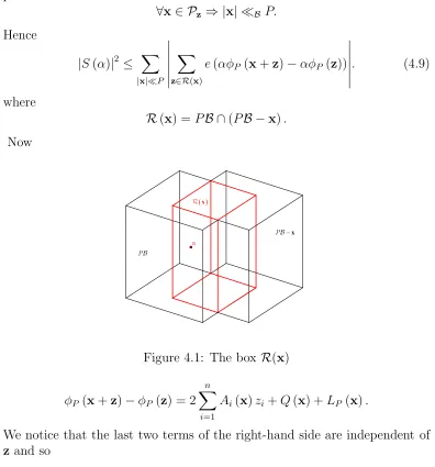
QzB={y∈Rn:z′ =z+y∈PB}. If

then, from Note 3.1, it follows that QzB ⊆ CP. If

R(y) =PB ∩QyB.

then, it is itself an n- box, with edges less than P in length and

|S(α)|2 ≤ X |y|< P

y_∈Zn

X

z∈R(y)∩Zn

e(α(ϕ(z+y)−ϕ(z)))

.

We call now

S′(α) = X z∈R(y)∩Zn

e(α(ϕ(z+y)₋ϕ(z))).

and we consider _|S′_(α)|2

.

Using the same argument as before, we have

|S′_(α)|2

≤ X

|x_|<P

X

z_∈S(x,y)∩Zn

e(α(φ(z+x+y)₋φ(z+x)₋φ(z+y) +φ(z)))

. where

S(x,y) =R(y)∩QxR(y). and

QxR(y) ={z∈Rn :z+x∈R(y)}. If

F (x,y,z) = (φ(z+x+y)−φ(z+x)−φ(z+y) +φ(z).

we have

F(x,y,z) =

n X i=1 n X j=1 n X k=1

c′i,j,kxiyjzk+η(x,y).

where η(x,y) does not depends 7 _{fromz. Hence}

F (x,y,z) =

n

X

j=1

Bj(x|y)zj +η(x,y).

It is well known that if k is any fixed integer and

then _X

m_∈A

e(mλ)≪minP,kλk−1 .

From this inequality we have

X

z∈S(x,y)∩Zn

e α

n

X

j=1

Bj(x|y)zj

!! ≪

n

Y

j=1

minP,_kαBj(x|y)k−1 .

Now using the last estimate in the estimate for|S2_{(α)|combined with Cauchy’s}

inequality, we have the result stated.

From now on, we write

S(α) =S(α, φ,_P, P). (3.20)

where_P is the parallelepiped in theRn

xspace obtained from the boxBin the

Rn_z space by means of the linear transformation z_→U(z) =xof Lemma 3.3

Definition 3.6. For a given set of bilinear forms

B=_{Bj :Rm×Rm →R, j = 1. . . n}.

we define

S∗(α,B, P) =Pm X

|x|<P

x_∈Zn

X

|y|<P

y_∈Zn

m

Y

j=1

minP,kαBj(x|y)k−1 . (3.21)

Lemma 3.5. If • ψ′

i :Rn→R, i= 1. . . s are the cubic polynomials of Lemma 3.3.

• Ci :Rni → R, i = 1. . . s their cubic parts (which depends only form

ni variables).

• Bi the set of bilinear forms associated to each Ci.

then

|S(α)|4 ≪P4n−4

s P i=1

ni

s

Y

i=1

Proof. Let _M the finite set of the representative solutions of the homoge-neous linear congruences (modd) as in Lemma 3.3 and let z0 ∈ M. We put

z = du+z0 where u ∈ Zn is an arbitrary vector with integer components. Substituting in (3.16) and (3.18) with _P in place of _R, we have

S(α) = X z0∈M



 X

u_∈B′ (z0)

e α

s

X

i=1

ψ′_i(du+z0)

! .

where

B′(z0) =u_∈Zn :u_∈d−1Qz0B .

and Qz0B is defined as in Lemma 3.4. We notice that For every z0 ∈ M there is an exponential sum of the form

X

u_∈B′ (z0)

e α

s

X

i=1

ψ_i′(du+z0)

!

. (3.23)

Hence S(α) is expressed as a finite sum of exponential sums of such a form. We apply to this sum the estimate given by Lemma 3.4. Since this estimate depends only on the cubic part of the polynomial, it is independent of z0. There is a minor discrepancy in that the box of summation depends on z0. Anyway the dependence is only by a bounded translation of vector

z0 and this trouble can be remedied by modifying the constants involved in

the conditions

|x| ≪P |y| ≪P.

We obtain (3.19) with bilinear forms which are associated with the cubic part of

ψ′(u) =

s

X

i=1

ψ′i(du+z0).

which is

C(u) =

s

X

i=1

Ci(du).

Since the cubic forms Ci are defined on disjoint sets, the bilinear forms fall

into sets of cardinality n1...ns and ms, where 8 ms = n − s

P

i=1

ni The ms

bilinear forms of the last set are identically zero. Accordingly, the right hand

8_{Of course not all the variables of the polynomial have to be present in its cubic part}

side of (3.19) can be factored. The factors areS∗_(α,B

i, P) where Bi is the set ofni bilinear forms associated with the cubic form Ci. We must observe

that there is also a factor of the kind AP4ms _{corresponding to the bilinear}

forms which are identically zero (being A a constant not depending on P) This proves the lemma.

3.8

The estimation of

S

(

α,

B

, P

)

if

h

(

C

) =

n

We introduce a parameter U to be specified later as well as the shortcut

L= logP. (3.24)

Now we shall reason indirectly and we develop some consequences if, for a givenα it is

S∗(α,B, P)> P4n_U−n_{. (3.25)}

We have the following

Lemma 3.6. If (3.25) holds and if NP =

n

(x,y)_∈Ae2P :kαBj(x|y)k < P−1 j = 1...n

o

. (3.26)

then

|NP)| ≫P2nU−nL−n. (3.27)

Proof. For everyx_∈Zn _let

NP(x) ={y∈Zn: (x,y)∈ NP}.

so that

|NP|=

X

|x|<P

|NP (x)|.

Let f(t) = t₋[t] denote the fractional part of any t _∈ R. Then, for any integer x and any integers r1...rn such that 0 ≤ rj < P j = 1...n the

inequalities _

   

P−1_{r1 ≤f(αB1(x|y))< P}−1_{(r1+ 1)}

...

P−1_r

n≤f(αBn(x|y))< P−1(rn+ 1).

cannot have more than |NP (x)| integer solutions y= (y1, . . . yn) such that

    

y1 ∈(a, b)

...

and b₋a= P. For if y′ _{is one solution of the system of inequalities and y} denotes the general solution, then

kαBj(x|y−y′)k< P−1 (j = 1. . . n).

and |y−y′_{|< P. Thus the number of possibilities for}