DISTANCE OF THE INITIAL WEIGHTS OF TREE PARITY MACHINE DRAWN FROM DIFFERENT DISTRIBUTIONS

(1)

137

Research Journal

Volume 9, No. 26, June 2015, pages 137–142

DOI: 10.12913/22998624/2380 Research Article

Received: 2015.04.12 Accepted: 2015.05.08 Published: 2015.06.01

DISTANCE OF THE INITIAL WEIGHTS OF TREE PARITY MACHINE

DRAWN FROM DIFFERENT DISTRIBUTIONS

Michał Dolecki1_{, Ryszard Kozera}1, 2

1_{The John Paul II Catholic University of Lublin, Konstantynów 1H, 20-708 Lublin, Poland, e-mail: michal.}

[email protected]

2_{Warsaw University of Life Sciences – SGGW, Nowoursynowska 159, 02-776 Warsaw, Poland, e-mail: ryszard.}

[email protected]; [email protected]

ABSTRACT

It is well-known that artificial neural networks have the ability to learn based on the provisions of new data. A special case of the so-called supervised learning is a mutual learning of two neural networks. This type of learning applied to a spe -cific networks called Tree Parity Machines (abbreviated as TPM networks) leads to achieving consistent weight vectors in both of them. Such phenomenon is called a network synchronization and can be exploited while constructing cryptographic key exchange protocol. At the beginning of the learning process both networks have initialized weights values as random. The time needed to synchronize both networks depends on their initial weights values and the input vectors which are also ran-domly generated at each step of learning. In this paper the relationship between the distribution, from which the initial weights of the network are drawn, and their com-patibility is discussed. In order to measure the initial comcom-patibility of the weights, the modified Euclidean metric is invoked here. Such a tool permits to determine the compatibility of the network weights’ scaling in regard to the size of the network. The proper understanding of the latter permits in turn to compare TPM networks of various sizes. This paper contains the results of the simulation and their discussion in the context of the above mentioned issue.

Keywords: neural networks, neurocryptography.

INTRODUCTION

Most of the stored or transmitted data often carry sensitive information and therefore it is vi -tal to protect them from potential threats [6]. Such a protection relates, among all, to data integrity or authorization of access and confidentiality of communication. One of the main goals here is to transfer the information so that it is impossible to decipher it by any unauthorized and unwanted person. In order to achieve this objective one re-sorts to various cryptographic algorithms [17].

The message containing information is here encrypted from the plain text to the ciphered text. According to the Kerckhoffs’s principle [14], most of the converting algorithms incorporate

additional input, i.e. the so-called cryptographic keys [1]. In this approach, the keys generating, distributing and storing methods become equally important issues. One of the options to generate the cryptographic keys is to invoke a well-known Diffie-Helmann protocol [14] which establishes a common key in an open communication chan -nel. However, another interesting approach stems from artificial intelligence, where artificial neural networks for cryptographic key exchange proce -dure [8, 11] can be applied. This method is based on the phenomenon of two networks’ synchro -nization by their mutual learning [10] described first by Kanter and Kinzel [9].

(2)

Advances in Science and Technology Research Journal Vol. 9 (26) 2015

availability of sample inputs supplemented with corresponding expected results of the network. These impulses are then sent to the taught net-work which in sequel calculates its output value. Next, the latter result is compared with the ex -pected result and the weights are modified ac -cordingly so that the outcome obtained from the network matches the expected results. In the two networks mutual learning variant is slightly different. First of all, no input-output set is con-structed at the preliminary step. Here, the input and output values are generated during the learn-ing process. Both networks receive the same in-puts and compute their output values. Then they exchange their respective calculated results. Both networks treat the received results of the counter-part network as the expected values and modify their weights according to the commonly adopted learning algorithm.

Upon imposing some restrictions on the net-works weight and their topological structure [15], which is called TPM network (the same for both networks), this learning procedure leads to the synchronization of the common weights in both networks. Such a process is called network syn -chronization in which a pair of adjusted weights change together yielding different but the same pairs of vectors representing in fact the desired cryptographic keys. An important fact is that learned/taught networks have a dynamic influ -ence on each other by exchanging their outputs. Evidently, the other “eavesdropping” network can intercept communications and gain access to the inputs and outputs of the self-taught net-works. However, this can be only passively ac -complished since the outputs of the third network are not fed-back to the synchronization process of the other two parties involved.

Consequently, as experimentally verified and statistically proven [10, 11] the passive net -work is not able to establish compatible weights as quickly as two actively synchronizing net -works. Such a phenomenon of establishing compatible network weights during their mutual learning can be therefore exploited in cryptog -raphy to construct relatively secure [12, 16] and computationally feasible key exchange protocol [2]. This new method based on TPM networks’ synchronization forms an alternative to the com -putationally difficult key exchange protocol problem which originally is tackled upon apply -ing various advanced NP-contemporary number theory techniques [14].

OBJECTIVE AND METHODOLOGY

The synchronization of TPM network is a stochastic process, which depends on the initial network weights and input values generated at each step of learning. This article discusses the impact of the distribution of the initial weights values drawn on their initial compatibility. The uniform and normal distributions with differ-ent parameters are applied and examined here in our examples with TPM networks having differ -ent topological parameters. For each variant of the distribution involved and TPM parameters fixed 5000 simulations of the selection of initial weights are carried out, which results in the total number of simulations amounting to 375 000. To evaluate the compatibility of the initial weight the cosine [15] and the modified Euclidean measures [4] are used.

TREE PARITY MACHINE

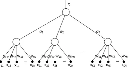
Tree Parity Machine (TPM) is a neural net -work used in cryptographic key exchange proto -col [10, 18]. It has specific topological structure and its operational modus vivendi somehow dif-fers from the conventional neural networks. In-deed, the TPM network consists of two layers of artificial neurons and in fact it is a feed-forward network. In the first layer it has K (K = 1, 2, …) artificial neurons constructed in accordance with the McCulloch – Pitts model [7, 13]. These neu -rons have not overlapping inputs, which imposes on TPM network a tree-like structure. In the sec -ond layer, the network has always one artificial neuron with a specific action, namely it multiplies the results of the first layer neurons. Lastly, the outcome of the output neuron is the result of the entire TPM network. To illustrate the above, a specific topology of the TPM structure is shown in the Figure 1.

(3)

139

Each neuron of the first layer has an inputs with values either –1 or 1. The synaptic weights are integers ranging within the interval from –L to L. The summation value of the neuron is calcu-lated without any bias, according to the following formula:

3

Fig. 1. TPM Structure.

Each neuron of the first layer has an

𝑁𝑁

inputs with values either -

1 or 1. The synaptic weights

are integers ranging within the interval from

−𝐿𝐿

to

𝐿𝐿

. The summation value of the neuron

𝑖𝑖

is

calculated without any bias, according to the

following formula:

𝜑𝜑

𝑖𝑖

= ∑

𝑁𝑁𝑖𝑖=1

𝑤𝑤

𝑖𝑖𝑖𝑖

𝑥𝑥

𝑖𝑖𝑖𝑖

.

The activation function

(acting on the summation)

of these neurons is a bipolar threshold

function

, which at the discontinuity is assume

d to return the value 1 for argument 0. Therefore

𝜎𝜎

𝑖𝑖

∈ {−1, 1}

, for

𝑖𝑖 = 1, 2, … , 𝐾𝐾

and the

whole TPM’s output as a product of

the first layer

neuron outputs is either

−1

or

1 . The

Tree Parity Machine has tree

-like structure and indicates

the parity of negative outputs of first layer neurons.

TPM network learning is performed according to the

algorithm, which de facto constitutes an

extension of the

network learning with the teacher.

More specifically, we deal here with

the

case of two networks

’

mutual learning

(and in fact teaching), in which both networks play

simultaneously a

role of a teacher and a role of a student

, interchangeably

. The two networks

involved

iteratively exchange their results as a teacher for the second network and modify

their weights as a student. The corresponding network weights are updated according to one

of three adopted methods: the anti-

Hebb

ian

rule, Hebb

ian rule or Random Walk rule:

1. Anti-

Hebbian rule

–

in this case neuron weights are modified if the outputs of both

networks are different. Weights’ modification complies here with the following

formula:

w_ij(t+1)= w_ij(t)Ǧxijσi

.

2. Hebbian rule

–

here weights are modified if the both TPM’s results are equal.

In this

method, weights are modified according to:

w_ij(t+1)= w_ij(t)+ xijσi

.

3. Random Walk rule

–

similar to normal Hebbian rule,

where mo

dification occurs only

if both results of the networks are equals. The respective

weights’ adjustment

s

depends here

only on the input signal

determined by the formula below

:

w_ij(t+1)= w_ij(t)+ xij

.

During entire learning

process only the

weights of these neurons are modified, for which the

outcome is equal to the result of the whole network. If the new weight value w

_ij(t+1)

is greater

than

𝐿𝐿

, it is replaced by

𝐿𝐿

and

similarly

if the weight value is less than

−𝐿𝐿

, it’s substituted by

– 𝐿𝐿

, accordingly

. As a result of such learning procedure, upon some number of steps,

the TPM

reaches a compatible weight values i.e. a

synchronization

state. If the weight

s’

modification is

carried out according to either

Hebbian

or Random Walk rule

the corresponding synchronized

weights have the same values. On the other hand if anti-

Hebbian method

is applied then these

values are opposite up

on synchronization is reached

.

The activation function (acting on the sum -mation) of these neurons is a bipolar threshold function, which at the discontinuity is assumed to return the value 1 for argument 0. Therefore,

3

Fig. 1. TPM Structure.

Each neuron of the first layer has an 𝑁𝑁

inputs with values either -

1 or 1. The synaptic weights

are integers ranging within the interval from

−𝐿𝐿

to

𝐿𝐿

. The summation value of the neuron

𝑖𝑖

is

calculated without any bias, according to the

following formula:

𝜑𝜑

𝑖𝑖

= ∑

𝑁𝑁𝑖𝑖=1

𝑤𝑤

𝑖𝑖𝑖𝑖

𝑥𝑥

𝑖𝑖𝑖𝑖

.

The activation function

(acting on the summation)

of these neurons is a bipolar threshold

function

, which at the discontinuity is assume

d to return the value 1 for argument 0. Therefore

𝜎𝜎

𝑖𝑖

∈ {−1, 1}

, for

𝑖𝑖 = 1, 2, … , 𝐾𝐾

and the

whole TPM’s output as a product of

the first layer

neuron outputs is either

−1

or

1 . The

Tree Parity Machine has tree

-like structure and indicates

the parity of negative outputs of first layer neurons.

TPM network learning is performed according to the

algorithm, which de facto constitutes an

extension of the

network learning with the teacher.

More specifically, we deal here with

the

case of two networks

’

mutual learning

(and in fact teaching), in which both networks play

simultaneously a

role of a teacher and a role of a student

, interchangeably

. The two networks

involved

iteratively exchange their results as a teacher for the second network and modify

their weights as a student. The corresponding network weights are updated according to one

of three adopted methods: the anti-

Hebb

ian

rule, Hebb

ian rule or Random Walk rule:

1. Anti-

Hebbian rule

–

in this case neuron weights are modified if the outputs of both

networks are different. Weights’ modification complies here with the following

formula:

w_ij(t+1)= w_ij(t)Ǧxijσi

.

2. Hebbian rule

–

here weights are modified if the both TPM’s results are equal.

In this

method, weights are modified according to:

w_ij(t+1)= w_ij(t)+ xijσi

.

3. Random Walk rule

–

similar to normal Hebbian rule,

where mo

dification occurs only

if both results of the networks are equals. The respective

weights’ adjustment

s

depends here

only on the input signal

determined by the formula below

:

w_ij(t+1)= w_ij(t)+ xij

.

During entire learning

process only the

weights of these neurons are modified, for which the

outcome is equal to the result of the whole network. If the new weight value

w_ij(t+1)

is greater

than

𝐿𝐿, it is replaced by 𝐿𝐿

and

similarly

if the weight value is less than

−𝐿𝐿

, it’s substituted by

– 𝐿𝐿, accordingly

. As a result of such learning procedure, upon some number of steps,

the TPM

reaches a compatible weight values i.e. a

synchronization

state. If the weight

s’

modification is

carried out according to either

Hebbian

or Random Walk rule

the corresponding synchronized

weights have the same values. On the other hand if anti-

Hebbian method

is applied then these

values are opposite up

on synchronization is reached

.

, for i = 1, 2, …, K and the whole TPM’s output as a product of the first layer neu -ron outputs is either –1 or 1. The Tree Parity Ma -chine has tree-like structure and indicates the par-ity of negative outputs of first layer neurons.

TPM network learning is performed accord -ing to the algorithm, which de facto constitutes an extension of the network learning with the teacher. More specifically, we deal here with the case of two networks’ mutual learning (and in fact teaching), in which both networks play simulta -neously a role of a teacher and a role of a student, interchangeably. The two networks involved it -eratively exchange their results as a teacher for the second network and modify their weights as a student. The corresponding network weights are updated according to one of three adopted meth-ods: the anti-Hebbian rule, Hebbian rule or Ran -dom Walk rule:

1) Anti-Hebbian rule – in this case neuron weights are modified if the outputs of both networks are different. Weights’ modification complies here with the following formula:

.

2) Hebbian rule – here weights are modified if the both TPM’s results are equal. In this meth -od, weights are modified according to:

.

3) Random Walk rule – similar to normal Heb -bian rule, where modification occurs only if both results of the networks are equals. The respective weights’ adjustments depends here only on the input signal determined by the for -mula below:

.

During entire learning process only the weights of these neurons are modified, for which the outcome is equal to the result of the whole

network. If the new weight value is

greater than L, it is replaced by L and similarly if the weight value is less than –L, it’s substituted by –L, accordingly. As a result of such learning procedure, upon some number of steps, the TPM reaches a compatible weight values i.e. a syn -chronization state. If the weights’ modification is carried out according to either Hebbian or Ran -dom Walk rule the corresponding synchronized weights have the same values. On the other hand if anti-Hebbian method is applied then these val -ues are opposite upon synchronization is reached.

Once two TPM networks are synchronized, they remain in this state regardless of their fur -ther learning and although each pair of respective weights of such networks changes along next iter -ations, they remain however equal in pairs. Only the network with an even number of neurons in the first layer may achieve the internal results configuration in which no weight will change in the neurons. This is possible when all hidden neu-rons have output equal to –1. There is therefore no internal neuron with the same result as the en-tire network so there is no weight modification.

KEY EXCHANGE PROTOCOL

The outlined above phenomenon of TPM syn -chronization can be used to construct the crypto -graphic key exchange protocol. More specifically, let A and B be two trusted parties who intend to establish the cryptographic key in order to en -crypt their further communication. The proposed protocol proceeds along the following steps: 0. Parties A and B determine (e.g. through an

open communication channel) the parameters

K, N and L describing the TPM network to -pology and the range of interval to which the weights of a learned networks belong. In addi-tion, both parties establish a common learning method. Of course, all such information is also available to the potential attacker (called here the third party).

1. Each of the parties (i.e. A and B) create their own TPM, with secretly randomly chosen re -spective weights wA_and_wB_.

2. Parties A and B obtain the same, publicly known input vector (also available to the third party) and calculate their corresponding TPM results τA_and_τB_.

(4)

140

4. Party A treats the result τB_{(received from B)}

as the expected result for its network, and B proceeds similarly with the value τA_(obtained

from A). Thus Parties A and B play simulte -neously the roles of teachers and students. 5. Both Parties A and B modify the weights of

the corresponding networks according to the mutually pre-selected learning method.

6. This process continues until the synchroniza -tion status is reached.

Once the two networks are synchronized, the entire learning process is completed, otherwise, it is continued upon returning to the step 2. The synchronization moment (i.e. adjusting the pairs of compatible weight vectors) can be accurately detected during the simulation program, which has access to the weight vectors of two networks involved. In practice the phenomenon of TPM network weights synchronization for crypto -graphic key exchange protocol yields weights which are in turn to be confidential. Therefore, the communication partners do not identify ex -actly a full synchronization moment. However, they can observe the exchanged results of both networks and once they coincide on different in -put vectors both TPM networks, such networks are considered as already synchronized. More specifically, sufficiently long exchange of con -sistent networks’ results for random inputs indi -cates that two networks have consistent weights [18]. We experimentally test here the answer to the question of time synchronization for different TPM parameters.

RESULTS

As it turns out, the time required to synchro -nize the TPM networks depends on their size. The latter involves the number of neurons in the hidden layer, the number of input values entering each of these neurons, the number of weights and finally the weight variation interval. Evidently, the number of input values is equal to the number of weights involved. All of the above-mentioned values are the network parameters K, N and L. In general, the larger the network is, the longer the synchronization takes [15]. As shown in the pre -vious works [5] the distribution of TPM network synchronization time has a characteristic left-hand histogram. The third quartile is nearly half of the longest observed synchronization time and this relationship remains valid for networks with

different topologies [3, 4]. Thus, it is important to focus on the fast synchronizations, which occur more frequently than long ones. Obviously, the synchronization time is crucial for the design of cryptographic key exchange protocol using TPM networks. TPM synaptic weight are assumed to be integers within the interval [–L, L]. At the be-ginning of synchronization procedure, both net -works weights are chosen randomly. An initial choice and randomly generated inputs determine the time of network learning. The closer to each other both weight vectors are, the more identical results both networks generate and consequently, they synchronize faster. On the other hand, any initial choice of distant weights may result in a long synchronization time increasing the risk of taking over the cryptographic key by the unde -sired third party.

The analysis of TPM networks with the ini -tial weights randomly chosen from the uniform distribution and normal distribution with differ-ent values of the standard deviation is performed in this paper below. Due to the symmetry of in -terval [–L, L], where the corresponding weights belong, the mean value of normal distribution is continuously equal to 0. The standard deviation s depends on the network parameter L and the cor-responding cases analyzed here include:

network synchronization time has a characteristic left

-hand histogram. The third quartile is

nearly half of the longest observed synchronization time and this relationship remains v

alid

for networks with different topologies [3,4]. Thus it is important to focus on the fast

synchronizations

, which occur more frequent

ly

than long ones.

Obviously, the

synchronization

time

is crucial for the design of cryptographic key exchange protocol using

TPM networks. TPM synaptic weight are

assumed to be integers within the interval

[– 𝐿𝐿, 𝐿𝐿]

.

At the beginning of synchronization

procedure

, both networks weights are chosen randomly

.

An initial choice and

randomly generated inputs determine the time of network learning. The

closer to each other both weight vectors are, the more both networks generate identical results

and

consequently synchronize faster. On the other hand any

initial choice of distant weights

may

result in a long

synchronization

time increasing the risk of taking over the

cryptographic

key by the undesired third party

.

The analysis of

TPM networks with the initial weights randomly chosen from the uniform

distribution and normal distribution with different values of the standard deviation is

performed in this paper below.

Due to the symmetry of interval

, where the

corresponding weights belong, the mean value of normal distribution is

continuously equal to

0. The standard deviation

𝑠𝑠

depends on the network parameter

𝐿𝐿

and the corresponding cases

analyzed

here include:

𝑠𝑠 ∈ {𝐿𝐿,

𝐿𝐿₂

,

𝐿𝐿₅

}

.

This distribution parameter has an impact o

n the frequency with which the weights’ values are

closer to 0 which in turn influences

the initial weight vectors compatibility.

We tested networks with

𝐾𝐾 = 3 and 𝑁𝑁 ∈ {11,50,100}.

Parameter

𝐿𝐿

is related to a standard

deviation

𝑠𝑠

and to the uniform and the normal distribution with

𝑠𝑠 = 𝐿𝐿

. Its value belongs here

to the following set

𝐿𝐿 ∈ {2,3,4, … ,10}

. For the normal distribution with

𝑠𝑠 =

𝐿𝐿₂

only even

values of

𝐿𝐿

are tested,

namely

𝐿𝐿 ∈ {2,4,6,8,10}

and for a standard deviation

𝑠𝑠 =

𝐿𝐿₅

only

values

for

𝐿𝐿

which are divisib

le by 5

are considered i.e.

𝐿𝐿 ∈ {5,10}

. This gives 75 possible variants

of parameters of

examined networks. E

ach network is tested with random initial weights draw

for 5000 times and in other experiment

with

5000 synchronizations. This

results in a total

number of 750000 cases.

In order to analyze

the initial weights c

ompatibility a

cosine function is applied

, originally

used by

Kanter et al [15] and

recently

used in

modified reversed Euclidean

distance [3,4]. The

cosine is calculated according formula:

𝜌𝜌

𝐴𝐴𝐴𝐴

_{= cos 𝜃𝜃 =}

𝑤𝑤𝐴𝐴∘𝑤𝑤𝐵𝐵 √𝑤𝑤𝐴𝐴_∘𝑤𝑤𝐴𝐴_√𝑤𝑤𝐵𝐵_∘𝑤𝑤𝐵𝐵

=

𝑤𝑤𝐴𝐴_∘𝑤𝑤𝐵𝐵 ‖𝑤𝑤𝐴𝐴_{‖∙‖𝑤𝑤}𝐵𝐵_‖

,

and the previous

ly

used Euclidean distance

reads as:

𝑑𝑑𝑑𝑑𝑠𝑠𝑑𝑑(𝐴𝐴, 𝐵𝐵)

𝑡𝑡

=

max

1≤𝑗𝑗≤𝑡𝑡𝑠𝑠𝑠𝑠𝑠𝑠𝑠𝑠ℎ𝑑𝑑𝑑𝑑𝑑𝑑𝑡𝑡(𝐴𝐴,𝐴𝐴)𝑗𝑗− 𝑑𝑑𝑑𝑑𝑑𝑑𝑡𝑡(𝐴𝐴,𝐴𝐴)𝑡𝑡 max

1≤𝑗𝑗≤𝑡𝑡𝑠𝑠𝑠𝑠𝑠𝑠𝑠𝑠ℎ𝑑𝑑𝑑𝑑𝑑𝑑𝑡𝑡(𝐴𝐴,𝐴𝐴)𝑗𝑗−1≤𝑗𝑗≤𝑡𝑡𝑠𝑠𝑠𝑠𝑠𝑠𝑠𝑠ℎmin 𝑑𝑑𝑑𝑑𝑑𝑑𝑡𝑡(𝐴𝐴,𝐴𝐴)𝑗𝑗

,

where

_{1≤𝑗𝑗≤𝑡𝑡}

max

𝑠𝑠𝑠𝑠𝑠𝑠𝑠𝑠ℎ

𝑑𝑑𝑑𝑑𝑠𝑠𝑑𝑑(𝐴𝐴, 𝐵𝐵)

𝑗𝑗

and

1≤𝑗𝑗≤𝑡𝑡

min

𝑑𝑑𝑑𝑑𝑠𝑠𝑑𝑑(𝐴𝐴, 𝐵𝐵)

𝑗𝑗

are assumed to be known. In this work

the distance is calculated in relation to the lowest and highest possible value

s, accordingly

.

The lowest distance is simply 0, whereas the biggest can be obtained when the corresponding

weights have opposite values

𝐿𝐿

and

−𝐿𝐿

. It can be calculated as follows:

max 𝑑𝑑𝑑𝑑𝑠𝑠𝑑𝑑(𝐴𝐴, 𝐵𝐵) = 2𝐿𝐿√𝐾𝐾𝑁𝑁

.

Table 1 presents results obtained for TPM

with the respective topological parameters 3-50-

L,

where

𝐿𝐿 ∈ {2,3,4, … ,10}

and the weights are drawn from the uniform and normal distributions

with the standard deviation

𝑠𝑠 = 𝐿𝐿

. The averag

e values of cosine and Euclidean

distance

depending on the

maximal possible distance

from 5000 randomly chosen initial weights

vectors are presented in the Table 1.

This distribution parameter has an impact on the frequency with which the weights’ values are closer to 0 which in turn influences the initial weight vectors compatibility.

We tested networks with K = 3 and N∈{11, 50, 100}. Parameter L is related to a standard de-viation s and to the uniform and the normal dis-tribution with s = L. Its value belongs to the fol-lowing set L∈{2, 3, 4, …, 10}. For the normal distribution with s = L/2 only even values of L

are tested, namely L∈{2, 4, 6, 8, 10} and for a standard deviation s=L/5 only values for L which are divisible by 5 are considered i.e. L∈{5, 10}. This gives 75 possible variants of parameters of examined networks. Each network is tested with random initial weights draw for 5000 times and in other experiment with 5000 synchronizations. This results in a total number of 750 000 cases.

(5)

141

5

network synchronization time has a characteristic left

-hand histogram. The third quartile is

nearly half of the longest observed synchronization time and this relationship remains v

alid

for networks with different topologies [3,4]. Thus it is important to focus on the fast

synchronizations

, which occur more frequent

ly

than long ones.

Obviously, the

synchronization

time

is crucial for the design of cryptographic key exchange protocol using

TPM networks. TPM synaptic weight are

assumed to be integers within the interval

.

At the beginning of synchronization

procedure

, both networks weights are chosen randomly

.

An initial choice and

randomly generated inputs determine the time of network learning. The

closer to each other both weight vectors are, the more both networks generate identical results

and

consequently synchronize faster. On the other hand any

initial choice of distant weights

may

result in a long

synchronization

time increasing the risk of taking over the

cryptographic

key by the undesired third party

.

The analysis of

TPM networks with the initial weights randomly chosen from the uniform

distribution and normal distribution with different values of the standard deviation is

performed in this paper below.

Due to the symmetry of interval

, where the

corresponding weights belong, the mean value of normal distribution is

continuously equal to

0. The standard deviation

𝑠𝑠

depends on the network parameter

𝐿𝐿

and the corresponding cases

analyzed

here include:

𝑠𝑠 ∈ {𝐿𝐿,

𝐿𝐿₂

,

𝐿𝐿₅

}

.

This distribution parameter has an impact o

n the frequency with which the weights’ values are

closer to 0 which in turn influences

the initial weight vectors compatibility.

We tested networks with

𝐾𝐾 = 3 and 𝑁𝑁 ∈ {11,50,100}.

Parameter

𝐿𝐿

is related to a standard

deviation

𝑠𝑠

and to the uniform and the normal distribution with

𝑠𝑠 = 𝐿𝐿

. Its value belongs here

to the following set

𝐿𝐿 ∈ {2,3,4, … ,10}

. For the normal distribution with

𝑠𝑠 =

𝐿𝐿₂

only even

values of

𝐿𝐿

are tested,

namely

𝐿𝐿 ∈ {2,4,6,8,10}

and for a standard deviation

𝑠𝑠 =

𝐿𝐿₅

only

values

for

𝐿𝐿

which are divisib

le by 5

are considered i.e.

𝐿𝐿 ∈ {5,10}

. This gives 75 possible variants

of parameters of

examined networks. E

ach network is tested with random initial weights draw

for 5000 times and in other experiment

with

5000 synchronizations. This

results in a total

number of 750000 cases.

In order to analyze

the initial weights c

ompatibility a

cosine function is applied

, originally

used by

Kanter et al [15] and

recently

used in

modified reversed Euclidean

distance [3,4]. The

cosine is calculated according formula:

𝜌𝜌

𝐴𝐴𝐴𝐴

_{= cos 𝜃𝜃 =}

𝑤𝑤𝐴𝐴∘𝑤𝑤𝐵𝐵 √𝑤𝑤𝐴𝐴_∘𝑤𝑤𝐴𝐴_√𝑤𝑤𝐵𝐵_∘𝑤𝑤𝐵𝐵

=

𝑤𝑤𝐴𝐴∘𝑤𝑤𝐵𝐵 ‖𝑤𝑤𝐴𝐴_{‖∙‖𝑤𝑤}𝐵𝐵_‖

,

and the previous

ly

used Euclidean distance

reads as:

𝑑𝑑𝑑𝑑𝑠𝑠𝑑𝑑(𝐴𝐴, 𝐵𝐵)

𝑡𝑡

=

max

1≤𝑗𝑗≤𝑡𝑡𝑠𝑠𝑠𝑠𝑠𝑠𝑠𝑠ℎ𝑑𝑑𝑑𝑑𝑑𝑑𝑡𝑡(𝐴𝐴,𝐴𝐴)𝑗𝑗− 𝑑𝑑𝑑𝑑𝑑𝑑𝑡𝑡(𝐴𝐴,𝐴𝐴)𝑡𝑡

max

,

where

max

𝑑𝑑𝑑𝑑𝑠𝑠𝑑𝑑(𝐴𝐴, 𝐵𝐵)

𝑗𝑗

and

min

𝑑𝑑𝑑𝑑𝑠𝑠𝑑𝑑(𝐴𝐴, 𝐵𝐵)

𝑗𝑗

are assumed to be known. In this work

the distance is calculated in relation to the lowest and highest possible value

s, accordingly

.

The lowest distance is simply 0, whereas the biggest can be obtained when the corresponding

weights have opposite values

𝐿𝐿

and

−𝐿𝐿

. It can be calculated as follows:

max 𝑑𝑑𝑑𝑑𝑠𝑠𝑑𝑑(𝐴𝐴, 𝐵𝐵) = 2𝐿𝐿√𝐾𝐾𝑁𝑁

.

Table 1 presents results obtained for TPM

with the respective topological parameters 3-50-

L,

where

𝐿𝐿 ∈ {2,3,4, … ,10}

and the weights are drawn from the uniform and normal distributions

with the standard deviation

𝑠𝑠 = 𝐿𝐿

. The averag

e values of cosine and Euclidean

distance

depending on the

maximal possible distance

from 5000 randomly chosen initial weights

vectors are presented in the Table 1.

and the previously used Euclidean distance reads as:

5

network synchronization time has a characteristic left-hand histogram. The third quartile is nearly half of the longest observed synchronization time and this relationship remains valid for networks with different topologies [3,4]. Thus it is important to focus on the fast synchronizations, which occur more frequently than long ones. Obviously, the synchronization time is crucial for the design of cryptographic key exchange protocol using TPM networks. TPM synaptic weight are assumed to be integers within the interval [– 𝐿𝐿, 𝐿𝐿]. At the beginning of synchronization procedure, both networks weights are chosen randomly. An initial choice and randomly generated inputs determine the time of network learning. The closer to each other both weight vectors are, the more both networks generate identical results and consequently synchronize faster. On the other hand any initial choice of distant weights may result in a long synchronization time increasing the risk of taking over the cryptographic key by the undesired third party.

The analysis of TPM networks with the initial weights randomly chosen from the uniform distribution and normal distribution with different values of the standard deviation is performed in this paper below. Due to the symmetry of interval [– 𝐿𝐿, 𝐿𝐿], where the corresponding weights belong, the mean value of normal distribution is continuously equal to 0. The standard deviation 𝑠𝑠 depends on the network parameter 𝐿𝐿 and the corresponding cases analyzed here include:

𝑠𝑠 ∈ {𝐿𝐿,𝐿𝐿₂,𝐿𝐿₅}.

This distribution parameter has an impact on the frequency with which the weights’ values are closer to 0 which in turn influences the initial weight vectors compatibility.

We tested networks with 𝐾𝐾 = 3 and 𝑁𝑁 ∈ {11,50,100}. Parameter 𝐿𝐿 is related to a standard deviation 𝑠𝑠 and to the uniform and the normal distribution with 𝑠𝑠 = 𝐿𝐿. Its value belongs here to the following set 𝐿𝐿 ∈ {2,3,4, … ,10}. For the normal distribution with 𝑠𝑠 =𝐿𝐿₂ only even values of 𝐿𝐿 are tested, namely 𝐿𝐿 ∈ {2,4,6,8,10} and for a standard deviation 𝑠𝑠 =𝐿𝐿₅ only values for 𝐿𝐿 which are divisible by 5 are considered i.e. 𝐿𝐿 ∈ {5,10}. This gives 75 possible variants of parameters of examined networks. Each network is tested with random initial weights draw for 5000 times and in other experiment with 5000 synchronizations. This results in a total number of 750000 cases.

In order to analyze the initial weights compatibility a cosine function is applied, originally used by Kanter et al [15] and recently used in modified reversed Euclidean distance [3,4]. The cosine is calculated according formula:

𝜌𝜌𝐴𝐴𝐴𝐴_{= cos 𝜃𝜃 =} 𝑤𝑤𝐴𝐴∘𝑤𝑤𝐵𝐵 √𝑤𝑤𝐴𝐴_∘𝑤𝑤𝐴𝐴_√𝑤𝑤𝐵𝐵_∘𝑤𝑤𝐵𝐵=

𝑤𝑤𝐴𝐴_∘𝑤𝑤𝐵𝐵 ‖𝑤𝑤𝐴𝐴_{‖∙‖𝑤𝑤}𝐵𝐵_‖, and the previously used Euclidean distance reads as:

𝑑𝑑𝑑𝑑𝑠𝑠𝑑𝑑(𝐴𝐴, 𝐵𝐵)𝑡𝑡=

max

,

where max

1≤𝑗𝑗≤𝑡𝑡𝑠𝑠𝑠𝑠𝑠𝑠𝑠𝑠ℎ𝑑𝑑𝑑𝑑𝑠𝑠𝑑𝑑(𝐴𝐴, 𝐵𝐵)𝑗𝑗 and1≤𝑗𝑗≤𝑡𝑡𝑠𝑠𝑠𝑠𝑠𝑠𝑠𝑠ℎmin 𝑑𝑑𝑑𝑑𝑠𝑠𝑑𝑑(𝐴𝐴, 𝐵𝐵)𝑗𝑗 are assumed to be known. In this work the distance is calculated in relation to the lowest and highest possible values, accordingly. The lowest distance is simply 0, whereas the biggest can be obtained when the corresponding weights have opposite values 𝐿𝐿 and −𝐿𝐿. It can be calculated as follows:

max 𝑑𝑑𝑑𝑑𝑠𝑠𝑑𝑑(𝐴𝐴, 𝐵𝐵) = 2𝐿𝐿√𝐾𝐾𝑁𝑁.

Table 1 presents results obtained for TPM with the respective topological parameters 3-50-L, where𝐿𝐿 ∈ {2,3,4, … ,10} and the weights are drawn from the uniform and normal distributions with the standard deviation 𝑠𝑠 = 𝐿𝐿. The average values of cosine and Euclidean distance depending on the maximal possible distance from 5000 randomly chosen initial weights vectors are presented in the Table 1.

where

5

network synchronization time has a characteristic left-hand histogram. The third quartile is

nearly half of the longest observed synchronization time and this relationship remains valid for networks with different topologies [3,4]. Thus it is important to focus on the fast

synchronizations, which occur more frequently than long ones. Obviously, the synchronization time is crucial for the design of cryptographic key exchange protocol using TPM networks. TPM synaptic weight are assumed to be integers within the interval [– 𝐿𝐿, 𝐿𝐿].

At the beginning of synchronization procedure, both networks weights are chosen randomly.

An initial choice and randomly generated inputs determine the time of network learning. The

closer to each other both weight vectors are, the more both networks generate identical results and consequently synchronize faster. On the other hand any initial choice of distant weights

may result in a long synchronization time increasing the risk of taking over the cryptographic key by the undesired third party.

The analysis of TPM networks with the initial weights randomly chosen from the uniform

distribution and normal distribution with different values of the standard deviation is

performed in this paper below. Due to the symmetry of interval [– 𝐿𝐿, 𝐿𝐿], where the

corresponding weights belong, the mean value of normal distribution is continuously equal to

0. The standard deviation 𝑠𝑠 depends on the network parameter 𝐿𝐿 and the corresponding cases

analyzed here include:

This distribution parameter has an impact on the frequency with which the weights’ values are

closer to 0 which in turn influences the initial weight vectors compatibility.

We tested networks with 𝐾𝐾 = 3and 𝑁𝑁 ∈ {11,50,100}. Parameter 𝐿𝐿 is related to a standard deviation 𝑠𝑠 and to the uniform and the normal distribution with 𝑠𝑠 = 𝐿𝐿. Its value belongs here to the following set 𝐿𝐿 ∈ {2,3,4, … ,10}. For the normal distribution with 𝑠𝑠 =𝐿𝐿₂ only even

values of 𝐿𝐿 are tested, namely 𝐿𝐿 ∈ {2,4,6,8,10} and for a standard deviation 𝑠𝑠 =𝐿𝐿₅only values for 𝐿𝐿 which are divisible by 5 are considered i.e. 𝐿𝐿 ∈ {5,10}. This gives 75 possible variants

of parameters of examined networks. Each network is tested with random initial weights draw

for 5000 times and in other experiment with 5000 synchronizations. This results in a total number of 750000 cases.

𝑤𝑤𝐴𝐴_∘𝑤𝑤𝐵𝐵 ‖𝑤𝑤𝐴𝐴_{‖∙‖𝑤𝑤}𝐵𝐵_‖,

and the previouslyused Euclidean distance reads as:

max

1≤𝑗𝑗≤𝑡𝑡𝑠𝑠𝑠𝑠𝑠𝑠𝑠𝑠ℎ𝑑𝑑𝑑𝑑𝑑𝑑𝑡𝑡(𝐴𝐴,𝐴𝐴)𝑗𝑗−1≤𝑗𝑗≤𝑡𝑡𝑠𝑠𝑠𝑠𝑠𝑠𝑠𝑠ℎmin 𝑑𝑑𝑑𝑑𝑑𝑑𝑡𝑡(𝐴𝐴,𝐴𝐴)𝑗𝑗 ,

where _{1≤𝑗𝑗≤𝑡𝑡𝑠𝑠𝑠𝑠𝑠𝑠𝑠𝑠ℎ}max 𝑑𝑑𝑑𝑑𝑠𝑠𝑑𝑑(𝐴𝐴, 𝐵𝐵)𝑗𝑗and_{1≤𝑗𝑗≤𝑡𝑡𝑠𝑠𝑠𝑠𝑠𝑠𝑠𝑠ℎ}min 𝑑𝑑𝑑𝑑𝑠𝑠𝑑𝑑(𝐴𝐴, 𝐵𝐵)𝑗𝑗are assumed to be known. In this work

the distance is calculated in relation to the lowest and highest possible values, accordingly.

The lowest distance is simply 0, whereas the biggest can be obtained when the corresponding

weights have opposite values 𝐿𝐿 and −𝐿𝐿. It can be calculated as follows:

Table 1 presents results obtained for TPM with the respective topological parameters 3-50-L,

where𝐿𝐿 ∈ {2,3,4, … ,10} and the weights are drawn from the uniform and normal distributions

with the standard deviation 𝑠𝑠 = 𝐿𝐿. The average values of cosine and Euclidean distance

depending on the maximal possible distance from 5000 randomly chosen initial weights

vectors are presented in the Table 1.

and

5

network synchronization time has a characteristic left-hand histogram. The third quartile is

nearly half of the longest observed synchronization time and this relationship remains valid for networks with different topologies [3,4]. Thus it is important to focus on the fast

synchronizations, which occur more frequently than long ones. Obviously, the synchronization time is crucial for the design of cryptographic key exchange protocol using TPM networks. TPM synaptic weight are assumed to be integers within the interval [– 𝐿𝐿, 𝐿𝐿].

At the beginning of synchronization procedure, both networks weights are chosen randomly.

An initial choice and randomly generated inputs determine the time of network learning. The

closer to each other both weight vectors are, the more both networks generate identical results and consequently synchronize faster. On the other hand any initial choice of distant weights

may result in a long synchronization time increasing the risk of taking over the cryptographic

key by the undesired third party.

The analysis of TPM networks with the initial weights randomly chosen from the uniform

distribution and normal distribution with different values of the standard deviation is

performed in this paper below. Due to the symmetry of interval [– 𝐿𝐿, 𝐿𝐿], where the

corresponding weights belong, the mean value of normal distribution is continuously equal to

0. The standard deviation 𝑠𝑠 depends on the network parameter 𝐿𝐿 and the corresponding cases

analyzed here include:

This distribution parameter has an impact on the frequency with which the weights’ values are

closer to 0 which in turn influences the initial weight vectors compatibility.

We tested networks with 𝐾𝐾 = 3 and 𝑁𝑁 ∈ {11,50,100}. Parameter 𝐿𝐿 is related to a standard

deviation 𝑠𝑠 and to the uniform and the normal distribution with 𝑠𝑠 = 𝐿𝐿. Its value belongs here

to the following set 𝐿𝐿 ∈ {2,3,4, … ,10}. For the normal distribution with 𝑠𝑠 =𝐿𝐿₂ only even

values of 𝐿𝐿 are tested, namely 𝐿𝐿 ∈ {2,4,6,8,10} and for a standard deviation 𝑠𝑠 =𝐿𝐿₅only values for 𝐿𝐿 which are divisible by 5 are considered i.e. 𝐿𝐿 ∈ {5,10}. This gives 75 possible variants

of parameters of examined networks. Each network is tested with random initial weights draw

for 5000 times and in other experiment with 5000 synchronizations. This results in a total number of 750000 cases.

𝑤𝑤𝐴𝐴_∘𝑤𝑤𝐵𝐵

‖𝑤𝑤𝐴𝐴_{‖∙‖𝑤𝑤}𝐵𝐵_‖,

and the previouslyused Euclidean distance reads as:

max

1≤𝑗𝑗≤𝑡𝑡𝑠𝑠𝑠𝑠𝑠𝑠𝑠𝑠ℎ𝑑𝑑𝑑𝑑𝑑𝑑𝑡𝑡(𝐴𝐴,𝐴𝐴)𝑗𝑗− 𝑑𝑑𝑑𝑑𝑑𝑑𝑡𝑡(𝐴𝐴,𝐴𝐴)𝑡𝑡

max

,

where max

1≤𝑗𝑗≤𝑡𝑡𝑠𝑠𝑠𝑠𝑠𝑠𝑠𝑠ℎ𝑑𝑑𝑑𝑑𝑠𝑠𝑑𝑑(𝐴𝐴, 𝐵𝐵)𝑗𝑗and 1≤𝑗𝑗≤𝑡𝑡min𝑠𝑠𝑠𝑠𝑠𝑠𝑠𝑠ℎ𝑑𝑑𝑑𝑑𝑠𝑠𝑑𝑑(𝐴𝐴, 𝐵𝐵)𝑗𝑗are assumed to be known. In this work

the distance is calculated in relation to the lowest and highest possible values, accordingly.

The lowest distance is simply 0, whereas the biggest can be obtained when the corresponding

weights have opposite values 𝐿𝐿 and −𝐿𝐿. It can be calculated as follows:

Table 1 presents results obtained for TPM with the respective topological parameters 3-50-L,

where𝐿𝐿 ∈ {2,3,4, … ,10} and the weights are drawn from the uniform and normal distributions

with the standard deviation 𝑠𝑠 = 𝐿𝐿. The average values of cosine and Euclidean distance

depending on the maximal possible distance from 5000 randomly chosen initial weights

vectors are presented in the Table 1.

are assumed to be known. In this work the dis-tance is calculated in relation to the lowest and highest possible values, accordingly. The lowest distance is simply 0, whereas the biggest can be obtained when the corresponding weights have opposite values L and –L. It can be calculated as follows:

5

network synchronization time has a characteristic left

-hand histogram. The third quartile is

nearly half of the longest observed synchronization time and this relationship remains v

alid

for networks with different topologies [3,4]. Thus it is important to focus on the fast

synchronizations

, which occur more frequent

ly

than long ones.

Obviously, the

synchronization

time

is crucial for the design of cryptographic key exchange protocol using

TPM networks. TPM synaptic weight are

assumed to be integers within the interval

.

At the beginning of synchronization

procedure

, both networks weights are chosen randomly

.

An initial choice and

randomly generated inputs determine the time of network learning. The

closer to each other both weight vectors are, the more both networks generate identical results

and

consequently synchronize faster. On the other hand any

initial choice of distant weights

may

result in a long

synchronization

time increasing the risk of taking over the

cryptographic

key by the undesired third party

.

The analysis of

TPM networks with the initial weights randomly chosen from the uniform

distribution and normal distribution with different values of the standard deviation is

performed in this paper below.

Due to the symmetry of interval

, where the

corresponding weights belong, the mean value of normal distribution is

continuously equal to

0. The standard deviation

𝑠𝑠

depends on the network parameter

𝐿𝐿

and the corresponding cases

analyzed

here include:

𝑠𝑠 ∈ {𝐿𝐿,

𝐿𝐿₂

,

𝐿𝐿₅

}

.

This distribution parameter has an impact o

n the frequency with which the weights’ values are

closer to 0 which in turn influences

the initial weight vectors compatibility.

We tested networks with

𝐾𝐾 = 3 and 𝑁𝑁 ∈ {11,50,100}.

Parameter

𝐿𝐿

is related to a standard

deviation

𝑠𝑠

and to the uniform and the normal distribution with

𝑠𝑠 = 𝐿𝐿

. Its value belongs here

to the following set

𝐿𝐿 ∈ {2,3,4, … ,10}

. For the normal distribution with

𝑠𝑠 =

𝐿𝐿₂

only even

values of

𝐿𝐿

are tested,

namely

𝐿𝐿 ∈ {2,4,6,8,10}

and for a standard deviation

𝑠𝑠 =

𝐿𝐿₅

only

values

for

𝐿𝐿

which are divisib

le by 5

are considered i.e.

𝐿𝐿 ∈ {5,10}

. This gives 75 possible variants

of parameters of

examined networks. E

ach network is tested with random initial weights draw

for 5000 times and in other experiment

with

5000 synchronizations. This

results in a total

number of 750000 cases.

In order to analyze

the initial weights c

ompatibility a

cosine function is applied

, originally

used by

Kanter et al [15] and

recently

used in

modified reversed Euclidean

distance [3,4]. The

cosine is calculated according formula:

𝜌𝜌

𝐴𝐴𝐴𝐴

_{= cos 𝜃𝜃 =}

𝑤𝑤𝐴𝐴∘𝑤𝑤𝐵𝐵

√𝑤𝑤𝐴𝐴_∘𝑤𝑤𝐴𝐴_√𝑤𝑤𝐵𝐵_∘𝑤𝑤𝐵𝐵

=

𝑤𝑤𝐴𝐴_∘𝑤𝑤𝐵𝐵 ‖𝑤𝑤𝐴𝐴_{‖∙‖𝑤𝑤}𝐵𝐵_‖

,

and the previous

ly

used Euclidean distance

reads as:

𝑑𝑑𝑑𝑑𝑠𝑠𝑑𝑑(𝐴𝐴, 𝐵𝐵)

𝑡𝑡

=

max

,

where

max

𝑑𝑑𝑑𝑑𝑠𝑠𝑑𝑑(𝐴𝐴, 𝐵𝐵)

𝑗𝑗

and

min

𝑑𝑑𝑑𝑑𝑠𝑠𝑑𝑑(𝐴𝐴, 𝐵𝐵)

𝑗𝑗

are assumed to be known. In this work

the distance is calculated in relation to the lowest and highest possible value

s, accordingly

.

The lowest distance is simply 0, whereas the biggest can be obtained when the corresponding

weights have opposite values

𝐿𝐿

and

−𝐿𝐿

. It can be calculated as follows:

max 𝑑𝑑𝑑𝑑𝑠𝑠𝑑𝑑(𝐴𝐴, 𝐵𝐵) = 2𝐿𝐿√𝐾𝐾𝑁𝑁

.

Table 1 presents results obtained for TPM

with the respective topological parameters 3-50-

L,

where

𝐿𝐿 ∈ {2,3,4, … ,10}

and the weights are drawn from the uniform and normal distributions

with the standard deviation

𝑠𝑠 = 𝐿𝐿

. The averag

e values of cosine and Euclidean

distance

depending on the

maximal possible distance

from 5000 randomly chosen initial weights

vectors are presented in the Table 1.

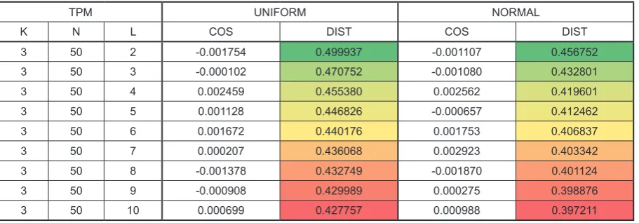
Table 1 presents the results obtained for TPM with the respective topological parameters 3-50-L, where L∈{2, 3, 4, …, 10} and the weights are drawn according to either uniform and normal distributions with the standard deviation s = L. The average values of cosine and Euclidean dis -tance depending on the maximal possible dis -tance from 5000 randomly chosen initial weights vectors are presented in the Table 1.

The tests performed for different TPM net -works yielded similar results. Within a fixed value of N, and upon increasing L the average distance of initial weights slightly decreases and the co -sine variations get close to zero without a visible regularity. Given the above observation, a further analysis focuses here on the Euclidean distance.

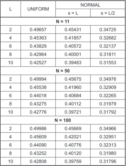
The choice of the specific distribution (from which the initial weights are drawn) results in the variation of distances between the initial drawn weights. In particular, the normal distribution renders a closer pairs of weights as opposed to

the uniform one. Table 2 shows the average dis-tances with respect to the maximal distance for 5000 random draws of the initial weights for all analyzed networks. Both uniform and normal dis -tributions (with standard deviation equal to L or L/2) are presented below.

Standard deviation of the used normal dis-tribution depends on the interval to which the weights of the tested network belong. The dis-tances between randomly generated weight vec -tors are scaled here to the maximal possible dis -tance appearing in a tested TPM network of a given fixed structure. Consequently, all generated results are similar and independent from different topological parameters.

Reducing the standard deviation leads to the further alignment of the initial weight vectors. In-deed, the similarity of the results described above permits to average them, which in turn is sum-marized in Table 3. The latter visibly indicates that the distance between the weights’ vectors is reduced in percentage.

In case when the weights are drawn according to a normal distribution the respective average distance decreases. For the standard deviations either L or L/2 or L/5, the corresponding calcu-lated distance is respectively 41.4%, 32.6% and 39.8% of the maximal distance and what is in -teresting this percentage occurs regardless of the size of the TPM network.

CONCLUSIONS

Having comparing the uniform and normal distributions with respect to the weights selection we observe that the latter favors the drawn weight values closer to the mean. Therefore, the distance between weight vector decreases. It is

interest-Table 1. Results for TPM with the topological parameters 3-50-L

TPM UNIFORM NORMAL

K N L COS DIST COS DIST

3 50 2 -0.001754 0.499937 -0.001107 0.456752

3 50 3 -0.000102 0.470752 -0.001080 0.432801

3 50 4 0.002459 0.455380 0.002562 0.419601

3 50 5 0.001128 0.446826 -0.000657 0.412462

3 50 6 0.001672 0.440176 0.001753 0.406837

3 50 7 0.000207 0.436068 0.002923 0.403342

3 50 8 -0.001378 0.432749 -0.001870 0.401124

3 50 9 -0.000908 0.429989 0.000275 0.398876

(6)

ing that expressing this distance, in relation to the maximal possible distance, yields similar results for networks with different parameters and thus renders the result independent from the size of the examined networks. The weights which are drawn closer to each other at the initial phase of the synchronization process should shorten the network synchronization time. This issue will be analyzed in a further research.

REFERENCES

1. Barker E., Barker W., Burr W., Polk W., Smid M.: Recommendation for key management – part 1: gen -eral (revision 3). National Institute of Standards and Technology Special Publication, 2012, 800–857. 2. Bisalapur S.: Design of an efficient neural key dis

-tribution center. International Journal of Artificial

Table 2. Distances for different TPMs and initial weights’ distributions

L UNIFORM NORMAL

s = L s = L/2

N = 11

2 0.49657 0.45431 0.34725

4 0.45363 0.41857 0.32682

6 0.43829 0.40572 0.32137

8 0.42964 0.40001 0.31811

10 0.42527 0.39483 0.31553

N = 50

2 0.49994 0.45675 0.34976

4 0.45538 0.41960 0.32909

6 0.44018 0.40684 0.32265

8 0.43275 0.40112 0.31979

10 0.42776 0.39721 0.31792

N = 100

2 0.49986 0.45669 0.34966

4 0.45609 0.42021 0.32951

6 0.44090 0.40776 0.32313

8 0.43252 0.40120 0.31980

10 0.42808 0.39759 0.31796

Table 3. Average distance for TPMs with different weights’ interval

N UNIFORM_[%] NORMAL [%]

L L/2 L/5

11 44.7 41.3 32.6 29.7

50 44.9 41.4 32.8 29.8

100 44.9 41.5 32.8 29.8

Intelligence & Applications, 2 (1), 2011, 60–69. 3. Dolecki M., Kozera R.: Threshold method of detect

-ing long-time TPM synchronization. Proceed-ings of the 12th_{International Conference on Computer}

Information Systems and Industrial Management Applications, Lecture Notes in Computer Science 8104, Springer – Verlag Berlin, 2013, 241-252. 4. Dolecki M., Kozera R., Lenik K.: The evaluation

of the TPM synchronization on the basis of their outputs. Journal of Achievements in Materials and Manufacturing Engineering, 57, 2013, 91–98. 5. Dolecki M., Kozera R.: Distribution of the Tree

Parity Machine synchronization time. Advances in Science and Technology Research Journal, 18, 2013, 20–27.

6. Gil A., Karoń T.: Analiza środków i metod ochrony systemów operacyjnych. Postępy Nauki i Techniki, 12, 2012, 149–168.

7. Hassoun M.: Fundamentals of Artificial Neural Networks. MIT Press, 1995.

8. Ibrachim S., Maarof M.: A review on biological in -spired computation in cryptology. Jurnal Teknologi Maklumat, 17(1), 2005, 90–98.

9. Kanter I., Kinzel W.: The theory of neural networks and cryptography. The Physics of Communication: Proceedings of the XXII Solvay Conference on Physics, 2002, 631–644.

10. Kanter I., Kinzel W., Kanter E.: Secure exchange of information by synchronization of neural net -works. Europhysics Letters, 57, 2002, 141–147. 11. Klein E., Mislovaty R., Kanter I., Ruttor A., Kinzel

W.: Synchronization of neural networks by mutual learning and its application to cryptography. Ad -vances in Neural Information Processing Systems, 17, MIT Press, Cambridge, 2005, 689–696. 12. Klimov A., Mityagin A., Shamir A.: Analysis of

neural cryptography, [In:] Y. Zheng (ed.), Advanc -es in Cryptology – ASIACRYPT 2002, Springer, 2003, 288–289.

13. McCulloch W.: A logical calculus of the ideas im -manent in nervous activity. Bulletin of Mathemati -cal Biophysics, 5, 1943, 115–133.

14. Menezes A., Vanstone S., Van Oorschot P.: Hand -book of Applied Cryptography. CRC Press, 1996. 15. Ruttor A.: Neural Synchronization and Cryptogra

-phy. PhD thesis, Wurzburg 2006.

16. Ruttor A., Kinzel W., Naeh R., Kanter I.: Genetic attack on neural cryptography. Physical Review E, 73(3), 2006, 036121.

17. Stokłosa J., Bilski T., Pankowski T.: Bezpieczeństwo danych w systemach informatycznych. PWN, 2001. 18. Volkmer M., Wallner S.: Tree parity machine