Post-processing scheme for modelling the lithospheric magnetic field

Solid Earth, 4, 105–118, 2013 www.solid-earth.net/4/105/2013/ doi:10.5194/se-4-105-2013

© Author(s) 2013. CC Attribution 3.0 License.

EGU Journal Logos (RGB)

Advances in

Geosciences

Open Access

Natural Hazards

and Earth System

Sciences

Open Access

Annales

Geophysicae

Open Access

Nonlinear Processes

in Geophysics

Open Access

Atmospheric

Chemistry

and Physics

Open Access

Atmospheric

Chemistry

and Physics

Open Access

Discussions

Atmospheric

Measurement

Techniques

Open Access

Atmospheric

Measurement

Techniques

Open Access

Discussions

Biogeosciences

Open Access Open Access

Biogeosciences

Climate

of the Past

Open Access Open Access

Climate

of the Past

Discussions

Earth System

Dynamics

Open Access Open Access

Earth System

Dynamics

Discussions

Geoscientific

Instrumentation

Methods and

Data Systems

Open Access

Geoscientific

Instrumentation

Methods and

Data Systems

Open Access

Discussions

Geoscientific

Model Development

Open Access Open Access

Geoscientific

Model Development

Hydrology and

Earth System

Sciences

Open Access

Hydrology and

Earth System

Sciences

Open Access

Discussions

Ocean Science

Open Access Open Access

Ocean Science

Solid Earth

Open Access Open Access

Solid Earth

Discussions

The Cryosphere

Open Access Open Access

The Cryosphere

Discussions

Natural Hazards

and Earth System

Sciences

Open Access

Discussions

Post-processing scheme for modelling the lithospheric magnetic field

V. Lesur1, M. Rother1, F. Vervelidou2, M. Hamoudi3, and E. Th´ebault2

1_{Helmholtz Centre Potsdam, GFZ German Research centre for Geosciences, Telegrafenberg 14473, Germany}

2_{Institut de Physique du Globe de Paris, Sorbonne Paris Cit´e, Univ. Paris Diderot, UMR7154 CNRS, 75005 Paris, France} 3_{Universit´e des sciences et de la technologie, 16111 Bab Ezzouar, El-Alia Alger, Algeria}

Correspondence to: V. Lesur ([email protected])

Received: 9 October 2012 – Published in Solid Earth Discuss.: 30 October 2012 Revised: 29 January 2013 – Accepted: 31 January 2013 – Published: 7 March 2013

Abstract. We investigated how the noise in satellite magnetic

data affects magnetic lithospheric field models derived from these data in the special case where this noise is correlated along satellite orbit tracks. For this we describe the satellite data noise as a perturbation magnetic field scaled indepen-dently for each orbit, where the scaling factor is a random variable, normally distributed with zero mean. Under this as-sumption, we have been able to derive a model for errors in lithospheric models generated by the correlated satellite data noise. Unless the perturbation field is known, estimating the noise in the lithospheric field model is a non-linear inverse problem. We therefore proposed an iterative post-processing technique to estimate both the lithospheric field model and its associated noise model. The technique has been successfully applied to derive a lithospheric field model from CHAMP satellite data up to spherical harmonic degree 120. The model is in agreement with other existing models. The technique can, in principle, be extended to all sorts of potential field data with “along-track” correlated errors.

1 Introduction

All geophysical data are contaminated by signals that cannot be easily described by models. These poorly parameterized contributions are often treated as errors and they most of the time exceed the pure instrumental noise. These kind of errors are particularly difficult to deal with because they are often correlated in space and/or time. Further they may not follow a Gaussian distribution. Yet properly handling the data errors is at the heart of the data interpretation process and it usu-ally requires their full statistical description – i.e. for a set of

discrete measurements, the knowledge of the full covariance matrix of the data errors.

Geopotential data – i.e. gravity and magnetic measure-ments – are no exception. For these types of data, the inverse problem that consists in finding the sources of the signals, is particularly ill-posed, and the proper statistical description of the data errors is necessary. Failing to do so may lead to false conclusions about the signal sources. From a practical point of view, scientists have been relatively successful in estimat-ing a priori the noise in gravity or magnetic data sets, how-ever correlations between errors have been mostly ignored. This is partly because, when known, the full covariance ma-trix for the data errors is generally so large that it cannot be handled easily, even on modern computers (but see for example Langel et al. (1989); Holme and Bloxham (1996); Rygaard-Hjalsted et al. (1997); Holme (2000), where corre-lated errors are accounted for in geomagnetism).

The effects of these correlation errors are obvious in air-borne, marine and satellite data. Typically, in all these type of surveys, the data are collected along linear paths and, af-ter processing, the correlation errors become apparent as off-sets between adjacent tracks. They then appear in maps and models as spurious anomalies, elongated in the direction of the tracks. An example of such an effect is shown in this manuscript for magnetic models derived from satellite data. The traditional way of dealing with this noise has been to perform a “leveling” of the data. In airborne geophysics, the approach mainly consists in deriving for each track a poly-nomial expression that is subtracted from the data such as to minimize data differences at the cross-over points (see for a review, e.g. Hamoudi et al., 2010). The method has also been adapted to satellite magnetic data. In such cases a large-scale field of external origin is fitted to a data set made of only

a few tracks. This allows us to successfully derive magnetic field models of the lithosphere to a relatively high degree. A well known example is theMFseries of models – e.g. Maus et al. (2008). However, the method, as applied to satellite data, has its drawbacks. The effects of its application have been carefully studied in Th´ebault et al. (2012) and it ap-pears that, depending on the way the method is applied, it can lead to significant distortions of the final model. How-ever, the weakest feature of this so-called “along-track fil-tering” approach is the impossibility to estimate how much the processing applied will distort the model. For this aspect, post-processing techniques are preferable.

So far, post-processing techniques have been developed and applied only to models derived from satellite gravity data – e.g. Kusche (2007). To the authors’ knowledge, such tech-niques have never been applied to magnetic models, although we should note the attempt to estimate the model covariance matrix in Lowes and Olsen (2004). In this manuscript we present and apply such a post-processing scheme for a model of the magnetic lithospheric field derived from ten years of CHAMP satellite data (Reigber et al., 2005). Although we are presenting this work from its application side, it has deeper roots: We investigated how typical noise correlated patterns leak, through a least squares fitting process, inside a magnetic model of the lithospheric field. This therefore lead to a model of the noise inside the lithospheric model. Once such a noise model is available, numerous post-processing schemes are possible; we just applied one specific approach to show that the noise model we obtained is relevant. The fi-nal resulting model of the lithospheric field is nonetheless of high quality and compares well with other recently re-leased models (e.g. MF7 that is not published but the MF6 is presented in Maus et al. (2008); CHAOS-4; Olsen et al., 2010b) as well as older models (see for a review Th´ebault et al., 2010).

The manuscript is organized as follows. In the next section we set the hypothesis and approximations, derive the general expression for the noise model and give examples of possi-ble noise, depending on the characteristic of the perturbation magnetic field in the data. In the third section we describe in detail the two-step process towards the final lithospheric field model; the resulting model is then discussed. We conclude in the last section.

2 The lithospheric noise model

In this section we present a noise model for a lithospheric model estimated from a set of radial magnetic data. We choose to present this case only in the main part of this manuscript as the equations are relatively simple to derive. The description for the usual case where the lithospheric model is obtained from the three components of a magnetic data set is given in Appendix A.

2.1 Theory

We consider a magnetic data set made of radial component readings along a single CHAMP satellite half-orbit during night-time periods. For simplicity we will assume that a track follows a meridian – i.e. it corresponds to a single longi-tude value – which is a reasonable approximation for near-polar orbiting satellites. Several magnetic field sources are contributing to these data (Hulot et al., 2007), typically the core and lithospheric fields, the ionospheric and magneto-spheric fields, and the fields generated by field aligned cur-rents. Other contributions exist, as the field induced in the conductive layers of the Earth, but they are of much weaker amplitudes. Mathematical models are available for all these contributions and can be subtracted from the data, leaving residuals due mainly to the limited precision of these mod-els. In particular, the description of the external field is not very accurate and the residuals obtained along that half-orbit track contain relatively long wavelengths. We assume that these residuals are well approximated by the radial compo-nent of an external magnetic field model that does not present time dependencies. It is hereafter named as the perturbation field and can be written

Brp(θ, φ, r)= − N

X

n,k (r

a) n−1_n k

nYnk(θ, φ), (1)

where_nkis the Gauss coefficient of degreenand orderk,a=

6371.2 km is the Earth’s reference radius, andY_nk(θ, φ)are the Schmidt semi-normalized spherical harmonics (SHs). We use throughout this manuscript the convention that negative orders, k <0, are associated with sin(|k|φ)terms whereas null or positive orders, k≥0, are associated with cos(kφ) terms.

We consider also a model of the radial component of a magnetic field of internal origin with no temporal dependen-cies. This model becomes below the lithospheric noise model we want to derive:

˜

Bri(θ, φ, r)= L

X

l,m (a

r)

l+2_(l+1)g˜m

l Ylm(θ, φ). (2)

It is not possible to separate external field contributions from internal field contributions for data collected along a sin-gle meridian (Olsen et al., 2010a) – i.e. a sinsin-gle half-orbit – hence we can fit by least-squares the residuals defined in Eq. (1) with the lithospheric model given in Eq. (2) and find a non-zero solution. This least-squares solution is found by minimizing the functional

8j=

X

i

wi| ˜Bri(θi, φj, r)−Brp(θi, φj, r)|2, (3)

whereθi are sampling points along the half-orbit,φj is the

Over 10 yr, the CHAMP satellite has collected data along a large numberMof half-orbits. We assume now that for each orbit the perturbation field model defined by Eq. (1) is scaled by a numberηj and that all orbits are at the same radiusr.

This latter point is clearly a strong approximation but there is no obvious way to avoid it. Again, these external field con-tributions can be interpreted as a field of internal origin. To estimate this field, the functional we have to minimize is 8=X

i,j

wi| ˜Bri(θi, φj, r)−ηj·Brp(θi, φj, r)|2. (4)

Minimizing8for the Gauss coefficientsg˜m_l leads to a system of equations:

AtAg˜=Atb (5)

where g˜= [ ˜g_lm]_{l,m}. The matrix product AtA is derived

from Eqs. (2), (4) and the elements of this product associ-ated with the degrees and ordersl, l0, m, m0can be written

{AtA}_l,m,l0_,m0=M(

a r)

l+l0₊₄

(l+1)(l0+1)hP_l|m|, P|m

0_|

l0 i5mm0 (6)

where the producthP_lm, P_lm00iis defined by

hP_lm, P_lm0 0i = X

i

wiPlm(cosθi) Pm

0

l0 (cosθi). (7)

The variable5mm0has been introduced to cover three cases:

5mm0=  



1 M

PM

i=1cosmφi sin|m0|φi ifmm0<0 1

M

PM

i=1cosmφi cosm0φi ifm≥0, m0≥0 1

M

PM

i=1sin|m|φi sin|m0|φi ifm <0, m0<0,

(8) and is symmetric relative to its subscripts – i.e. 5mm0=

5m0_m.

The elements of the right-hand side vector of Eq. (5) are

{Atb}_l,m= −M

N

X

n,k

(a r)

l−n+3_n(l+1)hP|k| n , P

|m| l i

k

nχmk. (9)

Depending on the sign of the ordersmandk,χ_mk takes the following values:

χ_mk =

 



1 M

PM

i=1cosmφi coskφi ηi ifm, k≥0 1

M

PM

i=1cosmφi sin|k|φi ηi ifmk <0 1

M

PM

i=1sin|m|φi sin|k|φi ηi ifm, k <0.

(10)

As for5mm0, it is symmetric relative to its subscripts:χk

m=

χ_km. We note at this point that it is important to have theηi

constant along half-orbits; otherwise, the summations over latitudes and longitudes could not be separated.

For very large number M of orbits uniformly dis-tributed along longitudes, the quantity 5mm0 tends to aδ

-function – i.e.5mm0 '(1

2+ 1

2δm0)δmm0. Further, by setting the weights wi to wi=sinθi and assuming that the

sam-pling points are evenly spaced over the full meridian, we have

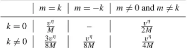
Table 1. Estimated variance ofχ_mk

m=k m= −k m6=0 andm6=k

k=0 v_Mη – ₂v_Mη

k6=0 3₈v_Mη ₈v_Mη ₄v_Mη

hP_l|m|, P_l|0m|i =

4−2δm0

2l+1 δll0. The value given to the weightsw_i

is less important than insuring the orthogonality of the Leg-endre functions through the producthP_l|m|, P_l|0m|i. This is also

what a modeler tries to acheive when building a lithospheric magnetic field model from real data. However, assuming that both5mm0 andhP|m|

l , P

|m|

l0 ican be regarded asδ-functions,

it is easy to see from Eq. (6) that the product matrix AtA is

diagonal. Now turning to Eqs. 9, 10, if theηi form a set of

uncorrelated random variables, theχ_mk are also random vari-ables with zero mean.

The Gauss coefficients for the lithospheric noise model in Eq. (2) are then obtained by combining Eqs. (5), (6) and (9):

˜ gm_l = −

N

X

n,k (r

a)

l+n+1_n2l+1 2l+2hP

|k|

n , P

|m|

l i

k

nχmk. (11)

They correspond to the noise in a lithospheric field model that would be generated by un-modelled external fields in the radial component of magnetic data. Similarly, it is straightforward to find the noise in a lithospheric field model (i.e. static internal field model) generated by a perturbation field of internal origin. This case is relevant for signals gen-erated in the lower E-region ionosphere (e.g. at 110 km al-titude) when data are acquired at satellite altitudes. Other possible sources for this type of noise are the un-modelled induced fields generated in the conductive layers of the Earth by rapid variations of the external fields. It gives the follow-ing result:

˜ gm_l =

N

X

n,k (r

a)

l−n_(n+1)2l+1

2l+2 hP

|k|

n , P

|m|

l iı k

nχmk, (12)

whereı_nkare the Gauss coefficients for the ionospheric and/or induced field models.

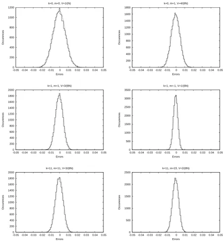
In order to understand the behaviour of the lithospheric noise model, it is important to have an estimate of the prob-ability density function of the random variableχ_mk. Assum-ing the random variableηis normally distributed with vari-ancevη, thenχ_mk appears to be also normally distributed. The set ofχ_mk are uncorrelated with the exception thatχ_mk =χ_km. Further, theχ_mk have a variancevχ that depends onvη, the number of half-orbitsM, and the orders kandm. Possible values of the variancevχ are given in Table 1. These vari-ances have been derived from numerical experiments involv-ing 20 000 independent realizations of the random variables χ_mk calculated from the same number of uniformly distributed

orbits. They can also be estimated analytically as shown in Appendix B. Figure 1 presents the histograms for several val-ues ofmandk.

In the remaining parts of this section we consider only the noise model given by Eq. (12). The general behaviour of the noise characterized by Eqs. (12) and (11) is basically the same. In particular, they have the same dependence rela-tive to the degreel. These two noise models are only relevant for the cases where the radial components of vector data are used. The way the noise propagates in a lithospheric model is different if the three components of the vector data are fit-ted. The corresponding equations for that case are relatively complex and given in Appendix A.

The noise model defined in Eq. (2) hasL(L+2) parame-ters – i.e.L(L+2)Gauss coefficients. This number reduces toN (N+2)Gauss coefficientsı_nkwith(2N+1)(2L+1)−

2N2random variablesχ_mk through Eq. (12). For small values ofN – e.g.N=10 – there is a very significant reduction of number of parameters, but Eq. (12) is non-linear.

2.2 Examples

In order to understand the main characteristics of the noise model defined by Eqs. (2) and (12), we present in this sec-tion the results of forward modelling calculasec-tions for a given choice of Gauss coefficientsık_nand one realization of the set of random variablesχ_mk. The productshPn|k|, P

|m|

l i are

cal-culated numerically. These products are relatively difficult to estimate accurately as theP_lm(x)functions are oscillatory. However, an adaptive Gaussian quadrature (Piessens et al., 1983; Kahaner et al., 1989) was ultimately chosen as it gave the best results.

2.2.1 Dipole perturbation field

For this first example we use a simple model for the per-turbation field of internal origin made of a single spherical harmonic n=1, k=1. Specifically, we set ı₁1=1 nT and ı_nk=0 nT for{n, k} 6= {1,1}. This type of noise in satellite data could result from a poor modelling of the field induced by a large-scale external field in the conductive layers of the Earth. In that case Eq. (12) reduces to

˜ gm_l =(r

a)

l−1₂2l+1 2l+2 hP

|1|

1 , P

|m|

l iı 1 1χ

1

m, (13)

and the noise in the radial component of the field of internal origin is

˜

Bri(θ, φ, r0)=ı112( a r0)

3 ₍₁₄₎

L

X

l,m (r

r0)

l−1(l+1)(2l+1) (2l+2) hP

|1|

1 , P

|m|

l iχ

1

mYlm(θ, φ),

where r0 is the modelling radius that is set to r0=a=

6371.2 km in this example. As the observation radiusris ex-pected to be larger than the modelling radius, the short

wave-lengths dominate the model due to the ratio _rr0 raised to the

powerl−1 in the right-hand side of Eq. (14).

In Fig. 2, the model defined by Eq. (14) is mapped for the model coefficientı₁1=1 nT, an observation radius at 300 km altitude (r=6671.2 km) and the random variablesχ_m1 with variances defined in Table 1 using vη=M. The maximum SH degree involved isL=120. We observe that the noise model is symmetric relative to the Equator, vanishes at the poles, and is made of east–west oscillating anomalies typical of the noise in lithospheric field model derived from satel-lite data. We note that these characteristics are independent from the sign of the SH orderkas only the random variable χ_mk depends on this sign in Eq. (14). The obtained symme-try of the model is due to the product hP₁|1|, P_l|m|i, which vanishes if the Legendre functionP_l|m| is anti-symmetric – i.e. l− |m| is odd. An anti-symmetric model, vanishing at the Equator but not at the poles, would have been obtained ifı₁0=1 nT would have been chosen in place of ı1₁=1 nT. These symmetry/anti-symmetry characteristics are specific to models derived from the radial component alone. It can be seen in Appendix A that these characteristics are lost when a noise model is obtained from the three vector components.

The power spectrum of the model calculated at r0=

6371.2 km is also plotted in Fig. 2. It presents some vari-ability due to the use of a single SH in Eq. (13). Nonetheless, the behaviour is generally along a (_rr0)2l trend as it would

be expected for a white noise at satellite altitude. Although the small wavelengths overshadow the larger wavelengths, the latter are also present in the noise model. It is clear that any magnetic field model derived from satellite data is con-taminated by such noise at all wavelengths unless pertinent processing steps are applied.

2.2.2 Auroral electrojet and field aligned currents

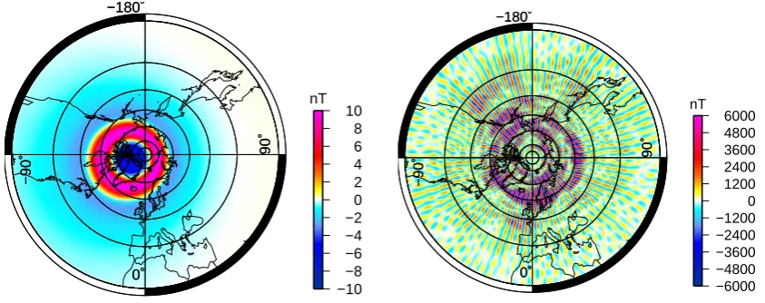
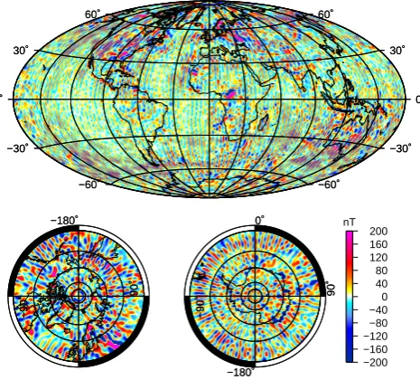
Another expected source of noise in satellite data is associ-ated with auroral electrojet and / or associassoci-ated field-aligned currents. We do not aim at a precise description of the distur-bance field but just consider the radial component of a per-turbation field of internal origin, mapped in Fig. 3, left, and defined by

Brp(θ, φ, r)= N

X

n,k (a

r)

n+2_(n+1)ık

nYnk(θ, φ). (15)

0 200 400 600 800 1000 1200

-0.05 -0.04 -0.03 -0.02 -0.01 0 0.01 0.02 0.03 0.04 0.05

Occurences

Errors k=0, m=0, V=1/(N)

0 200 400 600 800 1000 1200 1400 1600 1800

-0.05 -0.04 -0.03 -0.02 -0.01 0 0.01 0.02 0.03 0.04 0.05

Occurences

Errors k=0, m=1, V=4/(8N)

0 200 400 600 800 1000 1200 1400 1600 1800 2000

-0.05 -0.04 -0.03 -0.02 -0.01 0 0.01 0.02 0.03 0.04 0.05

Occurences

Errors k=1, m=1, V=3/(8N)

0 500 1000 1500 2000 2500 3000 3500

-0.05 -0.04 -0.03 -0.02 -0.01 0 0.01 0.02 0.03 0.04 0.05

Occurences

Errors k=1, m=-1, V=1/(8N)

0 200 400 600 800 1000 1200 1400 1600 1800 2000

-0.05 -0.04 -0.03 -0.02 -0.01 0 0.01 0.02 0.03 0.04 0.05

Occurences

Errors k=11, m=11, V=3/(8N)

0 500 1000 1500 2000 2500

-0.05 -0.04 -0.03 -0.02 -0.01 0 0.01 0.02 0.03 0.04 0.05

Occurences

Errors k=11, m=23, V=2/(8N)

Fig. 1.

Histograms of the random variable

χ

for several values of

k

and

m. Is also plotted the dashed curve

M_·S √

2πvχ

exp

{−

e

/(2v

)

}

where

S

is the histogram step length.

Table 1.

Estimated variance of

χ

m

=

k

m

=

−

k

m

̸

= 0

and

m

̸

=

k

k

= 0

-

k

̸

= 0

20

Fig. 1. Histograms of the random variableχ_mk for several values ofkandm. Also plotted is the dashed curve√M·S

2π vχexp{−e

2_/(2vχ_)}where

Sis the histogram step length andethe error.

localized in latitudes as it basically vanishes in the Southern Hemisphere. However, it seems that the noise is propagating over all longitudes. The power spectrum of the model has es-sentially the same characteristic as in the previous example.

The results of this example have to be analysed with some caution since real satellite orbits deviate from the exact polar direction at high latitudes. Nonetheless, we take from these

results that there is no need to describe precisely the longitu-dinal dependence of the perturbation field to obtain a realistic noise model. Therefore, in Eq. (12), the range of SH orderk can be restricted to small values – e.g. kmax=2 – even if the maximum SH degree in the model remains large – e.g. N=30. This will reduce even further the number of param-eters needed to describe the noise model.

−60˚ −60˚

−30˚ −30˚

0˚ 0˚

30˚ 30˚

60˚ 60˚

−60˚ −60˚

−30˚ −30˚

0˚ 0˚

30˚ 30˚

60˚ 60˚

−180˚

−90˚

0˚

90˚

−180˚

−90˚

0˚

90˚

−180˚

−90˚

0˚

90˚

−180˚

−90˚

0˚

90˚

−6000 −4800 −3600 −2400 −1200 0 1200 2400 3600 4800 6000 nT

0.1 1 10 100 1000 10000 100000 1e+06

0 20 40 60 80 100 120

(nT)

2

SH degree

Fig. 2. Left: Mapping atr0=6371.2 km of the model defined in Eq. (14) whereı₁1=1,r=6671.2 km – i.e. 300 km altitude – and the random variablesχ_m1 have a variance defined in Table 1 usingvη=M. Right: Associated power spectrum. The dashed line is proportional to(_rr0)2l.

−180˚

−90˚

0˚

90˚

−180˚

−90˚

0˚

90˚

−10 −8 −6 −4 −2 0 2 4 6 8 10 nT

−180˚

−90˚

0˚

90˚

−180˚

−90˚

0˚

90˚

−6000 −4800 −3600 −2400 −1200 0 1200 2400 3600 4800 6000 nT

Fig. 3. Mapping atr0=6371.2 km of the field of internal origin (left) and the resulting noise model (right). The data acquisition radius has been set tor=6671.2 km – i.e. 300 km altitude – and the random variablesχ_mk have the variances defined in Table 1 with the ratiov_Mη set to 1.

3 Application to magnetic models of the lithosphere

We are now using the results presented in the previous sec-tion to derive a model of the magnetic field generated in the lithosphere from real CHAMP satellite data. The pro-cess we applied to calculate such a model is in two stages. First, we estimate a rough lithospheric field model from satel-lite data using a usual approach and a straightforward least-squares process (e.g. Lesur et al., 2008). Second, in the post-processing stage, we co-estimate a new lithospheric field model and a model of the noise where the output model of the first stage is used as data. The final results depend on the

processes applied during the two stages and therefore both are described in independent subsections below.

In order to avoid confusion between the different models, we use the following notations for the fields and Gauss coef-ficients:

– the noisy lithospheric model, output of the first stage, is

denoted using aˆ.– e.g.Bˆifor the magnetic field vector,

– the lithospheric field model output of the

Table 2. Thresholds and misfit values obtained when estimating_Bˆ_i

from selected satellite data. Mid- and low-latitudes are defined by magnetic latitudes in between±55 deg. Values are given in nT.

Mid- and low-latitudes High latitudes

X_SM Y_SM Z_SM X_SP Y_SP Z_SP

Threshold 9.0 8.5 10.5 36 27 36 Misfit 2.47 2.30 2.53 13.52 10.79 10.49

– the noise model is denoted, in the same way as in the

previous section, using a˜.– e.g.B˜i.

3.1 First stage: Data set, data selection, model parameterization and model estimation

Three component vector magnetic readings acquired during the ten years of the German CHAMP satellite mission are used. The data are selected for night-time periods and mag-netically quiet days, in the same way as data are selected for the GRIMM series of core field models (Lesur et al., 2008, 2010). However, here the three components of the vector data are used and data in single star camera mode are rejected, whereas in the GRIMM selection scheme only the X and Y SM components are selected at mid- and low-latitudes. A core field model and a model of the large-scale external field with its internally induced counterpart are subtracted from these data, leaving mainly the contributions from the litho-sphere and the noise. The core field model and external field models used are resulting from the derivation of GRIMM-3 (Lesur et al., 2011), but this is not seen as an important point in the processing; another core field model would have been possible – e.g. CHAOS-4 (Olsen et al., 2010b).

Next, a first lithospheric field model up to SH degree 60 is derived, but our aim here is to reject outliers. The data cor-responding to residuals larger than 3 times the standard de-viation are rejected. The value of the threshold, for each data type, is given in Table 2. This selection process is known to potentially strongly affect the final lithospheric field model. At mid- and low-latitudes only few data are rejected, and those rejected data do not present clusters; no major diffi-culties are therefore expected there. At high latitudes, how-ever, a large amount of data are rejected and it is not possi-ble to assess at this point if magnetic anomalies are erased or minimized there. We checked, however, that outside the polar gaps due to the satellite orbits, the final data density at satellite altitude is everywhere large enough to allow for a lithospheric field model to be estimated up to SH degree 120. In order to avoid spurious oscillations of the lithospheric model, further vertical down component data values were added over the polar gaps at an altitude of 6371.2 km. The data values were arbitrarily set to zero, and the associated weights for the inversion process were adjusted such that the

lithospheric field model remained smooth while the misfit to the original satellite data stayed unchanged. We have tested other possible approaches, but the one we used gave the best results. One could alternatively use vertical down component values derived from aeromagnetic maps.

The data set resulting from this selection process still con-sists in some 5 014 325 data values. A model of the litho-sphere magnetic field, defined by Eq. (16) below, was fitted through a simple least-squares process to the data. The data weights are set to mimic a homogeneous data repartition and therefore depend only on the inverse of the data density.

ˆ

Bi(θ, φ, r)= −∇ "

a L=120

X

l,m (a

r) l+1_gˆm

l Ylm(θ, φ)

#

. (16)

The power spectrum at the Earth surface of the resulting lithospheric field model is presented in Fig. 4, left side, to-gether with the power spectrum of the CHAOS-4 model. Both models present very similar spectra up to SH degree 60 or 65. Our model presents slightly less power around de-gree 70, possibly due to the selection technique used. Above SH degree 85, CHAOS-4 spectrum is strongly minimized, whereas our model presents a spectrum rising to high values, evidence of the predominance of noise in the model at these SH degrees. The final misfits to the data are given in Table 2. The vertical down component of the model – i.e. theZ component – is mapped at 300 km above the Earth surface in Fig. 4, right side. At this altitude the long wavelength lithospheric signal dominates but the noise is clearly visible, mainly over oceans, as elongated anomalies in the north– south direction – e.g. to the south of Australia. We point out that there are strong correlations between the estimated Gauss coefficients of the model and therefore the model can-not be truncated at an arbitrary degree without introducing artefacts.

3.2 Second stage: model post-processing

The post-processing part consists in fitting a model of the magnetic field generated in the lithosphere together with the model of noise to a 300 km altitude map of the vertical down component of the field model Bˆi(θ, φ, r)(see Fig. 4). The noise modelB˜iwe used is derived in Appendix A and is pa-rameterized by the variableχ_mk and the Gauss coefficients of the perturbation modelı_nk. This inverse problem that consists in fitting the noise model and the lithospheric field model to

ˆ

BZivalues presents some difficulties that are described first;

results are given in a second subsection.

3.2.1 Inverse problem

We map the vertical down component of the magnetic field modelBˆi(θ, φ, r)at 29 161 positions on a Gauss–Legendre grid at r=300 km altitude. These data values are related to the Gauss coefficients g_lm of the field model Bi by the

1 10 100 1000

20 40 60 80 100 120

(nT)

2

SH degree

−60˚ −60˚

−30˚ −30˚

0˚ 0˚

30˚ 30˚

60˚ 60˚

−60˚ −60˚

−30˚ −30˚

0˚ 0˚

30˚ 30˚

60˚ 60˚

−180˚

−90˚

0˚

90˚

−180˚

−90˚

0˚

90˚

−180˚

−90˚

0˚

90˚

−180˚

−90˚

0˚

90˚

−20 −16 −12 −8 −4 0 4 8 12 16 20 nT

Fig. 4. Left: Power spectra of the lithospheric field model (solid line) and of CHAOS-4b model (dashed line) calculated at the Earth’s surface

(i.e.r=6371.2 km). Right: Mapping of the vertical down component of the (noisy) lithospheric fieldBˆi atr=6671.2 km. The largest magnetic anomalies dominate, but the “along-track” noise is nonetheless visible over oceanic areas.

following relation:

ˆ

BZi(θi, φi, r)= − L=120

X

l,m

(l+1) (a r)

l+2_gm l Y

m

l (θi, φi) (17) + ˜BZi(θi, φi, r)+i,

whereB˜Zi(θi, φi, r) is the vertical down component of the

noise model derived in Appendix A, andi is an unknown

noise. As the maximum SH degrees inBˆi and Bi are the same, it is clear that theg_lmcan be estimated such asBi fits exactly the values ofBˆZi(θi, φi, r)with the noise model and

the i not contributing to the problem. These latter

contri-butions become necessary only when a priori smoothness re-quirements are introduced onBi. Hence, the inverse problem consists in minimizing the functional8defined by

8=X i

{ ˆBZi(θi, φi, r)−BZi(θi, φi, r)− ˜BZi(θi, φi, r)}2

+λ L

X

l,m

l(l+1)3 2l+1 (g

m

l )2. (18)

The first term insures the fit to the dataBˆZi(θi, φi, r)whereas

the second minimizes the integral of the squared horizontal gradient of the radial component ofBi over a sphere of ra-diusa=6371.2 km. The parameterλ controls the smooth-ness constraint applied onBi.

As stated above, the noise modelB˜i (Eqs. A3 and A12) is parameterized by the variableχ_mk and the Gauss coeffi-cients of the perturbation modelık_n. A possibility is to set the perturbation model coefficientsı_nk, such that the model cor-responds to a dipole field, and to try to estimate theχ_mk. The inverse problem is then linear. However, for such a choice

the derived lithospheric field model Bi appears to be still contaminated by noise, probably because the perturbation fields are more complex than a simple dipole. Therefore, there is no other option than to co-estimate theχ_mk andı_nk values. As these quantities enter as products in Eq. (A12), the inverse problem is non-linear and must be solved itera-tively. We want to point out that finding theχ_mk andı_nk val-ues in Eq. (A12) or in Eq. (12) are two different problems with their own specific null-space and difficulties. In partic-ular, ı_nk andı_n−k values cannot be estimated independently if Eq. (12) is used. With Eq. (A12) this estimation becomes possible solely because of the way the Y component data af-fect the noise model. However, in both cases the maximum value for n can be relatively large, whereas the maximum value ofkhas to be small. We used in this work a maximum value ofn:N=20 and a maximum value fork:K=1. As noted in Sect. 2.2.2, most of the complexity in longitude of the noise model is carried by the χ_mk; there is no need for a large longitudinal complexity of the perturbation model. With such settings, the number of unknowns describing the noise model in Eq. (A12) is reduced toN (2K+1)+K−K2 for theı_nk(i.e. 60 values) and(2K+1)(2L+1)−2K2for the χ_mk (i.e. 721 values forL=120). These numbers have to be compared with the number of unknowns in the lithospheric field modelL(L+2)=14640.

The iterative inversion process we followed to reach the solution presented in the next subsection is described in three steps:

−60˚ −60˚

−30˚ −30˚

0˚ 0˚

30˚ 30˚

60˚ 60˚

−60˚ −60˚

−30˚ −30˚

0˚ 0˚

30˚ 30˚

60˚ 60˚

−180˚

−90˚

0˚

90˚

−180˚

−90˚

0˚

90˚

−180˚

−90˚

0˚

90˚

−180˚

−90˚

0˚

90˚

−200 −160 −120 −80 −40 0 40 80 120 160 200 nT

Fig. 5. Map of the vertical down component of the lithosphere

mag-netic field model atr=6371.2 km radius derived after the step 1 of the processing chain. This corresponds to a smoothed model with-out co-estimation of the noise model. It is given here as a reference to be compared with Fig. 8. Along-track noise is particularly visible around Antarctica, and in the Indian, Atlantic and eastern Pacific oceans.

– Step 2: Keeping theg_lm unchanged, and starting with ı_nk=1 for all possiblen andk values, find iteratively theı_nkandχ_mk that minimize8in Eq. (17).

– Step 3: Iteratively find thegm_l ,ı_nkandχ_mk that minimize 8in Eq. (17), starting from the output of step 2.

3.2.2 Results

The results were obtained by iteratively minimizing the func-tional defined in Eq. (17) following the process described above, with the parameterλset toλ=4.0 10−5such that the resulting field model has a power spectrum in its expected range. The level of noise is larger at high latitudes in the

ˆ

BZi(θi, φi, r); we therefore weight the data by 16 for mag-netic latitudes higher than 50◦.

The output of the step 1 described above is a smoothed model obtained without co-estimation of the noise model. The map of this model vertical down component at radius 6371.2 km is shown in Fig. 5. The perturbation due to the along-track noise in the satellite data are strong, particularly over Antarctica, and in the Indian, Atlantic and eastern Pa-cific oceans. This map is given here as reference for compar-ison with our final model obtained by co-estimation with the noise model.

The residuals to the fit to the data after the last step of the fitting process are mapped in Fig. 6, left side. The largest anomalies, as the Bangui anomaly in central Africa or the

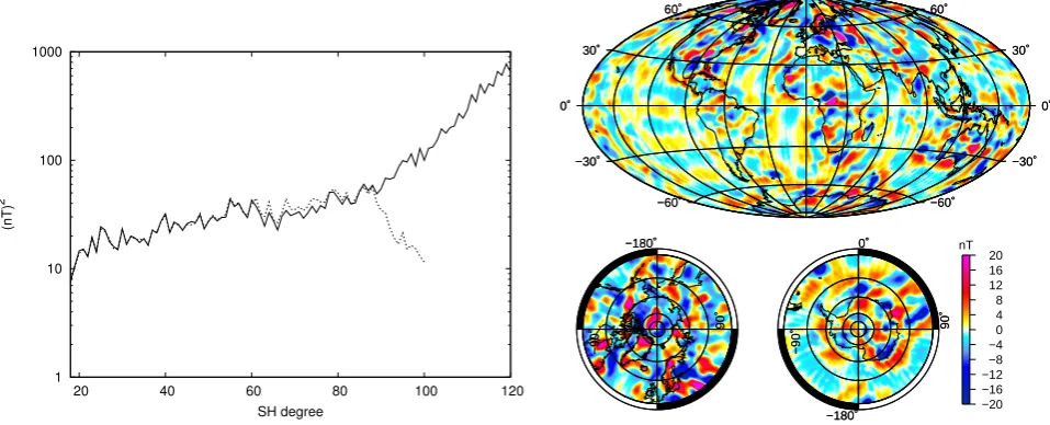
Kursk anomaly in western Russia, are clearly identifiable on this residual map, although they are not associated with too large residuals. There are very large clusters of residuals at high latitudes, and some of these residuals obviously corre-spond to lithospheric magnetic anomalies – e.g. North Amer-ica, southern tip of Greenland, Northern Europe. This is an incentive to work with a localized system of representation and to define local constraints. Here, we want to keep the processing as simple as possible and did not follow such ap-proaches. It should be noted, however, that the amplitude of the residuals are clearly smaller than 1.5 nT and that there is only few traces of the “along-track” noise in these residuals. The effect of the smoothing on the model remains acceptable. Figure 6, right side, shows the power spectra of the field model Bi and of the noise model B˜i. Also plotted is the spectrum from MF7. The damping parameterλ in Eq. (17) has been adjusted toλ=4.0 10−5_{such that the power} spec-trum does not present excessively high values at high de-grees. Overall, the derived map has the same level of energy as MF7 up to degree 100. Above that degree the spectra is clearly decreasing. Our opinion is that we are reaching at these SH degrees the maximum “global” resolution of the CHAMP data selected and processed following the technique described above. Improvements are probably still possible lo-cally, particularly above the largest anomalies seen as Bangui and Kursk anomalies.

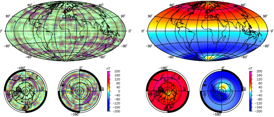
Figure 7, left side, maps the noise modelB˜i, and, on the right side, maps the perturbation model defined in Eq. (A1). The noise model presents the expected east–west high fre-quency oscillations. The map cannot be directly compared with Fig. 5 because the patterns of the oscillations in Fig. 7 correspond to the noise present in Bˆi; Fig. 5 is only a smoothed version of it. The perturbation model (Fig. 7, right side) is dominated by a dipole term consistent with un-modelled contributions generated in 1-D conductive layers of the Earth by a large-scale, rapidly varying external field. Although this large-scale field is dominant, higher spherical harmonic contributions exist in the perturbation model and are determinant for the success of the post-processing.

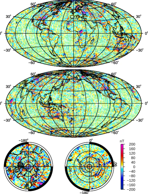
Our final result is a map of the vertical down component of the lithospheric field calculated at the Earth’s surface (see Fig. 8). The map includes all SH degrees of the lithospheric field model. The model is displayed with two different cen-tral meridians for a better view of the anomaly patterns. The anomaly patterns are not as clearly defined as in MF7, but in numerous areas – e.g. the northern Pacific – the result-ing map from our processresult-ing is remarkably detailed. How-ever, in the present case, the only difference with regards to a straightforward least-squares approach is the co-estimation of the noise model. In particular, there are no pre-processing steps such as data levelling (or micro-levelling) with mostly unknown consequences on the final map, and the only data used are the CHAMP satellite data. We have run numerous experiments, and it appears that the determinant step for the final quality of the map is the data selection used to build

−60˚ −60˚

−30˚ −30˚

0˚ 0˚

30˚ 30˚

60˚ 60˚

−60˚ −60˚

−30˚ −30˚

0˚ 0˚

30˚ 30˚

60˚ 60˚

−180˚

−90˚

0˚

90˚

−180˚

−90˚

0˚

90˚

−180˚

−90˚

0˚

90˚

−180˚

−90˚

0˚

90˚

−10 −8 −6 −4 −2 0 2 4 6 8 10 nT

1 10 100 1000

20 40 60 80 100 120 140

(nT)

2

SH degree

Fig. 6. Left: Residuals map to the final model fit to (noisy) lithospheric fieldBˆ_iatr=6671.2 km. Residuals have been scaled by a factor 10. At mid-latitudes the largest residuals are associated with the strong magnetic anomalies. The along-track noise has been fitted by the noise model and therefore does not appear in these residuals. Right: Power spectra of the lithospheric field modelB_i(solid line), of MF7 (dashed line), and the noise model (dotted line) calculated at the Earth’s surface (i.e.r=6371.2 km radius).

−60˚ −60˚

−30˚ −30˚

0˚ 0˚

30˚ 30˚

60˚ 60˚

−60˚ −60˚

−30˚ −30˚

0˚ 0˚

30˚ 30˚

60˚ 60˚

−180˚

−90˚

0˚

90˚

−180˚

−90˚

0˚

90˚

−180˚

−90˚

0˚

90˚

−180˚

−90˚

0˚

90˚

−200 −160 −120 −80 −40 0 40 80 120 160 200 nT

−60˚ −60˚

−30˚ −30˚

0˚ 0˚

30˚ 30˚

60˚ 60˚

−60˚ −60˚

−30˚ −30˚

0˚ 0˚

30˚ 30˚

60˚ 60˚

−180˚

−90˚

0˚

90˚

−180˚

−90˚

0˚

90˚

−180˚

−90˚

0˚

90˚

−180˚

−90˚

0˚

90˚

−200 −160 −120 −80 −40 0 40 80 120 160 200 nT

Fig. 7. Left: Map of the vertical down components of (left) the noise model and (right) the perturbation model. Both maps have been

calculated atr=6371.2 km radius. By definition, the perturbation model is very smooth in longitude, but that does not preclude a large complexity for the noise model.

the modelBˆi. Out of all these trials, the maps presenting the lowest level of noise are systematically the outputs of step 2 of our iterative inversion process. We decided not to show these results here because they are not consistent with the noise model presented in Appendix A that assumes a model derived through a non-regularized scheme. It is, however, an approach worth studying. There are no major difficulties in estimating what the noise model should be for a lithospheric model built using a regularized least-squares process.

4 Conclusions

−60˚ −60˚

−30˚ −30˚

0˚ 0˚

30˚ 30˚

60˚ 60˚

−60˚ −60˚

−30˚ −30˚

0˚ 0˚

30˚ 30˚

60˚ 60˚

−60˚ −60˚

−30˚ −30˚

0˚ 0˚

30˚ 30˚

60˚ 60˚

−60˚ −60˚

−30˚ −30˚

0˚ 0˚

30˚ 30˚

60˚ 60˚

−180˚

−90˚

0˚

90˚

−180˚

−90˚

0˚

90˚

−180˚

−90˚

0˚

90˚

−180˚

−90˚

0˚

90˚

−200 −160 −120 −80 −40 0 40 80 120 160 200 nT

Fig. 8. Map of the vertical down components of the final

litho-spheric field modelB_i. The map has been calculated at the Earth’s surface (6371.2 km). Although some noise is still visible in the northern Atlantic and over the southern polar cap, the noise level over mid-latitudes has been greatly reduced. Anomalies are partic-ularly well defined over continents, and Indian and Pacific oceans.

vector gravimetry or gradiometry may be possible. We made several strong hypotheses to obtain these results. Particularly, we consider that the orbits are exactly polar, that they are at constant radius and that the sampling rate along an orbit is “ideal” – i.e. the relationhP_l|m|, P_l|0m|i ∝δll0 is verified. We

also make the assumption that the lithospheric field model is derived through a simple un-regularized least-squares pro-cess. This latter approximation is well verified for our appli-cation, but the three former are rather rough – e.g. in our data set the altitudes varies between 480 km and 250 km. How-ever, it appears that the final result does not suffer too much from these hypotheses. We insist here on the fact that the noise models do not represent the expected noise in the satel-lite data but the noise leaking into the derived lithospheric models.

It is interesting to note that the amplitude of the noise gen-erated depends on the variance of the random variableχ_mk, which itself depends on the variance of the external field scaling factorηand the number of orbitsM (see Table 1).

Therefore, the usual choice of rejecting a significant part of the data because of its level of noise is questionable. For ex-ample, when dealing with magnetic data, rejecting a full year of satellite data because of the high level of magnetic activity is unlikely to reduce the noise level in the model since the ratio v_Mη generally does not get smaller. We cannot comment, however, on a data rejection criteria based on the satellite al-titude.

Another remarkable property of the noise models is their weak dependence with regard to the source of the noise. We used here perturbation models either from internal or external origin, but both lead to similar noise models. The same devel-opments could be done for a noise described by spherical har-monics without reference to any specific source. For the case where only radial component data are used (Eqs. 11, 12), such a hypothesis would not make any difference.

In the application to real data, the noise models were es-timated in a post-processing scheme. The reason for this choice is that we did not know what kind of perturbation modelBp(θ, φ, r)should be used. We have seen that for de-riving a lithospheric field model, a dipole perturbation model is not leading to the best results. In an ideal case where the perturbation model is known, the best approach to the prob-lem would be to build a covariance matrixCn for the noise

from the variances given in Table 1 and Eq. (A12). Such a covariance matrix could then be used as a regularization ma-trix in the least-squares fit of the lithospheric field model to the satellite data. However, even if the information provided by the estimated variances has not been used in our post-processing scheme, the resulting lithospheric field model is nonetheless much improved compared to what can be ob-tained through a simple smoothing (see the differences be-tween Fig. 8 and Fig. 5).

One can question if parts of the lithospheric field can be removed by our post-processing steps and contribute to the noise model. The lithospheric noise model derived is only a combination of spherical harmonics with some strong corre-lations between the Gauss coefficients. Therefore, there is no doubt that part of the true lithospheric magnetic field model can contribute to the noise model. It is, however, not possi-ble to estimate a priori what this part is because it clearly de-pends on both the noisy lithospheric field model on which the post-processing is applied and on the true lithospheric field we want to estimate. In order to test our scheme, we have first applied the processing on a synthetic data set built on a Gauss–Legendre grid where both the lithospheric field model and the noise are known. We used only the radial compo-nent of the field and verified that the noisy lithospheric field model derived from these data was contaminated by a noise corresponding exactly to Eq. (12). However, the full inver-sion process revealed that part of the lithospheric field was seen as noise. We also applied step 2 of our processing using a noise-free synthetic lithospheric field model and the noise model defined by Eq. (A12). Here again, despite a noise-free data set, the lithospheric field is partly interpreted as noise.

The amplitude of the obtained noise model is relatively large where there are strong anomalies, more or less aligned along orbits. This is the case for the Kursk anomaly (51◦_{N, 37}◦_E),

whereas the Bangui anomaly (4◦N, 16◦E) is apparently not affected by the processing. Outside a few localized areas, the noise model remained relatively small. This impossibility to properly separate the noise from the lithospheric field is a common limitation of all existing processing methods. In our specific scheme, the only way we can reduce this effect is by constraining the perturbation model. We therefore recom-mend that the post-processing is used only when the noise is clearly identifiable at the smallest wavelengths, constrain-ing this way the perturbation model. Overall, the proposed post-processing probably performs better than other smooth-ing techniques but that should to be tested on a case-by-case basis.

The work presented here opens numerous possibilities for processing data acquired along linear paths, such as satel-lite data. The major difficulty when dealing with large data set is to handle the correlated errors. Facing this problem we have here simply calculated how this correlated noise affects the derived model through a least-squares process. Extend-ing this to regularized least-squares approaches is certainly possible. The same technique can be applied for calculating small-scale secular variations from satellite data, or to pro-cess yearly estimates of the core field. The technique is also applicable for airborne data using any local system of repre-sentation rather than spherical harmonics. Interesting devel-opments are possible through the design of local filters. The link with oriented wavelets on the sphere is also promising.

Appendix A

Noise model for three component vector data

We follow here the same developments as in Sect. 2 but con-sider the case where the perturbation field is of internal origin and the three magnetic vector components are used. The per-turbation field can be written

Bp(θ, φ, r)= −∇

"

a L

X

l,m (a

r) l+1_ım

l Ylm(θ, φ)

#

. (A1)

It is scaled at each orbit by a factorηand is fitted by least-squares with a field of internal origin constant in time. There-fore we minimize the functional:

8=X i,j

wi|B˜i(θi, φj, r)−ηj·Bp(θi, φj, r)|2, (A2)

where the noise modelB˜iis defined by

˜

Bi(θ, φ, r)= −∇

"

a L=120

X

l,m (a

r) l+1_g˜m

l Y m l (θ, φ)

#

. (A3)

This leads to a linear system equivalent to Eq. (5), where the left-hand side can be written:

{At_A}

l,m,l0_,m0=(a

r)l

+l0+4_(l+1)(l0₊₁₎ P

i,j{wiY_lm(θi, φj, r)Ym

0

l0 (θi, φj, r)} +(a_r)l+l

0₊₄

P

i,j{wi∇hY_lm(θi, φj, r)·∇hYm

0

l0 (θi, φj, r)}.

(A4)

The operator∇_his the horizontal gradient on a sphere of unit radius. The first term in the right-hand side does not present difficulties. For the second term we use the following iden-tity:

Y_lmY_lm00= |l+l0|

X

L=|l−l0_| X

M

CL,M_l,l0_,m,m0Y_LM. (A5)

Applying twice the gradient operator gives

∇_hY_lm·∇_hY_lm0 0=

l(l+1)+l0(l0+1)

2 Y

m l Y

m0

l0 (A6)

−1

2

|l+l0| X

L=|l−l0_| X

M

C_l,lL,M0_,m,m0L(L+1)Y_LM.

Equation (A4) then becomes

{At_A}

l,m,l0_,m0=(a

r)l

+l0+4(l+l0_+1)(l+l0₊₂₎

2

P

i,j{wiY_lm(θi, φj, r)Ym

0

l0 (θi, φj, r)} −(a_r)l+l

0₊₄ P|l+l0_|

L=|l−l0_| P

MC

L,M l,l0_,m,m0

L(L+1) 2

P

i,jwiY_LM(θi, φj, r).

(A7)

Defining5mm0as in Eq. (8) gives in the limit of a large

num-berMof orbits 5mm0'(

1 2+

1

2δm0)δmm0.

Further, the weightswi are chosen such that

X

i

wiPlm(cosθi) P_lm0 (cosθi)=

4−2δm0 2l+1 δll0, which reduces forl0=0 toP

iwiP_lm(cosθi)=2δm0δl0. As a consequence, for the second term in the right-hand side of Eq. (A7), only the termL=0 remains. It therefore vanishes because of the factorL(L+1)and we obtain

{AtA}_l,m,l0_,m0=2M (

a

r)

2l+4_{(l+1) δ}

ll0δ_mm0. (A8)

The matrix AtA is therefore diagonal: The discrete

summa-tions in Eq. (A4) are equivalent to continuous integrasumma-tions. The product{At _b}

l,m in the right-hand side of Eq. (5) now

can be written

{At b}_l,m=MPN

n,k(ar)l

+n+4

{(l+1)(n+1)P

i,jηjwiY_lm(θi, φj, r)Ynk(θi, φj, r)

+P

i,jηjwi∇hYlm(θi, φj, r)·∇hYm

0

l0 (θi, φj, r)}.

(A9)

We further introduce the variableχ˙_mk defined by

˙ χ_mk =

 



χ−−mk ifmk >0 −χ−−mk ifmk <0

0 ifmk=0,

where the expression of χ_mk is given in Eq. (10). Equa-tion (A9) becomes

{Atb}_l,m=MPN

n,k ınk(ar) l+n+4

{(l+1)(n+1)hPn|k|, P

|m|

l iχmk+ h∂θP

|k|

n , ∂θP

|m|

l iχmk

+ h|k|P

|k|

n sinθ ,

|m|P_l|m| sinθ i ˙χ

k m},

(A11)

leading, when combined with Eq. (A7), to

˜

gm_l =PN

n,k ınk(ar) n−l {n+1

2 hP

|k|

n , P

|m|

l iχmk+2l1+2h∂θP

|k|

n , ∂θP

|m|

l iχmk

+ 1

2l+2h

|k|Pn|k| sinθ ,

|m|P_l|m| sinθ i ˙χ

k m}.

(A12)

TheL(L+2)Gauss coefficientsg˜_lmof the noise model can be represented by onlyN (N+2)coefficientsı_nkof the pertur-bation model and(2N+1)(2L+1)−2N2independent ran-dom variablesχ_mk, where all symmetry properties have been accounted for.

Appendix B

Estimating the variance ofχ_mk

The random variableχ_mk has been defined above by

χ_mk =

 



1 M

PM

i=1cosmφi coskφi ηi ifm, k≥0 1

M

PM

i=1cosmφi sin|k|φi ηi ifmk <0 1

M

PM

i=1sin|m|φi sin|k|φi ηi ifm, k <0,

(B1)

where ηi is a random variable with zero mean and

nor-mally distributed with variancevη. Let us consider first the simplest case wherem, k≥0. If we introduce the two vec-tors D= [cosmφi coskφi]i=1,M and N= [ηi]i=1,M, then

Eq. (B1) can be written χ_mk = 1

M D

t_{.N. (B2)}

With this definition it is clear that vχ= 1

M2D t_.C

N.D, (B3)

wherevχ is the variance ofχ_mk and CN=vηId, with Id

be-ing the identity matrix. We therefore obtain

vχ= v η

M2 { M

X

i=1

(cosmφi coskφi)2}, (B4)

and using the identity cosacosb=1

2(cos(a−b)+cos(a+b)) it follows that

vχ= v η

4M2 M

X

i=1

{(cos(m+k)φi)2+(cos(m−k)φi)2 (B5) +2(cos(m+k)φi cos(m−k)φi)}.

Over the CHAMP mission there is a large number of orbits and theφi are uniformly distributed between[0;π].It

fol-lows that the last term on the right-hand side vanishes unless k=0 orm=k=0,and it can be verified that

M

X

i=1

(cosnφi)2= M

X

i=1

(sinnφi)2= M

2 (B6)

as long asnis not too large. Therefore comes the following results:

– ifk=m=0,vχ=vη M

– ifk=0 andm6=0,vχ= vη

2M

– ifm=k6=0,vχ=3vη

8M

– ifm, k6=0,m6=k,vχ= vη

4M

Extending these results to the two other cases (i.e.km <0 andm, k <0) is straightforward.

Acknowledgements. We would like to acknowledge the work of

CHAMP satellite data processing team. M. R. was supported through the DFG grant: LE 2477/3-1 in the framework of the SPP-1488 “Planetary magnetism”. IPGP contribution number: 3340.

Edited by: F. Speranza

References

Hamoudi, M., Quesnel, Y., Dyment, J., and Lesur, V.: Aeromagnetic and Marine Measurements, in: Geomagnetic Observations and Models, edited by: Mandea, M. and Korte, M., IAGA book se-ries, 5, 57–105, Springer, doi:10.1007/978-90-481-9858-0, 2010. Holme, R.: Modelling of attitude error in vector magnetic data: ap-plication to Ørsted data, Earth Planet. Space, 52, 1187–1197, 2000.

Holme, R. and Bloxham, J.: The treatment of attitude errors in satel-lite geomagnetic data, Phys. Earth Planet. In., 98, 221–233, 1996. Hulot, G., Olsen, N., and Sabaka, T. J.: The present field, Treatise in Geophysics, Geomagnetism, Elsevier Ltd., Amsterdam, 2007. Kahaner, D., Moler, C., and Nash, S.: Numerical Methods and

Soft-ware, Prentice-Hall, ISBN 978-0-13-627258-8, 1989.

Kusche, J.: Approximate decorrelation and non-isotropic smoothing of time-variable GRACE-type gravity field models, J. Geodesy, 81, 733–749, doi:10.1007/s00190-007-0143-3, 2007.

Langel, R. A., Estes, R. H., and Sabaka, T. J.: Uncertainty estimates in geomagnetic field modelling, J. Geophys. Res., 94, 12281– 12299, 1989.

Lesur, V., Wardinski, I., Rother, M., and Mandea, M.: GRIMM – The GFZ Reference Internal Magnetic Model based on vector satellite and observatory data, Geophys. J. Int., 173, doi:10.1111/j.1365-246X.2008.03724.x, 2008.

Lesur, V., Wardinski, I., Hamoudi, M., and Rother, M.: The second generation of the GFZ Reference Internal Magnetic field Model: GRIMM-2, Earth Planet. Space, 62, 765–773, doi:10.5047/eps.2010.07.007, 2010.

Lesur, V., Wardinski, I., Hamoudi, M., Rother, M., and Kunagu, P.: Third version of the GFZ Reference Internal Magnetic Model: GRIMM-3, in: IUGG2011, MR207, Melbourne, Australia, 2011. Lowes, F. J. and Olsen, N.: A more realistic estimate of the vari-ances and systematic errors in spherical harmonic geomagnetic field models, Geophys. J. Int., 157, 1027–1044, 2004.

Maus, S., Yin, F., L¨uhr, H., Manoj, C., Rother, M., Rauberg, J., Michaelis, I., Stolle, C., and M¨uller, R. D.: Resolution of di-rection of oceanic magnetic lineations by the sixth-generation lithospheric magnetic field model from CHAMP satellite mag-netic measurements, Geochem. Geophys. Geosyst., 9, 949, doi:10.1029/2008GC001, 2008.

Olsen, N., Glassmeier, K.-H., and Jia, X.: Separation of the Mag-netic Field into External and Internal Parts., Space Science Re-views, 152, 135–157, doi:10.1007/s11214-009-9563-0, 2010a.

Olsen, N., L¨uhr, H., T. Sabaka, T., Michaelis, I., Rauberg, J., and Tøffner-Clausen, L.: CHAOS-4 – A high-resolution geomagnetic field model derived from low-altitude CHAMP data, in: AGU Fall Meeting, Poster GP21A-0992, San Francisco, 2010b. Piessens, R., Doncker-Kapenga, E., ¨Uberhuber, C., and Kahaner,

D.: Quadpack, A Subroutine Package for Automatic Integra-tion, Springer Series in Computational Mathematics, 1, Spinger-Verlag, ISBN 978-3-540-12553-2, 1983.

Reigber, C., L¨uhr, H., Schwintzer, P., and Wickert, J., eds.: Earth Observation with CHAMP Results from three years in orbit, Springer-Verlag, 2005.

Rygaard-Hjalsted, C., Constable, C. G., and Parker, R. L.: The in-fluence of correlated crustal signals in modelling the main geo-magnetic field, Geophys. J. Int., 130, 717–726, 1997.

Th´ebault, E., Purucker, M., Whaler, K., Langlais, B., and Sabaka, T.: The Magnetic field of the Earth’s lithosphere, Space Sci. Rev., 155, 95–127, doi:10.1007/s11214-010-9667-6, 2010.