Construction of stratification points under optimum allocation using dynamic programming

(1)

dynamic programming

Faizan Danish

Division of Statistics and Computer Science Faculty of Basic Sciences

SKUAST-JAMMU,J&K,India-180009 [email protected]

Abstract

In the present investigation, some theory has been developed for optimum stratification, when two auxiliary variables treated as the basis of stratification with one study variable under study. The problem has been formulated as mathematical programming problem and then solved by dynamic programming. Empirical studied have been made to illustrate the proposed method with the comparisons of other existing methods.

Keywords: Optimum allocation; Multistage decision problem; Cost function Introduction

Let the target population consisting of ‘N’ units be stratified into LM strata based on two auxiliary variables ‘X’ and ‘Z’ when the estimation of mean of the study variable ‘Y’ is of interest. In order to have the estimate ,we divide the whole population into the desired number of strata like LM such that each strata is homogenous within itself and heterogeneous between strata with respect to the character under study such that the number of units in the (h, k)th_{stratum is N}

hk ,such that

1 1

L M hk

h k

N N

= = =



From each of the stratum, a sample of size nhk is to drawn such that a total of ‘n’ units of

sample would be selected from a population consisting of size ‘N’. Let the sample size selected from (h , k )th stratum be ‘nhk’ ,such that

hk

h k

n =n



Let y_hki ,( i=1,2,3,...,Nhk) denotes the population unit in the (h ,k )th stratum ,then the

population total can be expressed as

hki

h k i

y=



y

Under stratified random sampling the unbiased estimator of the population meanY_N ,is

hk

st hk

h k

y =



W y

where , 1

hki hk

hk i

y y

n

=



and ‘Whk’ denotes the weight of the (h, k)th stratum as given as

hk hk

N W

(2)

The basic consideration involved in the determination of optimum strata boundaries (OSB) is that the strata should be internally as homogenous as possible, that is, the stratum variances should be as small as possible, given some sample allocation. When it is difficult to made stratification on the basis of study variable we make use of information highly related with the stud variable known as auxiliary information. The determination of OSB was pioneered by Dalenius (1950). Moreover several other authors have developed methods using study variable as stratification variable as well as auxiliary variable used as stratification variable. Dalenius and Gurney (1951) developed a technique with respect to an auxiliary variable closely related to study variable. Singh and Sukhatme (1969) considered the problem of finding approximately optimum strata boundaries on an auxiliary variable for one estimation variable. Further several authors have developed several methods at different allocation procedures like Singh, R. (1975), S.E.H. Rizvi et al. (2002) , Khan et al. (2003),Gupta et al. (2005),Rao et al. (2012),Khan et al. (2015).Danish and Rizvi (2017a) discussed made an attempt to cover all the developed methods made towards construction of strata boundaries. Danish et al .(2017) developed a method of obtaining optimum strata boundaries when the cost of every unit varies in the whole strata. Further development on optimum strata boundaries has been made by Danish and Rizvi (2018), Danish, F. (2018) and Danish and Rizvi (2019).

In this paper, the author is going to develop a method under optimum allocation using two stratification variables and one study variable.

Formulation of Problem under Optimum allocation

In stratified sampling, variance of the estimator depends on values of n_hk (h=1,2,...,L ;1,2,3,...,M) apart from values of Y. Even for a fixed n, the values of the

( )

st

V y will differ for different configurations

(

n=n₁₁,...,n_LM

)

.The combination ‘n’ for which V y

( )

_st is minimum among all the values of variances for different possible combinations ‘n’ is an optimal allocation for a fixed n. Since sampling involves cost in a survey, consider the linear cost function

0 hk hk

h k

C=C +



C n (1)

where C0 is an overhead cost (e.g cost of setting up and maintaining an office ,recruiting

survey personal and other capital expanses etc.) Chk is the cost of sampling unit from the

(h,k)th stratum and C is the total cost.(1) equation is a very simple and reasonable cost function expressing the total cost of field operation. The variance under stratified random sampling is

( )

hk2 hky2 hk hky2 st

hk hk

h k h k

W W

V y

n N

 

=



−



(2)

To determine the value of n_hk , consider the function

( )

st

V y C

 = + (3)

(3)

Using the calculus method of Langrangian multiplier, select n_hkand a constant to minimize  .

Differentiating (3) w.r.to n_hk,we have 2 2

2

, 1, 2,..., 0

1, 2,...,

hk hky

hk hk

W h L

c

K M

n



 =

− + =

=

hk hky hk

hk

W n

c  

 = (4)

while taking summation on both sides ,we get

hk hky

h k hk

W n

c

 

 

= _ _

 



(5)

From (4) and (5),we can obtain

hk hky hk hk

hk hky hk

h k

W

c

n n

W

c 

 =

 

 

 



(6)

Thus (6) relation leads to the following important conclusion that, in a given strata, we have to take a large sample size if

i. the stratum size is large.

ii. the stratum has large variability.

iii. the cost per unit is cheaper in the stratum.

The sample size ‘n_hk’ from

( )

h k, th stratum required for estimating the population with a specified cost ‘C’ is given by

(

0

)

hk hky

hk hk

hk hky hk

h k

W

C c

c n

W

c 

 −

=

 

 

 



(7)

If c_hk's are the same from stratum to stratum, relation (7) will lead to Neyman allocation. Similarly if c_hk's and _hky's doesn’t vary from stratum to stratum, relation (6) leads to proportional allocation.

Now, substituting (7) in (2),we get

( )

(

)

2

0 hk hky hk

hk hky h k

st

h k hk

W c

W V y

C c N

 _

 

 

 

= −

−



(8)

(4)

( )

st hk hky hk

h k

V y =



W  c

(9)

When the study variable ‘Y’ itself is not used for stratification variable, we propose a model based on bi-variate stratified sampling design. Let the regression model of study variable on auxiliary variables is of the form as

( )

,

Y = x z + (10)

where,

( )

x z, be a linear function of ‘X’ and ‘Z’ and is equal to  + x+z and ‘



’ denotes the error term such that

(

)

0

( , )

E

x z

 ₌ _and

(

)

( )

_,

( , )

V x z

x z

 ₌_ _{for all (x,z)}

Under model (10) the stratum mean ‘_hky’ and the stratum variance ‘_hky2 ’ can be written as

hky hk

 = (11)

and

2 2

hky hk hk

 = + (12)

where _hk_and _hk_are the expected value of 

( )

x z, and 

( )

x z, respectively and _hk2 _ denotes the variance of ( , )x z in the (h,k)th_stratum.

If ‘ ‘and ‘



‘are uncorrelated, then ‘_hky2 ’ can be expressed as

2 2 2

hky hk hk

 = + (13)

where _hk2_ is the variance of in (h, k)th_{stratum. It can be verified by (12) and (13) .}

If the joint density function of (X,Y,Z) in the super population is f(x, y, z) and joint marginal density function of X and Z is f(x, z) .Let f(x) and f(z) be the frequency function of the auxiliary variables X and Z respectively defined in the interval [a, b] and [c, d].

If the population mean of the study variable ‘Y’ is estimated under the variance given in equation (2.9) ,then the problem of determining the strata boundaries is to cut up the ranges V=b-a and U = d-c, at (L-1) and (M-1) intermediate points as

0 1 ... L 1 L

a=x   x x ₋ x =b and

0 1 ... M 1 M

c=z   z z ₋ z =d respectively such that the equation (9) is minimum.

If f x z

( ) ( )

, , x z, and 

( )

x z, are known and also imtegrable then, W_hk,_hk2_ and _hk_can be obtained as a function of boundary points

(

x x_h, _h₋₁,z z_k, _k₋₁

)

by using the following expression

( )

1 1

,

h k

x z

hk _x _z

W f x z x z

− −

=

 

  (14)

( ) ( )

1 1

2 1 2 2

, ,

h k

x z

hk _x _z hk

hk

x z f x z x z W

 

  

− −

(5)

and

( ) ( )

1 1

1

, ,

h k

x z

hk _x _z

hk

x z f x z x z W



 

− −

=

 

  (16)

Where,

( ) ( )

1 1

1

, ,

h k

x z

hk _x _z

hk

x z f x z x z W



 

− −

=

 

 

(17) where

(

x_h−x_h₋₁

)

and

(

z_k −z_k₋₁

)

are the boundary points of the (h,k)th stratum. If a simple random sample of size ‘nhk’ drawn from (h, k)th stratum unbiased estimator of

x and y can be obtained as

st _hk hk

h k

x =



W x , _st _hk _hk

h k

y =



W y

where xst and y_hk are the unbiased sample estimator of XhkandYhk.

However for ‘X’ and ‘Z’ independent of error term ‘ε’ then

2 2 2 2 2

hky hkx hkz

 =  +  (18) Thus the variance that we need to minimize is

( )

(

2 2 2 2

)

hk hkx hkz hk

st

h k

V y =



W   +  c

the weight and variance of the (h,k)th stratum having auxiliary variables as ‘X’ and ‘Z’.

( )

1 1

,

h k

x z

hk _x _z

W f x z x z

− −

=

 

  (19)

( )

1 1

2 1 h 2 k 2

h k

x z

hkx _x _z hkx

hk

x f x x z

W

 

− −

=







 − (20)

( )

1 1

2 1 k 2 h 2

k h

z x

hkz _z _x hkz

hk

z f z z x

W

 

− −

=







 −

(21)

where

( )

1 1

1 h k

h k

x z

hkx _x _z

hk

x f x x z

W



− −

=







 ,

( )

1 1

1 k h

k h

z x

hkz _z _x

hk

z f z z x

W



− −

=









Thus the objective function (1) could be expressed as the function of boundary points

(

x xh, h−1,z zk, k−1

)

only.

Let 

(

x x_h, _h₋₁,z z_k, _k₋₁

)

=W_hk_hky c_hk (22) we have already let the range

0

x L

d = − =b a x −x (23)

0

z M

t = − =d c z −z (24)

Then, in the bivariate stratification a problem of determining the strata boundaries

(

x zh, k

)

is to break up the ranges of (23) and (24) at intermediate points in order to estimate 1x x2...xL−2xL−1 and

1 2 ... M 2 M 1

z z _ z ₋ z ₋ .Then, the reasonable criterion for determining optimum strata boundaries(OSB)

(

x z_h, _k

)

is to minimize

Minimize _hk

(

_h, _h ₁, _k, _k ₁

)

h k

x x z z

 ₋ ₋



(6)

0 1 ... L 1 L

a=x   x x ₋ x =b

0 1 ... M 1 M

c=z   z z ₋ z =d and

hk

h k

n =n



When, the marginal frequency function are known and _hky2 can be expressed as a function of boundary points

(

x z_h, _k

)

.For the rectangular stratification let V_h =x_h−x_h₋₁ and U_k =z_k −z_k₋₁ denotes the total length and width of the (h, k)th_{stratum. Then, using (23) and (24) ,the ranges can be expressed as}

(

1

)

h h h x

h h

V = x −x ₋ = − =b a d



(26)

(

1

)

k k k z

k k

U = z −z ₋ = − =d c t



(27)

Let *

(

1

)

1,

h

i x xh z

 −

− be the optimal value for the objective function (25) for the strata (h, k) to (L, k) for all k=1,2,...,M given that the lower bound for the strata (h,k) for k = 1,2,...,M is x_h₋₁.The functional equation of Bellman with respect to the first part of the ith iteration is then given by

(

)

₍ ₎

(

)

1

(

)

1

* 1

* 1 1 1

1 1 1

1 1

,

, , , , h

h

h h h

i M

x h

i i i

x h h h k k

V B x _k h h h

x z

x z Minimize x x z z

x x V



  +

−

− − −

− _ − − ₋

=

 

 

= _ + ₌ ₊ _

 







Using this last equation, new points of stratification xi with respect to the variable ‘X’ can be obtained to response the proceeding value i 1

x− .Hence the OSB for the first part of the ith iteration are given by

(

x zi, i−1

)

.For the second part of the ith iteration ,the points of stratification xi are in turn considered as fixed. Restating the problem of determining OSB as the problem of determining optimum points

(

V U_h, _k

)

,adding equation (26) and (27) as a constraint ,the problem (25) can be treated as an equation problem of determining Optimum Strata Width (OSW) ,

1, 2,..., L 1, 2,..., M

V V V and U U U and is expressed as the following MPP:

Minimize _hk

(

_h, _h ₁, _k, _k ₁

)

h k

x x z z

 ₋ ₋



Subject to (28)

h x

h

V =d



k z

k

U =t



,h=1,2,...,L and k =1,2,...,M

and

0 0

h k

V  andU 

(7)

will be the function of

(

V U₂, ₂

)

alone and so on. Due to special nature of function the MPP (28) may be treated as the function of

(

V U_h, _k

)

and can be expressed as:

Minimize _hk

(

_h, _k

)

h k

V U





Subject to (29)

h x

h

V =d



k z

k

U =t



,h=1,2,...,L and k =1,2,...,M

and

0 0

h k

V  and U 

The solution Procedure

The problem (29) is a problem of multistage decision in which the objective function and the constraints are separable functions of

(

V U_h, _k

)

, which allows us to use a dynamic programming technique. Dynamic programming determines optimal solution of a multi-variable problem by decomposing into stages, each stage compromising a single multi-variable sub problem. A dynamic programming model is generally a recursive equation. These recursive equations link te different stages of the problem.

Consider the following sub problem of equation (29) for first

(

L₁M₁

)

strata, where

(

L₁M₁

) (

 L M

)

,i,eL₁L M, ₁M

Minimize

(

)

1 1

, , ,

L M

hk h h k k

h k

x x z z

 ₋ ₋

= =



Subject to (30)

1

1 1

L

h L

h

V d

−

= =



1

1 1

M

k M

k

U t

−

= =



,h=1,2,...,L1 and k =1,2,...,M1

and

0 0

h k

V  and U 

where

1 , 1

L M

d V t M Note that if

1

L

d =V and

1

M

(8)

1 1

1 1 1 1

1 2

1 1 2 1

2 1 2 2 1 1

2 1 2 3 3

1 1 2 2

...

.

L L

L L L L

d V V V

d V V V d V

d V V d V

d V d V

− −

− − − −

= + + +

= + + + = −

= + = −

= = −

Similarly, we have

1 1

1 1 1 1

1 2

1 1 2 1

2 1 2 2 1 1

2 1 2 3 3

1 1 2 2

...

.

M M

M M M M

t U U U

t U U U t U

t U U t U

t U t U

− −

− − − −

= + + +

= + + + = −

= + = −

= = −

Let

(

)

(

)

1 1

1 1 1 1 1 1

1 1

,

L M

hk h k h k

L M L M L M

h L k M

h k

V U

V U Min

V d U t



 = =



= =

 

 

 = _ _

= =

 

 





1 1

0, 0; 1, 2,3,..., 1, 2,3,...,

1 , 1

h k

and V U h L and k M

and L L M M

  = =

   

Let

(

)

1 1 1, 1

L M dL tM

 _ denotes the minimum value of the objective function of the equation (30), that is,

(

)

(

)

1 1

1 1 1 1 1 1

1 1

1 1 1 1

1 1

, ,

,

L M

hk h k

h k

L M L M L M

h L k M

h k

V U

d t Min

V d U t

 

− −

= =

 − −

= =

 

 

=

 

= =

 

 

 



1 1

0, 0; 1, 2,3,..., 1, 2,3,...,

h k

and V  U  h= L and k = M

with the above definition of

(

)

1 1 1, 1

L M VL UM

 _ ,the MPP (22) is equivalent to finding

(

,

)

L M d tx z

 _ recursively by defining

(

)

1 1 1, 1

L M VL UM

 _ for

1 1, 2,..., 1 1, 2,...,

L = L and M = M ;

1 1

(9)

(

)

(

)

(

)

1 1 1 1

1 1

1 1 1 1

1 1

1 1 1 1

1 1 1 1 1 1 1 1 , , , ,

L M L M

L M

hk h k

L M L M

h k

L M

h L L k M M

h k

V U

V U

d t Min

V d V U t U

    − −  = = − − = =      _ _  _ _ = _ _   +  _ _   = − = −   _ _  

 



1 1

0, 0; 1, 2,3,..., 1, 2,3,...,

h k

and V  U  h= L and k = M

For fixed value of

(

)

1, 1 ,

L M

V U

1 1

0d_L V , 0t_M U.

(

)

(

)

(

)

1 1 1 1 1 1 1 1

1 1

1 1 1 1

1 1 1 1 1 1 1 1 , , , ,

L M L M L M L M

L M

hk h k

h k

L M

h L L k M M

h k

d t V U

V U Min

V d V U t U

     − − = = − − = = =       + _ _ = − = −      

 



and 1 1

0 , 1, 2,...,

0 , 1, 2,..., 1

h

k

V h L

U k M

 =

 = −

and

1 1

1 L L ,1M M

Using the same procedure to write the forward recursive equation of the dynamic programming technique and could obtain OSB.

Empirical Studies

I: If the variable is having right triangular distribution with pdf as

( )

2 2

(

)

; 0 1

0 ; x x f x otherwise  −    =   (31)

and the other variable follows an exponential distribution as

( )

; 0, 0

0 ; z e z f z otherwise   −     =   (32)

In order to obtain OSB when the auxiliary variables have as given above we need to estimate the values of W_hk,_hkx2 and _hky2 .For estimating this use above pdf’s in (19)-(21),we get

1

hk h

W =V g (33)

(

)

(

)

(

)

(

)

2

2 2 2 2 2

1 1 1 1 1 1

1 1 2 2 1 1 1 4 1 3

3 3 2 2 2 4

3 2

2 3

h h

k h h h h h h h h h h k

h h h

hkx

V V

U g V x V x V x V x V x U

x x V

(10)

(

)

(

)

(

)

(

)

(

)

(

)

(

)

(

)

2 2 2 ₁

1 1 1 1

2

2 ₂

1 ₁

1 1

2 2 1

1 4 2 ₁ ₄ ₂

k k

k k k

k _k

U U

U U U _k _k

k k k k k k

hkz _U

U

h h _h _h

z e U e

z U z e z U z e e

e V x _e _V _x

      _  _  − − − − − − − − − − − ₋ − ₋  ₊  ₋ ₋        − + + _ + + _+ − __ _ _ = − − − − ₋ _{− −} (35) where

(

)

(

)

1

1 1 4 2 1

k k

z U

h h

g e− − e− V x

−

= − − −

Using values obtained in equations (33)-(35) in MPP (29),we have Minimize

(

)

(

)

(

)

(

)

(

)

(

)

(

)

(

)

(

)

2 2 2 1 1 2 1 2 2

1 1 1 1 1

2 2 1 2 2 1 1 1 1 1 2 1 4 ₁

3 3 ₁

3 ₄ ₃

1

2 2 2 2 3

2

2 2 1

1 4 2

k

k k

k

h h h h

h h

k k

h h h h h h h h h

U h

k k k

U U

k k k

U

h h

V x V x _V _V

U g U

V x V x V x x x V

g

V g

z U z e

z U z e e

e V x

       − − − − − − − − − − − − − − − −  ₊ ₊  _ _ _ _   _ − _  ₋  _ _    _ _   ₋ ₊ ₊ ₊  _₊ ₋ ₋ _          ₋ ₊    + _ + + _+ − + − − − 

(

)

(

)

(

)

2 1 2 ₂ 1 1 1

1 4 2

k k k hk h k U U k k U h h c

z e U e

e V x

    − − − − −                _   _{ }      _ _{ }_ ₊ _ ₋ ₋ _   _ _{ −}__ _ _   _ _   _ _ ₋ _{− −}   _ _   _ _   



Subject to h x h k z k V d U t = =



(36)

1, 2,...,

0, 0 ,

1, 2,..., h k h L V U k M =    =

By executing a programme in R-software relating to generating random numbers for estimating the parameters we get β=1.52 and γ=0.42.

Now let us assume that the auxiliary variable X is defined in x

 

0,1 and Z in z

 

0, 6 i,e.

0 0, L 1, 0 0, M 6

x = x = z = z = and  = 1.we can write MPP (36) as

Minimize ( )

(

)

( )

(

)

( ) ( ) ( )

(

)

₍ ( ₎)

(

)

( ) 2

2 2 2 2 2

1 1 1 1 1 1

1 1 2 1 ₁ 2 2 1

1 1 1 1

1

1 1

4 1 ₃

' 3 3 2 2 2 4

3 2

2 3

2.31 '

1 1

2 2 1

0.17

1 4 2

k k k

k

h h

k h h h h h h h h h h k

h h h

h

U U U

k

k k k k k k

U

h h

V V U g V x V x V x V x V x U

x x V

V g _g

z e z U z e z U z e e

e V x

− − − − − − − − − − − − − − − − −   ₋      ₊ ₊ ₋ _ ₊ ₊ ₊ _₋  _ _   _ _ _ _   _₊ ₋ ₋ _   + −   − + + _ + + _+ − + − − − −

(

)

(

)

( ) 2 2 2 1

1 4 2

k k k hk h k U U k U h h c U e

e V x

(11)

1

6

h h

k k

V

U =

=



(37)

1, 2,...,

0, 0 ,

1, 2,...,

h k

h L

V U

k M

=

  

=

Where 1

(

)

(

)

1' 1 4 2 1

k k

z U

h h

g e− − e− V x

−

= − − −

while executing a computer programme of the MPP (37) for obtaining OSB of 6 (2×3) strata assuming the cost values asc₁₁=2,c₁₂ =3,c₁₃ =4,c₂₁=5,c₂₂ =6,c₂₃=7 ,we get Table 1: Displays the OSB when the auxiliary variables X and Z have pdf’s as right

triangular and exponential respectively

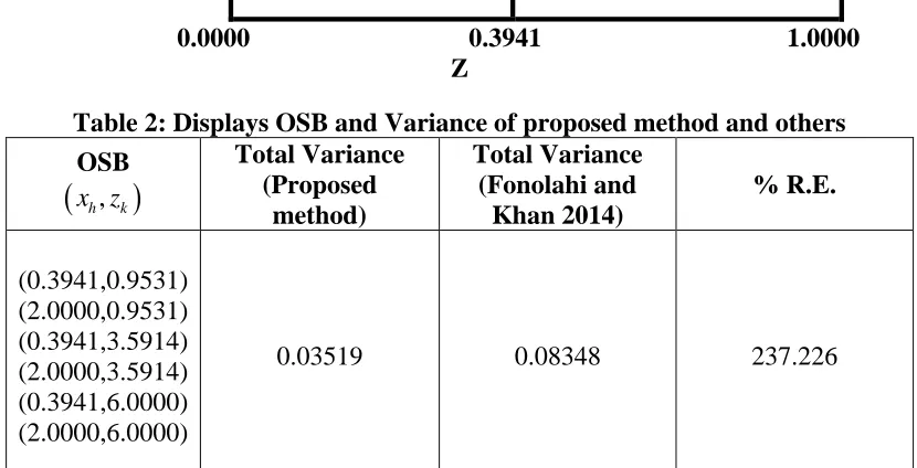
Table 2: Displays OSB and Variance of proposed method and others OSB

(

x z _h, _k

)

Total Variance (Proposed

method)

Total Variance (Fonolahi and

Khan 2014)

% R.E.

(0.3941,0.9531) (2.0000,0.9531) (0.3941,3.5914) (2.0000,3.5914) (0.3941,6.0000) (2.0000,6.0000)

0.03519 0.08348 237.226

Table 1 shows the stratification points when the auxiliary variables are having right triangular and exponential distribution. In order to obtain 6 strata in total from which two along the x-axis and 3 along the z-axis, the OSB obtained in case of optimum allocation are presented in Table 2 along with the variance obtained by using proposed method as well variance obtained by Fonolahi and Khan (2014).Thus it reveals that the variance obtained through the proposed method is lesser than the method proposed by Fonolahi and Khan (2014).The percentage of relative efficiency comes out to be 237.226. Hence the proposed method is preferable than the existing method.

II:Let us assume that the auxiliary variable X is having a uniform distribution with pdf as X

6.0000 3.5914 0.9531

(12)

( )

1 , ,

a x b

f x b a

o otherwise

 _{ }

 = −

 (38)

and assumed that the other variable Z is following standard normal distribution with pdf as

( )

2

2 1

; 2

0 ;

z

e z

f z

otherwise



− 

 _{−    }

=   

(39)

To obtain OSB for the study variable which is having two auxiliary variables following uniform and standard normal distributions, we need to find the values of W_hk,_hkx2 and

2 hky

 .For estimating this use above pdf’s in (19)-(21),we get

(

) ( )

1

2

h hk

V

W E

b a =

− (40)

(

)

(

)

( )

2

2 2 2

1 1 1 1

2

2 1

2 3 3 12 2

3

k h h h h k h h

hkx

U E V x V x U V x

E

 + − + − − + −

= (41)

(

)

(

)( )

(

)

( )

2

1 1

1 1 2

2 2

1 2

1 1

exp

2 2

exp

2 2

k k k

hkz

k k

k k k

z U z

z erf U z E

b a E

z z

z erf U z

 

− −

 ₋   + ₋ ₊ 

     

 

 

= − _ _+

   

₋ _₋ _ _ _₊ ₊ 

 _ _ _ _ 

 

(42)

where

1 1

1

2 2

k k k

U z z

E =erf _ + − _−erf _ − _

   

(

)

2

1 1

2 exp

2 2

k k k k

U z U z

E − erf −

 ₊  _ ₊ _

 

= − _ _

  _ _

 

,

(

)

2

1 1

3 exp

2 2

k k k

U z z

E − erf −

 ₊  _ _

 

= − _ _

  _ _

 

and ‘erf ’ is known as the error function and is given by

2

1

2

( ) ( ) k

k

z u

k k _z

erf z erf z e u

 −

− −

 

− =_ _ 

 



using values obtained in (40)- (42) in equation (36),we have

(13)

(

) ( )

(

)

(

)

( )

(

)

(

)

(

)

( )

2

2 2 2

1 1 1 1

2

2 1

2

1 1

1 1 2

2 2 1

2

1 1

1 1 3

2 1

2 3 3 12 2

3 exp 2 2 2 2 2 exp 2 2

k h h h h k h h

k k k

h

hkz

k k

k k k

E

z U z

z erf U z E

V

E b a

b a _z _z

z erf U z E

E     − − − − − − − − − − −  ₊ ₊ ₋ ₊      _ _ _ _ ₊ _ _  _ _₋ _ _ _₋ ₊ _    _ _ _ _ ₊ ₌ ₋      − _ _   _ _ _ − −  _ _+ +   _ _ _ _        +    hk h k c             



Subject to h x h k z k V d U t = =



(43)

1, 2,...,

0, 0 ,

1, 2,..., h k h L V U k M =    =

Let us assume that the interval of X is defined as x

 

0,1 and the variable Z be truncated at 4 i,ez

 

0, 4 and by simulation in R-software estimates β=1.07 and γ=0.73.Thus ,we have (43) as

Minimize

( )

(

)

(

)

(

)

( )

(

)

(

)

( )

2

2 2 2

1 1 1 1

2 1 2

1 1

1 1 2

1

2

1 1

1 1 3

2 1

3 3 6 2

2.28 3 exp 2 2 1.5 2 exp 2 2

k h h h h k h h

k k k

h

k k

k k k

E

z U z

z erf U z E

V E

z z

z erf U z E

E  − − − − − − − − − − −  ₊ ₊ ₋ ₊         _ _ _ _ ₊ _ _  _ _₋ _ _ _₋ ₊ _    _ _ _ _ ₊          ₋ _₋ _  ₊ ₊      _ _ _ _          +      hk h k c  



Subject to 1 4 h h k k V U = =



(44)

1, 2,...,

0, 0 ,

1, 2,..., h k h L V U k M =    =

For obtaining OSB we assume that the values of

11 2, 12 3, 13 4, 21 5, 22 6, 23 7

(14)

for total 6 (2×3) strata, execute a computer programme in LINGO by assuming all these conditions given above we have

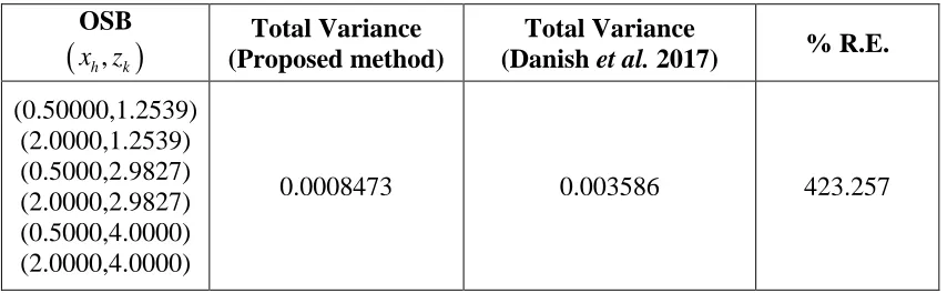
Table 3: Displays OSB and Variance of proposed method and others when having uniform and standard normal distribution

OSB

(

x z _h, _k

)

Total Variance (Proposed method)

Total Variance

(Danish et al. 2017) % R.E. (0.50000,1.2539)

(2.0000,1.2539) (0.5000,2.9827) (2.0000,2.9827) (0.5000,4.0000) (2.0000,4.0000)

0.0008473 0.003586 423.257

Table 3 presents the OSB and variances when the auxiliary variables X and Z follow uniform and standard normal distributions respectively. The percentage of relative efficiency between proposed method and Danish et al. (2017) method comes out to be 423.257.Thus it reveals that the variance obtained through the proposed method is lesser than the method proposed by Danish et al.(2017) .Hence the proposed method is preferable than the existing method.

Conclusion

In this investigation I have developed a method for construction of optimum strata boundaries under optimum allocation when we are having single study variable consists of two auxiliary variables. The problem happens to be multistage problem which was solved by dynamic programming by executing the programme in LINGO. It is found that the construction of strata using auxiliary variable of the populations having above mentioned distribution functions, leads to substantial gains in the precision of the estimates while using the proposed technique. Empirical studies showed that the proposed method is more precise than the methods developed by Fanolahi and Khan (2014) and Danish et al. (2017) that concludes the proposed method more preferable.

Acknowledgment

I am highly thankful to the reviewers for suggesting comments that improves the

quality of the paper. Further, the incredible efforts made by the Journal team especially Dr.Rehan Ahmad Khan and Kanwal Saleem towards the paper, deserves to be

acknowledged.

References

1. Dalenius, T. (1950). The problem of optimum stratification-II. Skand. Aktuartidskr, 33, 203-213.

(15)

3. Danish, F., Rizvi, S.E.H. Jeelani, Sharma, M.K. and M. I.J (2017). Optimum Stratification Using Mathematical Programming Approach: A Review. Stat. Appl. Pro. Lett. 4(3), 123-129

4. Danish, F., Rizvi, S.E.H. Jeelani, M. I and Reashi J.A. (2017).Obtaining Strata Boundaries under Proportional Allocation with Varying Cost of Every Unit. Pak.j.stat.oper.res. 13 (3): 567-574

5. Danish, F. and Rizvi, S.E.H. (2018): Optimum Stratification in Bivariate Auxiliary Variables under Neyman Allocation. Journal of Modern Applied Statistical Methods. 17(1).2580. DOI: 10.22237/jmasm/1529418671.

6. Danish, F. (2018): A Mathematical Programming approach for obtaining optimum strata boundaries using two auxiliary variables under proportional allocation. Transition in Statistics. 19(3).507–526, DOI 10.21307/stattrans-2018-028.

7. Danish, F. and Rizvi, S.E.H. (2019): Optimum Stratification by two Stratifying Variables using Mathematical Programming. Pakistan Journal Of Statistics. 35(1),11-24.

8. Fanolahi, A.V. and Khan, M.G.M. (2014). Determing the optimum strata boundaries with constant cost factor. Conference: IEEE Asia Pacific World Congress on Computer Science and Engineering (APWC), At Plantation Island, Fiji.

9. Gupta, R. K., Singh, R. and Mahajan, P. K. (2005). Approximate optimum strata boundaries for ratio and regression estimators. Aligarh J. Statist., 25, 49-55. 10. Khan, M.G.M. , Khan, E.A. and Ahsan, M.J. 2003. An optimal multivariate

stratified sampling design using dynamic programming. Aust. N. Z. J. Stat. 45(1): 107–113.

11. Khan, M. G. M. , Rao, D., Ansari, A.H. and Ahsan, M.J. (2015).Determining optimum strata boundaries and sample sizes for skewed population with log-normal distribution. Communication in statistics -simulation and computation, 44:1364-1387.

12. Rao, D., Khan, M.G.M. and Khan, S. (2012).Mathematical programming on multivariate calibration estimation in stratified sampling. World academy of science, engineering and technology.6:12-27.

13. Rizvi, S. E. H., Gupta, J. P. and Bhargava, M. (2002). Optimum stratification based on auxiliary variable for compromise allocation. Metron, 28(1): 201-215. 14. Singh, R. (1971). Approximately optimum stratification on the auxiliary variable.

J. Amer. Statist. Assoc., 66, 829-833.

15. Singh, R. (1975). An alternate method of stratification on the auxiliary variable. Sankhya, 37: 100-108.