Detecting Diabetes Mellitus using Machine Learning Ensemble

(1)

International Journal of Computer Systems (ISSN: 2394-1065), Volume 03– Issue 12, December, 2016 Available at http://www.ijcsonline.com/

Detecting Diabetes Mellitus using Machine Learning Ensemble

Madeeh Nayer Algedawy Institute of Public Administration

Dammam, Saudi Arabia

Abstract

Machine learning proved to be an excellent tool to detect and predict different medical issues. This paper applies sixdifferent machine learning techniques: Linear Discriminant Analysis, Generalized Linear Model, Recursive Partitioning and Regression Trees, Support Vector Machines, K-Nearest Neighbors and Naïve Bayes to Pima Indians Diabetes Database. The six developed models predict whether the patient is expected to suffer from diabetes or not. After comparing the performance of these algorithms through accuracy, precision, recall and f-measure. A stacking ensemble is built using them, and the final ensemble result proved to yield better results. Experimentations show that the stacking ensemble yields an accuracy of 94.27%, and f-measure of 0.956. This ensemble was stacked of LDA, KNN, and recursive trees; building a stacking ensemble on all the models yields much worse results due to high correlations. The best individual model is LDA which yields an accuracy of 77.6% and f-measure equals to 0.837.

Keywords: Diabetes; Ensemble; Stacking;LDA; GLM; SVM; NV; KNN; Recursive Trees; R..

I. INTRODUCTION

Diabetes mellitus is a chronic metabolic disease. In 2015, there were 415 million persons suffering from diabetes [1], with similar rates in males and females [2]. Its symptoms include high blood sugar, frequent urination and increased hunger and thirst [3]. Its complications include heart desease, kidney failure, eyes damage, coma and death [4]. Its two main reasons are either insulin is not sufficiently produced by pancreas or body cells are not responding to the produced insulin, therefore glucose will not be absorbed by the body cells and it will not be stored in the liver and muscles resulting in high blood sugar [5][6]. The three main types of diabetes are Type 1 DM, Type 2 DM and Gestational diabetes (pregnancy). It is always recommended to undergo a healthy diet, exercise regularly and avoid smoking [1].

In this paper, six machine learning algorithms are used to detect whether the person suffers from diabetes or not: Linear Discriminant Analysis, Support Vector Machine and Naïve Bayes. K-nearest Neighbors, Recursive Trees and Generalized Linear model, then a stacking ensemble is built aiming at achieving a better accuracy and f-measure by combining the models predictive powers. LDA depends on using dimension reduction techniques to maximize the difference among the classes. KNN is a simple non parametric classification algorithm, Recursive Trees is a classical decision trees that implements altered priors to judge different attributes. SVM is a very solid classifier frequently reported as the best classifier possible if fine tuning of its parameters is wisely handled and Naïve Bayes is a simple classifier that assume that predictors are independent. These six algorithms will be compared using a GLM wholistic classifier, and performance will be measured by generating the confusion matrix and calculating the accuracy, precision, recall and f-measure.

The Pima Indians Diabetes Database consists of eight predictors and one dependent variable, which indicate either the patient, has diabetes or not. The predictors mainly measure the ratio of sugar in blood, the patient body mass index and number of pregnancies taking into account the disease history. The six machine learning algorithms will focus on diagnosing diabetes. All the experimentations are implemented in R, which is a language and environment for statistical computing and graphics, it has a huge collection of machine learning and data mining algorithms and it is a little faster than WEKA and new packages are coming up very regularly.

This paper is organized as follows, section 2 provides the brief of the related work to applying machine learning to Diabetes Mellitus, section 3 gives a brief summary of the six classifiers used, section 4 declares the ensemble procedure followed to build the stacking model, section 5 provides a detailed description of the database and some important data explorations, section 6 represents the experimentations and comments on the results. Finally, section 7 concludes the result.

(2)

preprocessing techniques on the dataset.[12] implemented SVM on Pima Indians dataset and achieved an accuracy of 78%.[13] tested eight different algorithms: J48, KNN & ANFIS, GA, NB, PLS-LDA, Baysian, MLP and C4.5; J48 yielded the best accuracy equals to 99.87% where both MATLAB and WEKA were used.

III. CLASSIFIERS

Six classifiers are compared in this research: Linear Discriminant Analysis, Support Vector Machines, Naïve Bayes, Generalized Linear Model, K-Nearest Neighbors and Recursive Partitioning Trees.

3.1. Linear Discriminant Analysis

Linear Discriminant Analysis (LDA) focuses on maximizing the seperatibility among the classes [14]. It shares the same core mathematical ground with Principal Component Analysis (PCA) [15], but the latter focuses on constructing features of the most variations, nevertheless, both do the dimensionality reduction and axis transformation, and both rank the new axes according to importance [16]. The new axis in LDA is determined according to two criteria considered simultaneously: maximizing the distance between the means and minimizing scatter or the variation within each class [17]. Like PCA, features contributing to each axis can be identified [18].

3.2.Support Vector Machine

SVMiscentered on the idea of defining a hyperplane that divides a dataset into two classes in the best possible way. SVM just takes the data points nearest to the hyperplane into consideration and names them as Support vectors [19]. The distance between the hyperplane and the nearest data point from either set is known as the margin. The goal is to choose a hyperplane with the greatest possible margin between the hyperplane and any point within the training set. As the number of features increases, the number of dimensions also increases, the hyperplane can no longer be a line. It must then be a plane. The idea is that the data will continue to be mapped into higher and higher dimensions until a hyperplane can be formed to segregate it. SVM is accurate and it can automatically mark the far data points as outliers but it is the best model to build for very large datasets [20].

In order to improve the performance of the support vector regression we will need to select the best parameters for the model. The most important parameters are Gamma that specifies number of support vectors and cost that can be adjusted to avoid overfitting [21]. The process of choosing these parameters is called hyper parameter optimization, or model selection using grid search, where different models are trained for the different couples of gamma and cost, and the best values are chosen.

3.3.Naïve Bayes

It is based on Bayesian theory, so the more data points you see, the more experience you gain, and the more accurate your decision will be [22]. It is naïve because it assumes that all features are independent from each other, which of course not the case in most real life scenarios, nevertheless, Naïve Bayes proves to be efficient for wide variety of machine learning problems.

In Naïve Bayes, two types of probabilities are distinguished from each other: the posterior probability of class given predictor and the prior probability of class which is simpler to compute and there is the likelihood, which is the probability of predictor given class [23]. In Naïve Bayes, likelihoods and prior probabilities are calculated first and then Bayesian theorem is used to calculate the posteriors. It is easy and fast, and performs well in case of categorical input variables. If categorical variable has a category (in test data set), which was not observed in training data set, then model will assign a zero probability and will be unable to make a prediction. To solve this, we can use the smoothing technique such as Laplace estimation [24].

3.4.Generalized Linear Model

Generalized linear model (GLM) is an extension of traditional linear models, therefore the predictors are linear, and the main difference is that the link functions (the relationship between the linear predictor and the mean of the distribution function) are non-linear [25]. This allows the outcome variable to be of an exponential form [26]. GLM cleverly handles non-normality effects [27][28] and non-constant errors when the output is discrete [29]; it uses generalized estimation equation and robust to high correlation [30], in contrary to Generalized Least Squares Model (GLS), which is more useful for dealing with correlated errors and temporal data [31].

3.5.K-nearest Neighbors

It is non-parametric method for classification where some known classes are given; within each of these classes, there are some cases that dictate the characteristics of each class. Then the algorithm is given new cases and asked compare them to the k closest existing cases, and a voting is made among these k cases [32][33], based on that the allocation of the new case deemed; it is important that k is chosen to be an odd number to avoid ties [34]. KNN is a lazy learner algorithm where all computations are deferred until classification [35]. KNN is sensitive to the local structure of the data [36]. For continuous variables, Euclidean distance is most common method used as a distance metric and Jaccard can be used; for discrete variables hamming distance is the most widely used metric [37]. A general rule of thumb is to choose k as the square root of number of all cases divided by two or by building an ensemble of multiple Ks [38].

3.6.Recursive Partitioning Classification Tree

(3)

IV. ENSEMBLE PROCEDURE

The six models have been stacked together to get a better wholistic ensemble model to improve accuracy by combine their predictions. The steps followed are:

1-Each of themodels is trained using the available data.

2-Calculate the confusion matrix, accuracy, precision, recall and f-measure of these models.

3-Run Logistic Regression on the six models. In this stacking ensemble, logistic regression is considered as the meta classifier.

4-Capture logistic regression coefficients.

5-Calculate the stacking ensemble confusion matrix, accuracy, precision, recall and f-measure.

V. DATA DESCRIPTION AND CLEANSING These data have been taken from the UCI Repository of Machine Learning Databases and the riginal owners are National Institute of Diabetes and Digestive and Kidney Diseases. All patients here are females at least 21 years old and live near Arizona. The Pima Indians Diabetes Databasehas 768 observation and 9variables: eight predictors and one outcome variable. The output variable is either positive or has diabetes (268 observations) or negative or does not have diabetes (500 observations). All of the predictors are numerical. [44][45][46].

Table 1. Database Columns Description Colum

n

Description

pregnant Number of times pregnant

glucose Plasma glucose concentration (glucose tolerance test)

pressure Diastolic blood pressure (mm Hg) triceps Triceps skin fold thickness (mm)

"A value used to estimate body fat, measured on the right arm" insulin 2-Hour serum insulin (mu U/ml) mass Body mass index (weight in

kg/(height in m)\^2)

pedigree Diabetes pedigree function "history"

age In years

diabetes Class variable (test for diabetes)

Close inspection of the data shows several physical impossibilities such as blood pressure or body mass index of zero. Therefore, all zero values of glucose, pressure, triceps, insulin and mass have been set to NA. These NAs have been replaced by the mean values. The data is plotted in the next figure where x-axis represents glucose and y-axis represents body mass index.

Figure 1. 2-D Data Representation

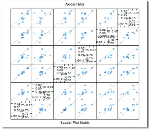
For exploratory analysis, the correlations among the variables were plotted to check if there are any strong collinearity, then a quick decision tree was built on the dataset, and it was observed that the features importance follows this order: glucose, body mass index, age, and number of pregnancies, pedigree, pressure, triceps and insulin.

Figure 2. Correlations among Features

(4)

The relationships between body mass index, pregnancy, disease history and likelihood of the diabetes worth investigating. It was obvious that all these three factors positively indicate diabetes.

Figure 4. Classifying Positive and Negative Cases according to Body Mass Index

Figure 5. Classifying Positive and Negative Cases according to Pedigree

Figure 6. Classifying Positive and Negative Cases according to Pregnancy

VI. EXPERIMENTATION

For measuring performance, the following expressions are used [47]:

True positive (TP): hit.

True negative (TN): correct rejection.

False positive (FP): false alarm or Type I error. False negative (FN): miss or Type II error. Recall (or sensitivity) =

Precision= Accuracy= F-measure=

6.1 LDA

10-fold cross validation has been used for evaluating the model where the dataset is divided into 10 folds. The model is training using nine folds and test is imposed on the tenth, and the then another fold is chosen to be the test portion; this procedure is repeated 10 times. All null values have been replaced with the mean values of the corresponding attributes. The prior probabilities of the groups are 0.651 for negative group and 0.349 for positive groups. The group means and variables coefficients are as following:

Table 2. LDA Group Means

preg nant

gluc ose

pres sure

tric eps

insu lin

mas s

pedi gree

ag e

Neg ative 3.298

109. 98

68.18 4

19.6 64

68.7 92

30.3 042

0.429 734

31. 19 Posit

ive 4.865 672

141. 2575

70.82 463

22.1 6418

100. 3358

35.1 4254

0.550 5

37. 067

Table 3. LDA Coefficients

Variable Coefficient

pregnant 0.093864 glucose 0.026986 pressure -0.01063 triceps 0.000704 insulin -0.00082

mass 0.06037

pedigree 0.671152

(5)

Table 4. LDAConfusion Matrix

Predicted Negative Positive

Actual Negative 442 58

Positive 114 154

Table 5. LDAPerformance Matrix

Model Performance

Accuracy Precision Recall F-measure

77.6% 0.795 0.884 0.837

6.2 Support Vector Machines Model

10-fold cross validation has been used to evaluate the model. RBF kernel function was implemented in the model. The best Gamma value is 0.13; best Cost is 0.25 and number of support vectors is 483.The confusion matrix shows that the precision is slighter better than LDA, but the accuracy, the recall and the overall f-measure have decreased.There are 179 misclassified observations: 68 were wrongly classified as positive and 111 cases were misclassified as negative.

Table 6. Support Vector Machines Confusion Matrix

Predicted Nega tive

Posi tive Ac

tual

Nega tive

432 68

Posit ive

111 157

Table 7. Support Vector Machines Performance Matrix

Model Performance

76.7% 0.796 0.864 0.828

6.3 Naïve Bayes Model

The same 10-fold cross validation is used. The confusion matrix shows that the model accuracy is worse than Support Vector Machine. Nevertheless, the number of misclassified observations as negative is slightly less than those misclassified by SVM. The total number of misclassified observations is 184, 5 cases more than the misclassified SVM cases. The Naïve Bayes precision is the same as the SVM precision, but the recall is less as it registered 0.85 and the total f-measure is 0.822, which is

very close to the SVM f-measure, regardless of the bigger difference in accuracies.

Table 8. Naïve Bayes Confusion Matrix

Predicted Negative Positive Actual Negative 425 75

Positive 109 159

Table 9. Naïve Bayes Performance Matrix

Model Performance

76.04% 0.796 0.85 0.822

6.4 GLMModel

The same 10-fold cross validation is used. The confusion matrix shows that the model accuracy is very close to the LDA model accuracy as it registers 77.47%. The precision is the same as the precision of LDA. Both recall and f-measure are very close to the LDA as their values are: 0.882 and 0.836 respectively. Confusion matrix indicates that the only difference between the two models is the false negative as they are 59 cases in GLM compared to 58 in LDA. Total number of misclassified observations are 173. The GLM model coefficients, confusion matrix and performance matrix are as following.

Table 10. GLM Cofficients

Inter

cept preg

nant gluc ose

pres sure

tric eps

ins ulin

m as s

pedi gree

ag e

-8.405 0.123

0.03 5

-0.013

0.00 1

-0.00 1

0.0 90 0.945

0.0 15

Table 11. GLM Confusion Matrix

Positive 114 154

Table 12. GLM Performance Matrix

Model Performance

Accuracy Precision Recall F-measure 77.47% 0.795 0.882 0.836

6.5 KNNModel

(6)

in accuracy 1.2%. The confusion matrix shows that the model accuracy is obviously worse than SVM, LDA, GLM and NB. Nevertheless, the number of misclassified observations is 210. The accuracy dropped to 72.66% that means that KNN's accuracy is lower than NB's accuracy by 3.39%. The precision, recall and F-measure are equal to 0.771, 0.826 and 0.797 respectively. Therefore, the decrease in f-measure – in comparison to NB – is 0.025 which is less than the decrease in the accuracy metric.

Table 13. KNN Confusion Matrix

Positive 123 145

Table 14. KNN Performance Matrix

Model Performance

6.6Recursive TreeModel

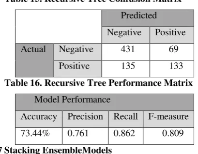
The same 10-fold cross validation is used.The confusion matrix shows that recursive tree model has achieved a better job compared to KNN but still clearly worse that NB. Number of misclassified observations is 204: 69 of them wrongly predicted as positive and the other 135 are incorrectly predicted as negative. The model accuracy is 73.44%, which means a slight increase in accuracy compared to KNN equals to 0.78%. The gap between recursive tree and NB in accuracy is equal to 2.6%. The precision, recall and f-measure equal to 0.761, 0.862 and 0.809 respectively. The f-measure of recursive tree is nearly in the middle between NB and KNN, as the equal to 0.013 and 0.011 respectively. The tree shows that the critical split point as at [glucose<127.5], this rules covers 63% of the dataset, if the condition is not satisfied then the second split point is [BMI>=29.95] which covers 27% of the dataset and [BMI<29.95] covers the rest 10% of the data.

Table 15. Recursive Tree Confusion Matrix

Predicted Negative Positive

Actual Negative 431 69

Positive 135 133

Table 16. Recursive Tree Performance Matrix

Model Performance

6.7Stacking EnsembleModels

The ensemble model is built by stacking all the six models together using a GLM container model and a 10-fold cross validation. Surprisingly the confusion matrix and

the stacking ensemble performance matrix show that the wholistic model yields an accuracy slightly lower than gained from any of the individual LDA, SVM or GLM models.

Table 17. Six Models Stacking GLM Coefficients

Intercept _LDA Recursive _Tree _GLM _KNN _NB _SVM

-2.478

-2.225 -0.525 5.601 0.177 0.385 1.406

Table 18. Six Models Stacking Confusion Matrix

Positive 113 155

Table 19. Six Models Stacking Performance Matrix

Model Performance

76.4% 0.793 0.793 0.793

By checking the correlation among the six models, it is clear that there are some high correlations between some of them. For example, there is a very high correlation between LDA and GLM equals to 0.972. One of these two models should be left out from the ensemble. Therefore, LDA will be kept as it yields a better accuracy. In addition, the correlation between LDA andSVM equals to 0.819. A threshold is set on the correlations, the maximum correlation allowed is set to 0.75, otherwise the model will be left out. Three models are kept after this filtering process: LDA, KNN and Recursive Trees. The tables show the correlation among the models, the new model coefficients,and the three-model stacking ensemble confusion table and performance matrix.

Table 20. Models Correlation

LDA

Recursi

ve Tree GLM KNN SV

M NB

LDA ₁ 0.1883₉₈ 0.972₀₀₄ 0.679₀₄₉ 0.81₉₀₀₄ 0.77₂₈₃₆ Recur

sive Tree

0.188 398 1

0.078 907

0.365 71

0.32 2005

0.21 7603 GLM 0.972₀₀₄ 0.0789₀₇ ₁ 0.636₂₈₇ 0.72₂₃₅₂ 0.77₆₂₂

KNN 0.679₀₄₉ 0.3657₁ 0.636₂₈₇ ₁ 0.81₉₁₃₃ 0.71₂₀₈₁

SVM 0.819₀₀₄ 0.3220₀₅ 0.722₃₅₂ 0.819₁₃₃ ₁ 0.84₅₆₃₃

(7)

Table 21. Three Models Stacking GLM Coefficients

Intercept _LDA Recursive _Tree _KNN

-2.437 4.833 -0.277 0.253

Table 22. Three Models Stacking Confusion Matrix

Positive 18 250

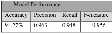
Table 23. Three Models Stacking Performance Matrix

Model Performance

The confusion matrix shows that the stacking ensemble is dramatically enhancing the individual three models. There are only 44 misclassified observations: 26 of them are incorrectly classified as positive and the other 18 are wrongly classified as negative. The accuracy rises to 94.27%, precision, recall and f-measure go up to 0.963, 0.948 and 0.956 respectively. This means that the stacking ensemble added 16.7% to LDA model accuracy and added 0.119 to the f-measure, which is a significant benefit.

VII. CONCLUSION

Stacking ensemble yields the best accuracy and f-measure, it is significantly better than all the individual models. Compared to the LDA which is the best individual model, the ensemble added 16.7% to the accuracy and 0.119 to the f-measure. It is noteworthy, that the correct stacking ensemble is built upon just three models out of the available six models: LDA, Recursive Trees and KNN due to the high correlation among some of the models.

In this study, the stacking ensemble is adopted. In the future, other ensemble techniques worth testing on the six models: bagging, boosting and voting. Then a clear comparison can be made among these four types of ensembles. In addition, the effect of different preprocessing techniques can be studied and the metrics of other important algorithms could be compared such as ANN, Fuzzy Logic and Random Forests.

REFERENCES

[1] Nord, C., Eriksson, M., Dicker, A., Eriksson, A., Grong, E., Ilegems, E., ... & Ahlgren, U. (2016). Multivariate image analysis facilitates label‐free, biochemicalprofiling of the diabetic pancreas. [2] Chatterjee, S., Peters, S. A., Woodward, M., Arango, S. M., Batty,

G. D., Beckett, N., ... & Hassing, L. B. (2016). Type 2 diabetes as a risk factor for dementia in women compared with men: A pooled analysis of 2.3 million people comprising more than 100,000 cases of dementia. Diabetes care, 39(2), 300-307.

[3] Awasthi, A., Parween, N., Singh, V. K., Anwar, A., Prasad, B., & Kumar, J. (2016). Diabetes: Symptoms, Cause and Potential

Natural Therapeutic Methods. Advances in Diabetes and Metabolism, 4(1), 10-23.

[4] Gregg, E. W., Sattar, N., & Ali, M. K. (2016). The changing face of diabetes complications. The Lancet Diabetes & Endocrinology, 4(6), 537-547.

[5] Meier, J. J., & Bonadonna, R. C. (2013). Role of reduced β-cell

mass versus impaired β-cell function in the pathogenesis of type 2

diabetes. Diabetes care, 36(Supplement 2), S113-S119.

[6] Wilding, J. P. H., Woo, V., Rohwedder, K., Sugg, J., & Parikh, S. (2014). Dapagliflozin in patients with type 2 diabetes receiving high doses of insulin: efficacy and safety over 2 years. Diabetes, Obesity and Metabolism, 16(2), 124-136.

[7] Al Jarullah, A. A. (2011, April). Decision tree discovery for the diagnosis of type II diabetes. In Innovations in Information Technology (IIT), 2011 International Conference on (pp. 303-307). IEEE.‏

[8] Dogantekin, E., Dogantekin, A., Avci, D., & Avci, L. (2010). An intelligent diagnosis system for diabetes on linear discriminant analysis and adaptive network based fuzzy inference system: LDA-ANFIS. Digital Signal Processing, 20(4), 1248-1255.‏

[9] Chikh, M. A., Saidi, M., & Settouti, N. (2012). Diagnosis of diabetes diseases using an artificial immune recognition system2 (AIRS2) with fuzzy k-nearest neighbor. Journal of medical systems, 36(5), 2721-2729.‏

[10] Patil, B. M., Joshi, R. C., & Toshniwal, D. (2010, February). Association rule for classification of type-2 diabetic patients. In Machine Learning and Computing (ICMLC), 2010 Second International Conference on (pp. 330-334). IEEE.‏

[11] Jayalakshmi, T., & Santhakumaran, A. (2010, February). A novel classification method for diagnosis of diabetes mellitus using artificial neural networks. In Data Storage and Data Engineering (DSDE), 2010 International Conference on (pp. 159-163). IEEE.‏ [12] Kumari, V. A., & Chitra, R. (2013). Classification of diabetes

disease using support vector machine. International Journal of Engineering Research and Applications, 3(2), 1797-1801.‏ [13] Devi, M. R., & Shyla, J. M. (2016). Analysis of Various Data

Mining Techniques to Predict Diabetes Mellitus. International Journal of Applied Engineering Research, 11(1), 727-730. [14] Wang, S., Lu, J., Gu, X., Du, H., & Yang, J. (2016).

Semi-supervised linear discriminant analysis for dimension reduction and classification. Pattern Recognition, 57, 179-189.

[15] Jia, B., Li, D., Pan, Z., & Hu, G. (2015). Two-Dimensional Extreme Learning Machine. Mathematical Problems in Engineering. [16] Fernando, B., Tommasi, T., & Tuytelaars, T. (2015). Joint

cross-domain classification and subspace learning for unsupervised adaptation. Pattern Recognition Letters, 65, 60-66.

[17] Murthy, K. R., Mondal, A., & Ghosh, A. (2016, November). Maximum Class Boundary Criterion for supervised dimensionality reduction. In Neural Networks (IJCNN), 2016 International Joint Conference on (pp. 4191-4198). IEEE.

[18] Galdi, P., Serra, A., Greco, D., & Tagliaferri, R. (2016, November). Effectiveness of projection techniques in genomic data analysis. In Research and Technologies for Society and Industry Leveraging a better tomorrow (RTSI), 2016 IEEE 2nd International Forum on (pp. 1-6). IEEE.

[19] Dogan, U., Glasmachers, T., & Igel, C. (2016). A unified view on multi-class support vector classification. Journal of Machine Learning Research, 17, 1-32.‏

[20] Amer, M., Goldstein, M., & Abdennadher, S. (2013, August). Enhancing one-class support vector machines for unsupervised anomaly detection. In Proceedings of the ACM SIGKDD Workshop on Outlier Detection and Description (pp. 8-15).‏ [21] Subasi, A. (2015). A decision support system for diagnosis of

neuromuscular disorders using DWT and evolutionary support vector machines. Signal, Image and Video Processing, 9(2), 399-408.‏

[22] Marsland, S. (2015). Machine learning: an algorithmic perspective. CRC press.‏

[23] Buntine, W. L. (2013). Decision tree induction systems: a Bayesian analysis. arXiv preprint arXiv:1304.2732.‏

(8)

[25] Sabry, M. Y., El Kholy, R. B., & Gad, A. M. (2016). Generalized Linear Mixed Models for Longitudinal Data with Missing Values: A Monte Carlo EM Approach. International Journal of Probability and Statistics, 5(3), 82-88.

[26] Luque-Fernandez, M. A., Belot, A., Quaresma, M., Maringe, C., Coleman, M. P., & Rachet, B. (2016). Adjusting for overdispersion in piecewise exponential regression models to estimate excess mortality rate in population-based research. BMC Medical Research Methodology, 16(1), 129.

[27] Strickland, J. (2015). Predictive Analytics Using R. Lulu. com. [28] de Laeuw, J., & Kim, K. (2011). Comparing Four Different

Statistical Packages for Hierarchical Linear Regression: GENMOD, HLM, ML2, and VARCL. Department of Statistics, UCLA. [29] Guisan, A., Edwards, T. C., & Hastie, T. (2002). Generalized linear

and generalized additive models in studies of species distributions: setting the scene. Ecological modelling, 157(2), 89-100.

[30] Hanley, J. A., Negassa, A., & Forrester, J. E. (2003). Statistical analysis of correlated data using generalized estimating equations: an orientation. American journal of epidemiology, 157(4), 364-375. [31] Dornelas, M., Magurran, A. E., Buckland, S. T., Chao, A., Chazdon, R. L., Colwell, R. K., ... & McGill, B. (2013, January). Quantifying temporal change in biodiversity: challenges and opportunities. In Proc. R. Soc. B (Vol. 280, No. 1750, p. 20121931). The Royal Society.

[32] Dramé, K., Mougin, F., & Diallo, G. (2016). Large scale biomedical texts classification: a kNN and an ESA-based approaches. arXiv preprint arXiv:1606.02976.

[33] Adeniyi, D. A., Wei, Z., & Yongquan, Y. (2016). Automated web usage data mining and recommendation system using K-Nearest Neighbor (KNN) classification method. Applied Computing and Informatics, 12(1), 90-108.

[34] Villar, P., Montes, R., Sánchez, A. M., & Herrera, F. (2016, November). Fuzzy-Citation-KNN: a fuzzy nearest neighbor approach for multi-instance classification. In Fuzzy Systems (FUZZ-IEEE), 2016 IEEE International Conference on (pp. 946-952). IEEE.

[35] Jiang, L., Cai, Z., Wang, D., & Zhang, H. (2014). Bayesian citation-KNN with distance weighting. International Journal of Machine Learning and Cybernetics, 5(2), 193-199.

[36] Jaiswal, S., Bhadouria, S., & Sahoo, A. (2015, March). KNN model selection using modified Cuckoo search algorithm. In Cognitive Computing and Information Processing (CCIP), 2015 International Conference on (pp. 1-5). IEEE.

[37] Gouk, H., Pfahringer, B., & Cree, M. (2016). Learning Distance Metrics for Multi-Label Classification. In Proceedings of The 8th Asian Conference on Machine Learning (pp. 318-333).

[38] Hassanat, A. B., Abbadi, M. A., Altarawneh, G. A., & Alhasanat, A. A. (2014). Solving the problem of the K parameter in the kNN classifier using an ensemble learning approach. arXiv preprint arXiv:1409.0919.

[39] Zhang, H., & Singer, B. (2013). Recursive partitioning in the health sciences. Springer Science & Business Media.

[40] Rokach, L., & Maimon, O. (2014). Data mining with decision trees: theory and applications. World scientific.

[41] Kotsiantis, S. B. (2013). Decision trees: a recent overview. Artificial Intelligence Review, 39(4), 261-283.

[42] Howell, C. D. (2015). Tree-based Claims Algorithm for Measuring Pretreatment Quality of Care in Medicare Disabled Hepatitis C Patients.

[43] Feldesman, M. R. (2002). Classification trees as an alternative to linear discriminant analysis. American Journal of Physical Anthropology, 119(3), 257-275.

[44] Kahramanli, H., & Allahverdi, N. (2008). Design of a hybrid system for the diabetes and heart diseases. Expert Systems with Applications, 35(1), 82-89.

[45] Lekkas, S., & Mikhailov, L. (2010). Evolving fuzzy medical diagnosis of Pima Indians diabetes and of dermatological diseases. Artificial Intelligence in Medicine, 50(2), 117-126.

[46] Päivinen, N. (2005). Clustering with a minimum spanning tree of scale-free-like structure. Pattern Recognition Letters, 26(7), 921-930.