University of Pennsylvania
ScholarlyCommons
Publicly Accessible Penn Dissertations
1-1-2016
Discrete Methods in Statistics: Feature Selection
and Fairness-Aware Data Mining
Kory Johnson
University of Pennsylvania, [email protected]
Follow this and additional works at:
http://repository.upenn.edu/edissertations
Part of the
Statistics and Probability Commons
This paper is posted at ScholarlyCommons.http://repository.upenn.edu/edissertations/1788
Recommended Citation
Johnson, Kory, "Discrete Methods in Statistics: Feature Selection and Fairness-Aware Data Mining" (2016).Publicly Accessible Penn Dissertations. 1788.
Discrete Methods in Statistics: Feature Selection and Fairness-Aware Data
Mining
Abstract
This dissertation is a detailed investigation of issues that arise in models
that change discretely. Models are often constructed by either including or
excluding features based on some criteria. These discrete changes are
challenging to analyze due to correlation between features. Feature selection
is the problem of identifying an appropriate set of features to include in a
model, while fairness-aware data mining is the problem of needing to remove
the \emph{influence} of protected features from a model. This dissertation
provides frameworks for understanding each problem and algorithms for
accomplishing the desired goal.
The feature selection problem is addressed through the framework of sequential
hypothesis testing. We elucidate the statistical challenges in repeatedly using
inference in this domain and demonstrate how current methods fail to address
them. Our algorithms build on classically motivated, multiple testing procedures
to control measures of false rejections when using hypothesis testing during
forward stepwise regression. Furthermore, these methods have much higher power
than recent proposals from the conditional inference literature.
The fairness-aware data mining community is grappling with fundamental
questions concerning fairness in statistical modeling. Tension exists between
identifying explainable differences between groups and discriminatory ones. We
provide a framework for understanding the connections between fairness and
the use of protected information in modeling. With this discussion in hand,
generating fair estimates is straight-forward.
Degree Type
Degree Name
Doctor of Philosophy (PhD)
Graduate Group
Statistics
First Advisor
Robert A. Stine
Second Advisor
Dean P. Foster
Keywords
Fairness Aware Data Mining, Feature Selection, Forward Stepwise, Post-Selection Inference, Sequential Testing, Submodular
Subject Categories
DISCRETE METHODS IN STATISTICS: FEATURE SELECTION AND
FAIRNESS-AWARE DATA MINING
Kory D. Johnson
A DISSERTATION
in
Statistics
For the Graduate Group in Managerial Science and Applied Economics
Presented to the Faculties of the University of Pennsylvania
in
Partial Fulfillment of the Requirements for the
Degree of Doctor of Philosophy
2016
Supervisor of Dissertation
Robert A. Stine, Professor of Statistics
Graduate Group Chairperson
Eric Bradlow, K.P. Chao Professor; Professor of Marketing, Statistics, and Education
Dissertation Committee
First Member, Title
Second Member, Title
DISCRETE METHODS IN STATISTICS: FEATURE SELECTION AND
FAIRNESS-AWARE DATA MINING
c
COPYRIGHT
2016
Kory Douglas Johnson
This work is licensed under the
Creative Commons Attribution
NonCommercial-ShareAlike 3.0
License
To view a copy of this license, visit
ACKNOWLEDGEMENTS
I am supremely grateful to my advisors, Bob Stine and Dean Foster, for their many years of
guidance. I often find myself quoting their advice about life and graduate school, and they
have shaped far more than just my research skills. To Dean: for inspiring me to get a PhD
in statistics and to study any topic, regardless of its dubious connection to my research.
To Bob: for being patient with my meandering research interests and providing steady
encouragement and feedback. I owe much of the clarity of this work to his persistence and
mentoring.
I am grateful to the other members of my committee, Lawrence Brown and Andreas Buja,
for our insightful discussions and their insistence that I not move to the next slide unless
they understand every detail on the current one.
I would like to thank my family—Mom, Dad, and Krysta— for your constant love and
encouragement. Your steadfast confidence in my success has always been motivational. To
both my parents and grandparents—Momma Joan and Pop—thank you for believing in
and supporting my education. The opportunities I have had and the flexibility I currently
ABSTRACT
DISCRETE METHODS IN STATISTICS: FEATURE SELECTION AND
FAIRNESS-AWARE DATA MINING
Kory D. Johnson
Robert A. Stine
This dissertation is a detailed investigation of issues that arise in models that change
dis-cretely. Models are often constructed by either including or excluding features based on
some criteria. These discrete changes are challenging to analyze due to correlation between
features. Feature selection is the problem of identifying an appropriate set of features to
include in a model, while fairness-aware data mining is the problem of needing to remove
theinfluenceof protected features from a model. This dissertation provides frameworks for
understanding each problem and algorithms for accomplishing the desired goal.
The feature selection problem is addressed through the framework of sequential hypothesis
testing. We elucidate the statistical challenges in repeatedly using inference in this domain
and demonstrate how current methods fail to address them. Our algorithms build on
clas-sically motivated, multiple testing procedures to control measures of false rejections when
using hypothesis testing during forward stepwise regression. Furthermore, these methods
have much higher power than recent proposals from the conditional inference literature.
The fairness-aware data mining community is grappling with fundamental questions
con-cerning fairness in statistical modeling. Tension exists between identifying explainable
dif-ferences between groups and discriminatory ones. We provide a framework for
understand-ing the connections between fairness and the use of protected information in modelunderstand-ing.
TABLE OF CONTENTS
ACKNOWLEDGEMENT . . . iii
ABSTRACT . . . iv
LIST OF TABLES . . . vii
LIST OF ILLUSTRATIONS . . . ix
CHAPTER 1 : INTRODUCTION . . . 1
CHAPTER 2 : VALID STEPWISE REGRESSION . . . 6
2.1 Inference for Model Selection . . . 11
2.2 Sequential Testing . . . 21
2.3 Polyhedral Selection . . . 32
2.4 Appendix . . . 43
CHAPTER 3 : REVISITING ALPHA-INVESTING . . . 46
3.1 Better Threshold Approximation . . . 49
3.2 Searching Interaction Spaces . . . 55
3.3 Appendix . . . 62
CHAPTER 4 : SUBMODULARITY IN STATISTICS . . . 68
4.1 Submodularity . . . 73
4.2 Submodularity in 2 Dimensions . . . 81
4.3 Connection to Other Assumptions . . . 89
4.4 Appendix . . . 92
CHAPTER 5 : ENSURING FAIRNESS IN ARBITRARY MODELS . . . 95
5.2 Correcting Estimates . . . 123
CHAPTER 6 : DISCUSSION . . . 129
6.1 Valid Stepwise Regression . . . 129
6.2 Submodularity . . . 131
6.3 Fairness-Aware Data Mining . . . 132
LIST OF TABLES
TABLE 1 : Stepwise Regression: Prostate Cancer Data . . . 6
TABLE 2 : Comparison of Holm and BH p-value rejection thresholds. . . 18
TABLE 3 : Simulated critical values under global null. . . 20
TABLE 4 : Stepwise p-values after each step. . . 25
TABLE 5 : Benign correlation structure with minimum eigenvalue .68. . . 27
TABLE 6 : Challenging correlation structure with minimum eigenvalue .18. . . 27
TABLE 7 : Simulation results for Holm, Revisiting Holm, and Forward Stop selection rules.. . . 40
TABLE 8 : Concrete Compression Strength Results. . . 61
TABLE 9 : Simple data in which forward stepwise fails to identify the correct model. . . 68
TABLE 10 : Simplified Loan Repayment data. . . 118
TABLE 11 : Regression Performance . . . 127
LIST OF ILLUSTRATIONS
FIGURE 1 : Illustration of selection and sequential effects under the global null
hypothesis. . . 12
FIGURE 2 : Example of “Revisiting” Holm procedure.. . . 23
FIGURE 3 : Example alpha-investing rules with testing levels. Tests are ordered
numerically and rejections are made at indices 4, 11, 26, 40, and 44. 31
FIGURE 4 : Stepwise rejection regions atα=.1. The full picture is symmetric
around the x- and y-axes. A corresponding image would be drawn
ifZ2 > Z1 >0, in which case the graph would be rotated 90◦ and
maintain its symmetries. . . 35
FIGURE 5 : Small-p results. . . 58
FIGURE 6 : Large-p results. . . 59
FIGURE 7 : Characterization of possible two-dimensional regression problems:
our data consists ofY,X1, and X2. ˆYi isY projected onXi. The
side length from the origin to ˆYi isrY i. . . 82
FIGURE 8 : Contour plot of approximate submodularity using second order
dif-ferences (γs2). Level sets are given forγs2 ∈ {.2, .4, . . . ,2}. . . 84 FIGURE 9 : Contour plot of the left hand side of equation (9). The level sets
are{.2, .4, . . . ,2}. . . 85
FIGURE 10 : This is a contour plot of the submodularity ratio over the set of
fea-sible regression problems. Level sets are given forγsr∈ {.2, .4, . . . ,2}. 86
FIGURE 11 : Contour plot of equation (4.7). The contours interpolate between
.5 and 10 with a step-size of .5. . . 88
FIGURE 12 : A 1936 map of Philadelphia marking high and low-risk areas.. . . 99
FIGURE 14 : Observationally Equivalent Data Generating Models. . . 106
FIGURE 15 : DAGs Using Proxy Variables . . . 111
FIGURE 16 : Veil of Ignorance Hides More Information . . . 116
FIGURE 17 : DAGs of Total Model . . . 121
CHAPTER 1 : INTRODUCTION
This dissertation discusses a variety of methods in seemingly disparate domains. Broadly
speaking, we address issues in model selection, sequential testing, inference after model
selection, and fairness-aware data mining. The last of these may seem disconnected from
the first three; however, it is fundamentally the same problem. All of these topics analyze
the effect of either adding or removing features from a model. This discrete change between
models is complex due to correlation between features.
Chapters2-4analyze the problem of selecting predictive features from a large feature space.
Our data consists ofnobservations of (response, feature) sets, (yi, xi1, . . . , xim), where each
observation has m associated features. Observations are collected into matrices and the
following model is assumed for our data
Y =Xβ+ ∼Nn(0, σ2In) (1.1)
where X is an n×m matrix and Y is an n×1 response vector. Typically, most of the
elements ofβare 0. Hence, generating good predictions requires identifying the small subset
of predictive features. The model (1.1) proliferates the statistics and machine learning
literature. In modern applications, m is often large, potentially withmn, which makes
the selection of an appropriate subset of these features essential for prediction.
The model selection problem is to minimize the error sum of squares
ESS( ˆY) =kY −Yˆk22 =
n
X
i=1
(Yi−Yˆi)2
while restricting the number of nonzero coefficients:
min
β ESS(Xβ) s.t. kβkl0 = m
X
i=1
I{βi6=0} ≤k, (1.2)
not assuming a sparse representation exists, merely asking for a sparse approximation. In
the statistics literature, the model selection problem (1.2) is more commonly posed as a
penalized regression:
ˆ
β0,λ= argminβ{ESS(Xβ) +λkβkl0} (1.3)
whereλ≥0 is a constant. The classical hard thresholding algorithmsCp (Mallows,1973),
AIC (Akaike, 1974), BIC (Schwarz, 1978), and RIC (Foster and George, 1994) vary λ.
The solution to (1.3) is the least-squares estimator on an optimal subset of features. Let
M ⊂ {1, . . . , m}indicate the coordinates of a given model so thatXM is the corresponding
submatrix of the data. If Mλ∗ is the optimal set of features for a given λ then ˆβ0∗,λ =
(XTM∗XM∗)−1XM∗Y.
Given the combinatorial nature of the constraint, solving (1.2) quickly becomes infeasible
asmincreases and is NP-hard in general (Natarajan,1995). Forward stepwise is the greedy
approximation to the solution of (1.2). LetMibe the features in the forward stepwise model
after stepiand note that the size of the model is|Mi|=i. The algorithm is initialized with
M0 =∅and iteratively adds the variable which yields the largest reduction in ESS. Hence,
Mi+1 ={Mi∪j} where
j= arg max
l∈{1,...,m}\Mi
ESS(XMi∪lβˆ LS
Mi∪l).
After the first feature is selected, subsequent models are built having fixed that feature
in the model. M1 is the optimal size-1 model, but Mi for i ≥ 2 is not guaranteed to be
optimal, becauseMi is forced to include the features identified at previous steps.
Conducting valid inference after selecting a model using an algorithm such as forward
stepwise has become a topic of increasing concern. Recently, significant research has been
focused on how to compute appropriate p-values for inference post model selection. Chapter
a model? We want to use hypothesis testing to select one of the models identified by
forward stepwise regression. This is a challenging task because the hypotheses being tested
are suggested by the data and subsequent tests are only made if previous tests are rejected.
Addressing the differences between these two challenges requires increased precision about
the quantity of interest when using hypothesis testing for model selection. Our solution uses
a sequential testing framework and demonstrates that multiple comparison methods can be
adapted to this task. We provide three different procedures to control either the marginal
false discovery rate or the family wise error rate. Furthermore, the resulting methods have
much higher power than those from the conditional inference literature. This extends the
critique of new p-value computations introduced in Brown and Johnson(2016).
Chapter 3 improves upon the methods of Chapter 2, providing several practical
improve-ments which yield an algorithm, Revisiting Alpha-Investing (RAI), which is a fast
approx-imation to forward stepwise. RAI performs model selection in O(nplog(n)) time while
controlling both type-I and type-II errors. As an alpha-investing procedure, it controls
mFDR and is proven to select a model that is a (1−1/e) + approximation to the best
model of the same size. The algorithm is successful under the assumption of approximate
submodularity, which is quite general and allows for highly correlated explanatory variables.
We demonstrate the adaptability of RAI by using it to search complex interaction spaces
in both simulated and real data.
Submodularity plays an important role in the theorems of Chapters 2 and 3 as it
char-acterizes of the difficulty of the search problem of feature selection. The search problem
is the ability of a procedure to identify an informative set of features as opposed to the
performance of the optimal set of features. This is highly important because merely
as-suming that there is a true model which performs well does not entail that a modeler can
find it. Chapter 4 provides a full discussion of submodularity in statistics. Submodular
functions an important function class in optimization which are closely connected to greedy
collinearity makes the choice of model features difficult from those in which this task is
rou-tine. Researchers often report the signal-to-noise ratio to measure the difficulty of simulated
data examples. A measure of submodularity should also be provided as it characterizes an
independent component of difficulty. Furthermore, it is closely related to other statistical
assumptions used in the development of the lasso, Dantzig selector, and sure information
screening.
The feature selection problem is fundamentally concerned with how features can interact
in unexpected ways due to correlation. Here, “unexpected” means that the behavior of a
feature in a model can be completely different depending on the other features included.
One novel domain in which such interactions are highly important is fairness-aware data
mining. This can be viewed as a reverse problem to feature selection in which the modeler
wishes to remove the influence of a feature. Due to correlation between features, merely
excluding the protected feature may leave discriminatory effects which permeate the data.
A simple example clarifies the issue of fairness. Consider a bank that wants to estimate
the risk in giving an applicant a loan. The applicant has “legitimate covariates” such as
education and credit history, that can be used to determine their risk. They also have
“sensitive” or “protected” covariates such as race and gender that society does not want to
be used to determine their risk. The bank’s task is to model the credit risk or credit score
C. To do so, they use historical data, estimate the credit worthiness of the candidate, then
determine the interest rate of the loan. The question asked by FADM is whether or not the
model the bank constructed is fair. This is different than asking if the data are fair or if
the historical practice of giving loans was fair. It is a question pertaining to the estimates
produced by the bank’s model. This generates several questions. First, what does fairness
even mean in this statistical model? Second, what is the role of the sensitive covariates in
this estimate? Lastly, how do we constrain the use of the sensitive covariates in black-box
algorithms?
opposed to discrimination. This stems from imprecise definitions of fairness in statistics.
Chapter 5 provides a detailed account of fairness in statistics by accounting for different
perspectives on the data generating process. This results in a tractable framework for
understanding fairness in modeling as well as algorithms which are guaranteed to provide
fair estimates. These algorithms can be tailored to post-process estimates from arbitrary
models to achieve fairness. This effectively separates prediction and fairness goals, allowing
the modeler to focus on generating highly predictive models without incorporating the
constraint of fairness.
We conclude by discussing the host of new questions raised by this dissertation. As the
sequential testing framework is not part of the statistical cannon, there are many lingering
questions about its ability to solve broader problems. Similarly, fairness-aware data mining
CHAPTER 2 : VALID STEPWISE REGRESSION
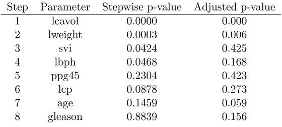
Forward stepwise models can be selected in many ways. To illustrate the use of hypothesis
testing for model selection, consider the prostate cancer data used to motivate the inference
methods of (Taylor et al.,2014). The data set has 67 observations of 8 explanatory variables
which will be used to predict the log PSA level of men who had surgery for prostate cancer.
The traditional use of stepwise regression is summarized in Table 1. Each step of the
procedure adds a feature to the model and assigns a p-value measuring the reduction in
ESS using an F-test. Further information on the construction of the stepwise p-values is
given in the Appendix. The second column of p-values in Table 1 are from Taylor et al.
(2014) and adjust for selecting features using forward stepwise. These adjusted p-values are
introduced in Section2.1.2and discussed at length in Section 2.3.
Our goal is to use the stepwise p-values in Table 1 to determine when to stop forward
stepwise. For example, if it is claimed that the first 4 steps are significant but the 5th is
not, the selected model will include lcavol, lweight, svi, and lbph. Such claims should be
made solely on the basis of the p-values. That being said, attempting to test the addition
of new features uses non-standard and complex distributions (Draper et al.,1971;Pope and
Webster, 1972). Our goal is to provide a valid hypothesis testing framework in order to
select a forward stepwise model.
Table 1: Stepwise Regression: Prostate Cancer Data
Step Parameter Stepwise p-value Adjusted p-value
1 lcavol 0.0000 0.000
2 lweight 0.0003 0.006
3 svi 0.0424 0.425
4 lbph 0.0468 0.168
5 ppg45 0.2304 0.423
6 lcp 0.0878 0.273
7 age 0.1459 0.059
2.0.1. Notation
We use notation from the multiple comparisons literature given its connection to our
solu-tion. Considerm null hypotheses, H[m]: H1, . . . , Hm, and their associated p-values, p[m]:
p1, . . . , pm. The hypotheses can be considered as Hi: βi = 0. Define the statistic Ri = 1
if Hi is rejected and Ri = 0 if not. Similarly, let Viβ = 1 if Ri = 1 is a false rejection (Hi
is true) and Viβ = 0 if not. The dependence of Viβ on β indicates that it is an unknown
quantity which depends on the parameter of interest. For simplicity, the definition below
suppresses this notation. Define
R(m) =
m
X
i=1
Ri, and
V(m) =
m
X
i=1
Viβ
as the total number of rejections and false rejections in them tests, respectively.
One object of concern when testing multiple hypotheses is the family wise error rate
(FWER), which is the probability of making more than one false rejection regardless of
the number of hypotheses tested:
FWER =P(V(m)≥1).
If many hypotheses are tested, controlling the FWER may be too strict. Instead, it is often
more instructive to control the proportion of false discoveries. Our method controls the
marginal false discovery rate (mFDR) which is similar to the more common false discovery
rate (FDR):
Definition 1 (Measures of the Proportion of False Discoveries).
mFDR(m) = E(V(m)) E(R(m)) + 1
FDR(m) =E
V(m)
R(m)
, where 0
In some respects, FDR is preferable to mFDR because it controls a property of a realized
distribution. While not observed, the ratioV(m)/R(m) is the realized proportion of false
rejections in a given use of a procedure. FDR controls the expectation of this quantity.
In contrast, E(V(m))/E(R(m)) is not a property of the distribution of V(m)/R(m). That
being said, FDR and mFDR behave similarly in practice, and mFDR yields a powerful and
flexible martingale (Foster and Stine,2008). This martingale provides the basis for proofs
of type-I error control in a variety of situations.
2.0.2. Contributions
Our first contribution is an elucidation of the effects that must be considered when using
hypothesis testing for model selection. Standard inference tools are invalidated due to two
selection effects: theranking effect and the testing effect. The ranking effect is the result of
testing hypotheses that are suggested by the data and the testing effect is the result of only
conducting future tests if previous tests have been rejected. The impacts of these effects
are explained via example in Section 2.1.
In Section 2.2.1, we demonstrate that the sequential testing approach to multiple
com-parisons yields an approximate forward stepwise algorithm that controls for the selection
effects. Our procedure, Revisiting-Holm (RH), is a threshold approximation to stepwise
regression (Badanidiyuru and Vondr´ak, 2014). At each step, forward stepwise sorts the
p-values of the m0 remaining features, p(1) < . . . < p(m0), and selects the feature with the
minimum p-value, p(1). Instead of performing a full sort, threshold approximations use a
set of increasing rejection thresholds, and hypotheses are rejected when their p-value falls
below a threshold. A feature merely needs to be significantenough, and not necessarily the
most significant. The initial rejection threshold conducts a strict test for which only highly
significant features are added to the model. Subsequent thresholds perform less stringent
tests. As such, the final model is built from a series of approximately greedy choices.
of submodularity. While not often discussed in the statistics literature, submodularity has
important statistical implications and is closely related to more commonly used assumptions
(Johnson et al.,2015c). Submodularity requires that features do not become more significant
when included in a multiple regression than in a simple regression. More generally, consider
a featureXiorthogonal to those in a model,XM. This is referred to as adjustingXiforXM.
The projection operator (hat matrix),HM =XM(XTMXM)−1XTM, computes the orthogonal
projection of a vector onto the span of the columns ofXM. Therefore,Xi adjusted for XM
is denoted Xi.M⊥ = (I−HX
M)Xi. A suppressor variable is one which, once adjusted for,
increases the observed significance of another feature. Submodularity is equivalent to the
absence of conditional suppressor variables, implying that∀M ⊂ {1, . . . , m} andi, j /∈M
|Corr(Y,Xi.(M∪j)⊥)| ≤ |Corr(Y,Xi.M⊥)|.
When this holds, stepwise p-values are non-decreasing as p-values are smaller when features
are considered in smaller models. Clearly the prostate cancer data does not satisfy this;
however, the first several steps have p-values which are non-decreasing. The assumption
of submodularity can be relaxed as discussed in Johnson et al. (2015c), but doing so here
unnecessarily complicates our discussion.
Our first result is proven in Section 2.2.3 by demonstrating that RH is an alpha-investing
procedure (Foster and Stine, 2008). RH is presented independently of alpha-investing so
that the algorithm and proof method are not conflated.
Theorem 1. If the data (Y,X) are submodular andM∗ is the model chosen by
Revisiting-Holm with user defined parameterα, then
E(V(m)) E(R(m)) + 1 ≤α
In some cases, the approximation of RH may be unsatisfactory. Section 2.2.2provides two
the rejection thresholds used by RH as rejection levels for the true stepwise path. This
procedure, “Approximate Revisiting-Holm” (aRH), is conjectured to control FDR under
submodularity. While the martingale proofs of Foster and Stine (2008) are distorted, the
simulations of Section2.3.2support this claim.
Conjecture 1. If the data (Y,X) are submodular andM∗ is the model chosen by
Approx-imate Revisiting-Holm with user defined parameter α, then
E(V(m)) E(R(m)) + 1
≤α
Our construction of RH motivates one final relaxation: using the Holm significance levels
as the rejection thresholds. This is introduced in Section 2.1.2. The resulting procedure,
Stepwise-Holm (SH), is closely related to the Max-|t|procedure ofBuja and Brown (2014)
and controls the FWER under submodularity.
Theorem 2. If the data (Y,X) are submodular and M∗ is the model chosen by
Stepwise-Holm with user defined parameterα, then
P(V(m)≥1))≤α
As noted in Taylor et al. (2014), the Max-|t| procedure can be highly conservative, which
is expected as it controls the FWER. That being said, it performs extremely well in the
simulations of Section2.3.2.
Our framework clearly shows the shortcoming of other procedures recently recommended
in the literature (Taylor et al.,2014). This is discussed at length in Section2.3, where we
demonstrate that classically motivated methods such as RH are preferred. Further evidence
is provided in Section 2.3.2, where RH and its relaxations are shown to have much higher
2.1. Inference for Model Selection
Attempting to use inference for model selection poses significantly different challenges than
merely performing inference after a model is selected. Inference will be conducted multiple
times based on the result of previous inferential claims. Section2.1.1describes two separate
issues raised by such procedures, while Section2.1.2demonstrates that current solutions do
not address both issues.
2.1.1. Selection Effects
We use a simple simulation to demonstrate that it is difficult to provide a valid stepwise
procedure even in the orthogonal case. This separates questions about the statistical validity
of forward stepwise from its ability to approximate the sparse regression problem (1.2). The
model identified at thekth step of forward stepwise exactly solves (1.2) under orthogonality.
The assumption of submodularity guarantees that forward stepwise is both a reasonable
approximation to (1.2) (Nemhauser et al., 1978) and that our methods provide statistical
guarantees. This is discussed in Section2.2.
Suppose the data contain 10 orthogonal explanatory features,β1=. . .=β10= 0, andσ2 is
known. In this case, the test statistics are iidN(0,1) variables but will be called t-statistics
for consistency with data applications. The t-statistics forH1, . . . , H10 are t1, . . . , t10 with
corresponding p-values p1, . . . , p10. The feature selection problem is equivalent to
deter-mining an order for testing H[m] while controlling false rejections at level α. Since our
goal is model selection, a feature is “included” or “added” to the model when the
corre-sponding null hypothesis is rejected. Sort the hypotheses by their absolute t-statistics as
|t(1)| > . . . > |t(10)| (equivalently p(1) < . . . < p(10)). At step i, forward stepwise tests
H(i). In the orthogonal setting, test statistics and p-values do not change depending on the
order in which hypotheses are tested, because coefficients do not change due to the model
in which they are estimated.
(a) (b) (c)
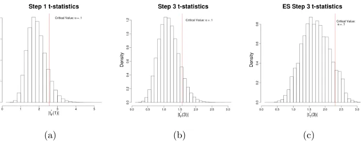
Figure 1: Illustration of selection and sequential effects under the global null hypothesis.
the naive|N(0,1)|. Figure1a and 1b show the distributions of |t(1)|and |t(3)|. Informally,
the difference between these distributions and the distribution of |N(0,1)| is the ranking
effect. This name is motivated as the difference between the test of a rank statistic and a
randomly chosen one. A more precise definition follows shortly.
Since our goal is not to estimate the correct distribution but to perform a valid test, we
desire a critical value yielding a level-αtest. The nominalα=.1 critical value ist= 1.645,
whereas the simulated threshold is t= 2.58. This value can be easily computed using the
Bonferroni correction, and the expected size of further rank statistics can be computed in the
orthogonal case (George and Foster,2000). The .1-critical value for|t(3)|is approximately
1.57, which is lower than the naive level-.1 significance threshold. This is intuitive as |t(3)|
is constrained to be less than |t(2)|by definition.
To be consistent with the standard use of hypothesis testing during forward stepwise, we
propose the procedure “Exact Stepwise (traditional)” (ES-t), that terminates on the first
step in which a hypothesis fails to be rejected using traditional stepwise p-values.1 Such
a perspective is often necessary to allow early termination of an algorithm in large feature
spaces. ES-t only tests H(i) if H(1), . . . , H(i−1) were rejected. On the subset of cases in
which this occurs,|t(i)|is much less constrained, because all of|t(1)|, . . . ,|t(i−1)|were large
1A similar procedure is discussed in Section2.3that uses the methodology ofTaylor et al.(2014) which
enough to be rejected. The distribution of|t(3)|considered by ES-t is only realized on the
subset of cases in which H(3) is actually tested. Figure 1c shows the distribution of |t(3)|
on the subset of cases in which H(1) and H(2) were rejected usingα =.1 under the Holm
method. The Holm method is explained in Section 2.1.2 and entails that p(1) < α/m and
p(2) < α/(m−1). Informally, the difference between the distributions in Figures1b and 1c
is the testing effect. The testing effect increases the simulated critical value from 1.57 to
2.32.
In order to provide precise definitions of the ranking and testing effects, it is necessary
to define different distributions of statistical interest. Classical inference procedures are
interested in controlling the nominal type-I error from a test specified prior to seeing the
data:
PM,H0(reject H0)≤α. (2.1)
Both the modelM and null hypothesis H0 are specified ex-ante and the test is conducted
assuming that the data originate from the model M. If M is misspecified, inference is still
possible though the object of inquiry is the best approximation of the true mean of Y in
the modelM (Buja et al.,2014). Orthogonality breaks the dependence ofH0 onM, as the
presence of other variables does not change coefficient estimates. Most situations are similar
to forward stepwise, in which M and H0 are chosen together, reintroducing dependence.
Therefore, the orthogonal case is still non-trivial.
Often both M and H0 are the result of exploratory data analysis which invalidates the
assumption of pre-specified inference goals. In this case, a reasonable alternative is to
control theselective type-I error (Fithian et al.,2015):
PM,H0(rejectH0|(M, H0) selected)≤α. (2.2)
Given the use of algorithms to identify models, we will separate two different types of
still random as it depends on the data, but the algorithm A does not contain a random
component such as statistical tests. For example, one could test the hypothesis selected on
the third step of forward stepwise. The resulting error is thefixed-selective type-I error:
PFM,H0(rejectH0|(M, H0) selected byA)≤α. (2.3)
The parameters M and H0 are understood to be dependent on the algorithm, A, used in
their identification: M =M(A) and H0 =H0(A). For brevity, this dependence is included
as a superscript in the probability notation.
The testing effect and the discussion in Brown and Johnson (2016) lead us to be more
pedantic in the definition of the selective type-I error rate. We explicitly note the dependence
of the algorithmA on test statisticsT in the definition of thetotal-selective type-I error:
PTM,H0(rejectH0|(M, H0) selected by (A,T))≤α. (2.4)
As before, the parameters M and H0 are understood to be dependent on both the fixed
algorithm,A, and the hypothesis tests, T, used in their identification: M =M(A,T) and
H0 =H0(A,T). For brevity, this notation is included as a superscript in the probability
notation. Acknowledging that test statistics are used to select M does not change the
concept of selective type-I error as the set (A,T) merely produces a meta-algorithm for
performing selection. The difficulty in requiring a completely specified algorithm motivates
the post-selection inference methods ofBerk et al.(2013).
Using the nominal, fixed-selective, and total-selective type-I errors, we can clearly define
the two selection effects which arise when using hypothesis testing for model selection. The
ranking effect is defined as the lack of equivalence between the nominal and fixed-selective
type-I error, and the testing effect is defined as the lack of equivalence between the
Definition 2 (Selection Effects).
Ranking Effect:
PM,H0(reject H0)6=P
F
M,H0(reject H0|(M, H0) selected by A)
Testing Effect:
PFM,H0(reject H0|(M, H0) selected by A)
6
=PTM,H0(reject H0|(M, H0) selected selected by (A,T))
Both selection effects are the result of a selection procedure but are given different names
to separate important distinctions in types of selection. The distinction can be seen by
considering two separate methods to identify a forward stepwise model. The fixed
algo-rithm perspective runs forward stepwise a specified number of steps, then tests the feature
being added. If a stopping condition is used such as selecting the model with minimum
cross-validated error, this must be specified and included in the conditioning. Loftus(2015)
represents such a procedure as a set of constraints on Y in order to condition on the
se-lection event. Therefore,PFM,H0(rejectH0|(M, H0) selected byA) is the appropriate object
of inquiry and coefficients in the final model can be tested via their methods.
Alterna-tively, ES-t can select the forward stepwise model using the p-values in Table1. The model
chosen via this method is the result of repeated hypothesis testing and the correct object
of inquiry is PTM,H0(rejectH0|(M, H0) selected by (A,T)). ES-t requires hypotheses to be
testedsequentially and future tests are influenced by the results of past tests.
2.1.2. Problems with Previous Solutions
Broadly speaking, there are two perspectives on how to account for the selection effects. The
first computes a p-value that corrects for selection. This is a challenging task and is
impossi-ble in some cases. IfM is identified through a model selection procedure,PM,H0(rejectH0)
cannot be estimated (Leeb and P¨otscher,2006). The hypothesisH0 may be specified prior
per-formance measures such as AIC. While this is a common practice, the inability to estimate
PM,H0(rejectH0) renders control of the nominal type-I error impossible.
Estimation is made possible by conditioning on the selection event. Taylor et al. (2014)
control the fixed-selective type I error rate,PFM,H0(reject H0|(M, H0) selected), by specifying
the choice of M via algorithm A as constraints on the response Y. For example, if X1 is
chosen on the first step of forward stepwise, then the t-statistic of ˆβ1 is larger than that
of ˆβi, for i6= 1. This implies a set of linear restrictions on Y. The algorithm A is fixed
and is purely used for optimization as no decisions depend on the result of statistical tests.
Their calculations result in statistics with a uniform distribution underH0, and hence are
called “exact p-values.” The second column of p-values in Table 1are the “exact p-values”
computed using their procedure when forward stepwise is run on the prostate data.
While Taylor et al. (2014) do not explicitly advocate using the p-values as a way to select
models, both the tacit discussion of modeling and the corresponding R package encourage
such a use. One might think that improved p-values would lead to improved model selection,
at least in some circumstances; however, the formulation in Taylor et al. (2014) involves a
serious paradox. One needs to begin with a well-specified model selection algorithm and
construct a model independent of the exact p-values described in the paper. The exact
p-values can be constructed only after the model has been chosen; they cannot validly be
used to select the model. If one tries to use them in this way, they become invalid, because
such tests are not incorporated into the constraints onY. While this does not invalidate the
methodology, it both changes their p-values and significantly hinders computation. This
paradox is also raised in Brown and Johnson (2016) and will be described fully in Section
2.3.
Furthermore, the corresponding package,selectiveInference, suggests selecting models using
procedures fromG’Sell et al.(2015). The independence between between p-values assumed
by G’Sell et al. (2015) is of less concern than the fact that the p-values produced by
selectiveInference must account for the influence of the G’Sell et al. (2015) selection
pro-cedure; however, these procedures are not valid stopping rules, and thus the conditioning
event M(A,T) must encode the entire selection path. The adjusted p-value at stepi
de-pends on the result of calculations from step 1 to the maximum stepm0. We provide more
details and a conservative procedure in Section2.3.2 which allows for early stopping. The
computational cost of incorporating even the simpler constraints implied by the conservative
procedure likely renders it impractical.
The second potential solution to inference for model selection uses traditional, stepwise
p-values but changes the rejection threshold. Multiple comparison procedures such as Holm
(Holm, 1979) and Benjamini-Hochberg (Benjamini and Hochberg, 1995) are of this form.
Bonferroni is a classical, conservative method for controlling for multiple comparisons by
bounding the FWER. Bonferroni changes the rejection threshold from α to α/m, so that
Hiis only rejected ifpi ≤α/m. This controls the FWER by Boole’s inequality. The second
relevant procedure is the Holm step-down method, which proceeds as:
1. Sort the p-values: p(1)< . . . < p(m) and corresponding hypotheses H(1), . . . , H(m).
2. Identifyk= minip(i)> m−iα+1.
3. RejectH(1), . . . , H(k−1).
Holm rejects H(1) if p(1) falls below the Bonferroni level with m hypotheses: α/m. IfH(1)
is rejected, only m−1 hypotheses are still being considered; hence, p(2) is compared to
the Bonferroni threshold using m−1 hypotheses: α/(m−1). This increases the power
of subsequent tests, particularly if many hypotheses are rejected. The final test of H(m)
can even be carried out at the nominal level α. The FWER is controlled according to the
closure principle.
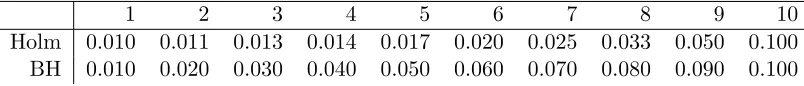
Instead of controlling the probability of making any false rejections, consider controlling
the proportion of false rejections. This provides higher power and may be more appropriate
Table 2: Comparison of Holm and BH p-value rejection thresholds.
1 2 3 4 5 6 7 8 9 10
Holm 0.010 0.011 0.013 0.014 0.017 0.020 0.025 0.033 0.050 0.100
BH 0.010 0.020 0.030 0.040 0.050 0.060 0.070 0.080 0.090 0.100
controls FDR (Benjamini and Hochberg,1995). BH proceeds similarly to Holm:
1. Sort the p-values: p(1)< . . . < p(m) and corresponding hypotheses H(1), . . . , H(m).
2. Identifyk= minip(i)> imα.
3. RejectH(1), . . . , H(k−1)
As in Holm, sorted p-values are compared to a rejection threshold and the algorithm
ter-minates when the threshold is exceeded. Both procedures test p(1) using the Bonferroni
threshold α/m and test p(m) at the nominal level α. BH increases linearly between these
endpoints, providing significantly higher power. Table 2compares the rejection thresholds
of the two methods whenm= 10 and α=.1.
Both the Holm and BH procedures can be improved in the sense that more hypothesis can
be rejected while maintaining control of their respective error criteria. Instead of setting
k as the first time p(k) exceeds the required threshold, set k−1 to be the last time that
p(k−1) is less than the required threshold. We focus on step-down procedures as opposed
to these step-up procedures, because they are similar to sequential methods in that they
provide valid stopping rules. Step-up procedures require all p-values to be computed before
a set of hypotheses can be rejected. This is often unsatisfactory for model selection if there
are many features. For example, the full stepwise path, or at least a predefined maximum
number of steps, must be computed before a model can be identified.
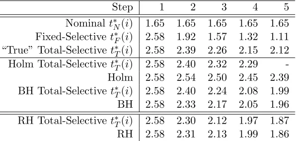
We measure the ranking and testing effects by the difference in critical values for a level-α
test from the different error distributions. In the following display, the notation is simplified
the following critical values:
Nominal threshold: t∗N(i) s.t. PH(i)(|ti|> t
∗
N(i)) =α
Fixed-sequential threshold: t∗F(i) s.t. PHF(i)(|ti|> t
∗
F(i)|H(i)(A) selected) =α
Total-sequential threshold: t∗T(i) s.t. PHT(i)(|ti|> t
∗
T(i)|H(i)(A,T) selected) =α
The nominal thresholdt∗N(i) ignores the selection effects and hence treats all observed
statis-tics asN(0,1). Thus the ranking effect caused by testing hypothesis which are suggested by
the data is measured byt∗N(i)−t∗F(i). For example, |t(1)|is the maximum of 10 t-statistics
and is not distributed as|N(0,1)|. The first step does not demonstrate the testing effect as
no tests have occurred: t∗F(1) =t∗T(1). On subsequent steps, the testing effect is measured
byt∗T(i)−t∗F(i), where the latter accounts for the previous hypothesis tests and the former
does not.
Table3 compares simulated critical values to those generated by Holm and BH forα=.1.
The true fixed-selective critical value, t∗F(i), is merely the .9-quantile of the distribution
of |t(i)|. The true total-selective critical value, t∗T(i), is the .9-quantile of the distribution
of |t(i)| on the subset of cases in which H(1), . . . , H(i−1) were rejected according to some
procedure. Therefore, t∗T(i) depends on the hypothesis testing rule. As identifying the
appropriate rule is the a goal of this paper, we present a couple of different options. The
“true” total-selective t∗T(i) is the critical value if all previous tests are conducted at the
“true” total-selective threshold, where the initial test does not contain the testing effect.
We also showt∗T(i) when hypotheses are tested using Holm, BH, and our proposal, Revisiting
Holm.
First, it is clear that the nominal threshold does not account for the selection effects and
is misleading. The critical value t∗N(i) is initially much smaller than the corrected values,
but quickly becomes larger than t∗F(i) and larger than t∗T(i) for large i. Second, by the
Table 3: Simulated critical values under global null.
Step 1 2 3 4 5
Nominal t∗N(i) 1.65 1.65 1.65 1.65 1.65 Fixed-Selective t∗F(i) 2.58 1.92 1.57 1.32 1.11 “True” Total-Selective t∗T(i) 2.58 2.39 2.26 2.15 2.12 Holm Total-Selective t∗T(i) 2.58 2.40 2.32 2.29
-Holm 2.58 2.54 2.50 2.45 2.39
BH Total-Selective t∗T(i) 2.58 2.40 2.24 2.08 1.99
BH 2.58 2.33 2.17 2.05 1.96
RH Total-Selectivet∗T(i) 2.58 2.30 2.12 1.97 1.87
RH 2.58 2.31 2.13 1.99 1.86
difference is the testing effect and it quickly dominates the rank effect. The intuition for
the magnitude of the testing effect was provided previously: on the subset of cases in which
H(i) is tested by ES-t,|t(i−1)|does not place a strong constraint on|t(i)|. The relative sizes
of the selection effects is troubling as the conditional methods ofTaylor et al.(2014) ignore
the testing effect.
Third, there are large differences between the simulated critical values and those produced
using the corresponding multiple comparison methods. While the procedures control very
different error measures, it is instructive that neither method estimates the corresponding
total-selective critical value correctly. This demonstrates the need for a new method
ac-counting for the ranking and testing effects. Lastly, the bottom two rows show the critical
values produced by our approximate stepwise procedure Revisiting Holm. The computed
values match the simulated critical valuest∗T(i).
As we demonstrate in Section 2.2, sequential testing fits somewhere between the two
po-tential solutions discussed in this section. We use stepwise p-values such as those from
Table 1 to craft an algorithm which looks like a multiple comparison procedure; however,
an important update occurs between tests which changes the “effective” testing level. This
update also accounts for the differences between the RH total-selectivet∗T(i) and the “true”
2.2. Sequential Testing
The Revisiting Holm procedure (RH) is motivated by controlling multiple comparisons in
a sequential testing framework. Sequential testing assumes the hypotheses H[m] arrive
sequentially. As such, the current hypothesis must be tested before observing subsequent
hypotheses. This leads to a new mindset for multiple comparison control as well as corrected
rejection thresholds for inference for model selection. While the corrections are only exact
in the orthogonal case, we demonstrate that they are robust to certain deviations from
orthogonality. Furthermore, the simulations in Section2.3.2demonstrate that RH controls
FDR in nonorthogonal cases and has much higher power than competitors.
2.2.1. Approximating Stepwise Regression
At each iteration, forward stepwise sorts the stepwise p-values of all remaining features in
order to select the feature with the minimum p-valuep(1). Instead of performing a full sort,
consider using increasing rejection thresholds, where hypotheses are rejected when their
p-value falls below a threshold. For now, set aside the concern about type-I error control to
focus on the order in which covariates are selected by RH. Consider thresholds determined
by the Holm step-down procedure. The approximate stepwise algorithm is:
1. TestH(1), . . . , H(m) at levelα/m.
2. Ifp(1)> α/m, stop with no rejections, else rejectH(1). This was the first “pass” through
the features or “round” of testing. For now, assume that only one rejection is made on
this pass, ie, p(2)> α/m.
3. TestH(2), . . . , H(m)at levelα/(m−1), following the rejection procedure as before. Again,
assume only one rejection.
4. Continue making testing passes using the Holm thresholds until all remaining hypotheses
fail to be rejected in a round, then terminate. The selected model includes the variables
While this looks identical to the original Holm procedure, there is an important distinction:
hypotheses are formally tested multiple times. Therefore, the procedure must condition on
the results of previous tests.
To introduce the implications of this conditioning, consider a level-α test with rejection
threshold p∗. In general, α and p∗ are not discussed of as two separate parameters,
be-cause they are equal when the p-value is uniformly distributed and unconstrained. When
conditioning on the result of previous tests, however, they are different.
Definition 3 (Level-α test, rejection thresholdp∗).
PH0(p≤p
∗
) =α ⇒ Standard case: p∗ =α
When testing a hypotheses on the second round, one must account for the failed test in the
first round. In our simulation example withm = 10 andα =.1, the second pass performs
a level-.01/9 test conditional on the p-value being greater than the first pass threshold of
.1/10. Under the null hypotheses, the sequential p-value is uniformly distributed; hence the
thresholdp∗ can be computed as
.1/9 =Pnull(p2 ≤p∗|p2 > .1/10) (2.5)
= p
∗−.1/10
1−.1/10
⇒p∗ = 0.021.
Intuitively, the Holm testing level is an allocation of error probability. The rejection
thresh-old with error probability .1/9 is not .1/9 given the failed test on the first pass. Revisiting
Holm uses rejection thresholds which account for testing hypotheses multiple times. It
formally revisits hypotheses and is named for this characteristic. (Foster and Stine, 2008)
note that this procedure produces thresholds similar to BH, while this paper extends their
discussion to model selection and points to additional benefits. The practical benefits of
2 4 6 8 10
0.00
0.05
0.10
0.15
0.20
0.25
0.30
Revisiting Holm
Index
p-values
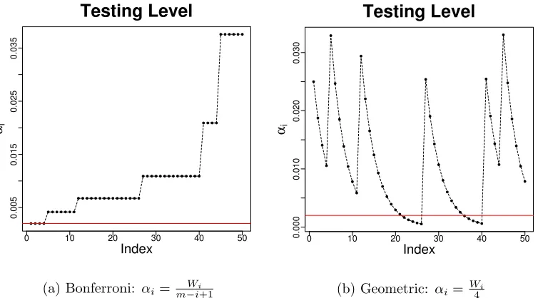
Figure 2: Example of “Revisiting” Holm procedure.
(2015b).
For clarity, Figure 2 shows a few steps of RH. Our hypothetical data follows the simple
simulation example with 10 orthogonal explanatory variables and α = .1. The rejection
thresholds during the first four passes are the horizontal, dashed lines. The first step of
the procedure tests all p-values at level .1/10. As one p-value falls below this threshold, its
hypothesis is rejected and the procedure continues. Step 2 tests the remaining hypotheses at
level-.1/9 which leads to a rejection threshold of .021. One p-value is below this threshold, so
its hypothesis is rejected and the procedure continues. Step 3 tests the remaining hypotheses
at level-.1/8 and rejection threshold .033, which leads to a third rejection. Step 4, however,
fails to make any rejections using a rejection threshold of .047. Therefore the algorithm
terminates, resulting in the model selected during the first 3 steps: features 2, 4, and 6.
If only one hypothesis is rejected per round, then RH exactly replicates the forward stepwise
selection path. To relax this assumption, suppose that both p(1) < α/m and p(2) < α/m
such that both hypotheses would be rejected on the first pass. Since H(1) was rejected,
H(2) could be tested at level-α/(m−1). Such a test has higher power, but was ultimately
This early rejection results in two effects. First, the early rejection changes the reference
distribution for the second testing pass. RH is not attempting to test all possible H(2) on
the second pass, but merely those that were not rejected on the first pass. Therefore, the
simulated total-selective critical value for RH should only be computed from the subset of
cases in which H(i) was not already rejected in a previous pass. This excludes those cases
where p(i) < t∗T(i−1). The result of this change is seen in Table3. RH produces critical
values that are effectively identical to the simulated total-selective values t∗T(i).
Second, if multiple hypotheses are rejected in a round, RH is not guaranteed to have selected
the most significant feature first. Since the features were not truly sorted, it is unknown
which of the two hypotheses rejected in the first pass actually had a smaller p-value. Both
p-values were merely smaller than α/m. In this case, the order in which the hypotheses
are tested is influential. If H(2) is tested before H(1), then RH includes the corresponding
features X(1) and X(2) in the wrong order.
Selecting features in the wrong order is not of serious concern in the orthogonal case,
because the same set of features will have been selected by the end of each testing pass. In
nonorthogonal settings, however, test statistics change based on the model in which they are
computed, so selecting features in a different order can lead to significantly different models.
This is easiest to see by example. Table 4 gives the sequential p-values of all features in
the prostate cancer data in different selected models. Two algorithms are compared: RH
testing the features in sorted stepwise order 1-8 (RH-sort), and RH testing the features in
the reverse order 8-1 (RH-rev). The reverse order provides a worst-case ordering for RH.
In the table, hyphens indicate the features in the model.
Forward stepwise, RH-sort, and RH-rev consider the same p-values initially (step 0), as
no features have been added to the model. These p-values are computed from simple
regressions between the response and the feature of interest using an independent estimate
of the error variance. While all features fall below the RH threshold, lcavol has the lowest
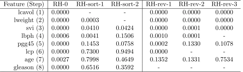
Table 4: Stepwise p-values after each step.
Feature (Step) RH-0 RH-sort-1 RH-sort-2 RH-rev-1 RH-rev-2 RH-rev-3
lcavol (1) 0.0000 - - 0.0000 0.0000 0.0000
lweight (2) 0.0000 0.0003 - 0.0000 0.0000 0.0000
svi (3) 0.0000 0.0410 0.0424 0.0000 0.0001 0.0000
lbph (4) 0.0006 0.0041 0.1506 0.0010 0.0001
-pgg45 (5) 0.0000 0.1453 0.0758 0.0002 0.1330 0.1078
lcp (6) 0.0000 0.7300 0.9494 0.0000 -
-age (7) 0.0027 0.7998 0.4649 0.1352 0.1331 0.7534
gleason (8) 0.0000 0.6516 0.3592 - -
-p-values in the column RH-sort-1 are the stepwise -p-values given that lcavol is in the model.
Again, RH-sort and forward stepwise select the same variable, lweight, at the second step.
Adjusting the stepwise p-values for the model (lcavol, lweight) results in the column
RH-sort-2. All of these p-values fall above the RH threshold for the third testing pass, so the
procedure terminates. The correspondence between RH-sort and forward stepwise seen here
is a general property: if RH tests variables in the order determined by stepwise, then RH
selects variables in the same order as stepwise.
RH-rev behaves significantly differently than RH-sort and forward stepwise. The initial
p-values it considers are identical, but RH-rev tests gleason first and the test is rejected. The
p-values in the column RH-rev-1 condition on gleason being in the model. Proceeding in the
reverse order, the test of age is not rejected, but the test of lcp is. Column RH-rev-2 updates
the stepwise p-values given the model contains gleason and lcp. Using these p-values, lbph
is also rejected, and the process continues. In fact, RH-rev rejects all 8 features. Given
the ordering of the features this is at least justifiable. Each subsequent feature explains a
significant reduction in ESS. Even after several features are in the model, lcavol provides
unique information about the response. That being said, selecting all 8 features is clearly
not desirable and motivates the relaxations of Section 2.2.2. Alternatively, by choosing a
different set of rejection thresholds Johnson et al. (2015b) mimic stepwise regression very
well. In this case, their method selects the RH-sort model of {lcavol, lweight}regardless of
In nonorthogonal data, one may object to the updating in equation (2.5) because sequential
p-values are relevantly different between steps. While the same explanatory feature is being
tested, the sequential p-value is a function of the other variables in the model. For example,
if other hypotheses were rejected between two tests ofHi, there is, in general, no guarantee
that the conditioning statement in equation (2.5) is accurate; a feature can become more
significant in the presence of other features. This is seen in Table6and discussed at length
inJohnson et al. (2015c). Three considerations alleviate this concern. First, the extent to
which p-values can change in the presence of other variables is controlled by the approximate
submodularity of the data Johnson et al.(2015b). In fact, the statement is conservative if
the data are submodular. The degree of approximate submodularity can be bounded by
the minimum eigenvalue of the covariance matrix ofX. Dependence is not measured by the
correlation between variables because not all correlation is problematic for model selection.
Second, the simulation in Section 2.3.2 demonstrates that deviations do not harm type-I
error control. Third, the significance thresholds developed inJohnson et al.(2015b) render
the critique obsolete, in that the correction in equation (2.5) makes a minuscule change
to the effecting testing level. The correction can be ignored with a minimal reduction in
power.
We provide two simulated examples using correlated data to demonstrate the behavior of RH
in more difficult scenarios. RH provides a good approximation of true critical values under
mild dependence, but extreme dependence degrades the approximation. As shown in Section
2.3.2, even conservative competitors can be broken in these cases. We directly simulate the
distribution of 10 t-statistics as done in the original simulations of this section. The first
simulation example has a benign correlation structure where the correlation between indices
iand j is.2|i−j|. The minimum eigenvalue of the corresponding data matrix is .68.
The second simulation example has a challenging correlation structure in which the
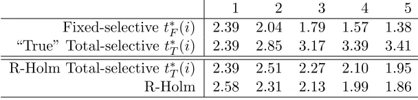
corre-lation between indicesiand jis.8|i−j|. This results in the strange effects in Table6, where
Table 5: Benign correlation structure with minimum eigenvalue .68.
1 2 3 4 5
Fixed-selectivet∗F(i) 2.56 1.93 1.58 1.33 1.12 “True” Total-selective t∗T(i) 2.56 2.43 2.30 2.20 1.98 R-Holm Total-selective t∗T(i) 2.56 2.32 2.15 2.01 1.90
R-Holm 2.58 2.31 2.13 1.99 1.86
feature on the first step. Therefore, given this one feature model, it is possible for a feature
to appear even more significant than the initially most significant feature. This reversal
produces effects such as insignificant steps followed by significant ones. While RH does not
approximate the total-selective critical value as well, the deviations are not extreme. This
allows it RH to maintain performance measures in the simulations of Section 2.3.2.
Table 6: Challenging correlation structure with minimum eigenvalue .18.
1 2 3 4 5
Fixed-selectivet∗F(i) 2.39 2.04 1.79 1.57 1.38 “True” Total-selective t∗T(i) 2.39 2.85 3.17 3.39 3.41 R-Holm Total-selective t∗T(i) 2.39 2.51 2.27 2.10 1.95
R-Holm 2.58 2.31 2.13 1.99 1.86
2.2.2. Relaxations
The dependence of RH on the order in which features are tested may be impractical or
unsatisfactory for some applications. This subsection introduces two relaxations that can
be validly used to identify a model using a stepwise table such as Table1. The first relaxation
makes the tacit assumption that only one hypothesis is rejected per round. In this case,
RH selects the same features in the same order as forward stepwise. Furthermore, the RH
critical values accurately describe the forward stepwise table. The approximate procedure,
aRH, operates as follows:
1. Compute a stepwise table where the sequential p-value for stepiispi. The p-values are
not necessarily sorted: pi need not be less than pj ifi < j.
crh(1) =α/m,
crh(i) =crh(i−1) +α/(m−i+ 1)−crh(i−1)α/(m−i+ 1) fori >1.
This follows from the conditioning in equation (2.5).
3. Identifyk= minipi > crh(i).
4. RejectH(1), . . . , H(k−1).
Foster and Stine (2008) point out that crh are initially close to the Benjamini-Hochberg
thresholds iα/m. Conjecture 1 suggests that aRH controls mFDR and is substantiated by
the simulations in Section 2.3.2. Clearly the claim is true if only one sequential p-value is
rejected per round as aRH and RH coincide. The proof of this claim is less important as
further revisions to RH yield a revisiting procedure, Revisiting Alpha-Investing, which is
proven to closely mimic forward stepwise (Johnson et al.,2015b). The authors also explain
and develop further practical benefits of using a precise threshold approximation to stepwise
regression.
A final relaxation is of independent theoretical and practical interest. Given the discussion
at the end of Section 2.2.1, one may question the update implied by revisiting in equation
(2.5). In particular, if the data is not submodular, then there is no guarantee that a
p-value does not decrease in the presence of other variables. A conservative statement is
provided by ignoring the revisiting component of RH. Namely, merely use the Holm levels
as the rejection thresholds for each testing pass on a given stepwise table. The resulting
procedure, Stepwise-Holm (SH), proceeds as follows:
1. Compute a stepwise table where the sequential p-value for stepiispi. The p-values are
not necessarily sorted: pi need not be less than pj ifi < j.
2. Identifyk= minipi > α/(m−i+ 1).
3. RejectH(1), . . . , H(k−1).
SH extends the intuition behind the Max-|t|procedure of Buja and Brown(2014). Under
2 is given in the Appendix. While this controls false rejections in a conservative way, SH
performs well in the simulations of Section 2.3.2.
As pointed out inTaylor et al.(2014), the conservatism of SH is in part due to the ranking of
test statistics, ie|t(3)|is constrained to be less than|t(2)|. That being said, their discussion
is incomplete because it ignores the testing effect. Furthermore, as shown in Section 2.2.1,
the t-statistics of subsequent steps need not be smaller than those of previous steps in
non-orthogonal cases. This complicates the analysis because merely observing an insignificant
variable is not sufficient indication that there is no signal left in the data. Such instances
form the core problem cases for feature selection algorithms and are discussed at length in
Johnson et al. (2015c).
2.2.3. Alpha-Investing
RH is closely connected to commonly used multiple comparison procedures which alludes
to its type-I error control. This control is proven by demonstrating that the procedure is
an alpha-investing rule (Foster and Stine,2008). Alpha-investing rules are similar to
alpha-spending rules in that they are given an initial amount of alpha-wealth which is spent on
hypothesis tests. Wealth is the total allotment of error probability. Bonferroni allocates
this error probability equally over all hypothesis, testing each one at levelα/m. In general,
the amount spent on tests can vary. Ifαi is the amount of wealth spent on testHi, FWER
is controlled when
m
X
i=1
αi ≤α.
In clinical trials, alpha-spending is useful due to the varying importance of hypotheses.
For example, many studies include both primary and secondary endpoints. The primary
endpoint of a drug trial may be determining if a drug reduces the risk of heart disease.
As this is the most important hypothesis, the majority of the alpha-wealth can be spent
on it, providing higher power. There are often many secondary endpoints such as testing
remaining wealth equally over the secondary hypotheses. FWER is controlled and the
varying importance of hypotheses is acknowledged.
Alpha-investing rules are similar to alpha-spending rules except that alpha-investing rules
earn a return, or contribution to their alpha-wealth, of ω ≤ α when tests are rejected.
Therefore, the alpha-wealth after testing hypothesis Hi is
Wi+1 =Wi−αi+ωRi
An alpha-investing strategy uses the current wealth and the history of previous rejections
to determine which hypothesis to test and the amount of wealth that should be spent on it.
Intuitively, alpha-investing rules spend error probability in search of false null hypotheses
to reject. Each false null that is rejected allowsα more incorrect rejections in expectation.
Alpha-investing rules merely need to spend more wealth (error probability) than the
prob-ability of error they incur. In some sense, this behavior is present in all procedures which
control a proportion of false rejections. For example, if it is known that the first 9
rejec-tions were of false hypotheses, then any 10th hypothesis can be rejected while controlling
the proportion of false rejections at .1.
We provide two examples of potential spending rules. The first is similar to Bonferroni
in that wealth is spent evenly over all remaining hypotheses. Note that this requires the
number of hypotheses to be known in advance. Given current wealth Wi, this procedure
spends
αi = Wi m−i+ 1
to testHi. Figure3ashows the testing levels of this rule with starting wealthW1=.1 when
testing a set of 50 hypotheses in which rejections are made on tests 4, 11, 26, 40, and 44.
The procedure begins by testing at the usual Bonferroni level with m = 50, but rejections
0 10 20 30 40 50
0.005
0.0
15
0.025
0.035
Testing Level
Index αi
(a) Bonferroni: αi=m−Wii+1
0 10 20 30 40 50
0.000
0.010
0.020
0.030
Testing Level
Index αi
(b) Geometric: αi= W4i
Figure 3: Example alpha-investing rules with testing levels. Tests are ordered numerically and rejections are made at indices 4, 11, 26, 40, and 44.
The second example is a geometric spending rule that allows the total number of hypotheses
to be unknown. In this case, the alpha-investing rule merely spends one quarter of its current
wealth on the current test: αi = Wi/4. This spends wealth rapidly following a rejection
and is sensible if false hypotheses are anticipated to arrive in groups. Figure3b shows the
testing levels in the same scenario considered for the Bonferroni strategy. One important
difference between the procedures is that the Bonferroni rule spends all of its wealth by
the end of the 50 tests whereas the geometric rule does not. The geometric procedure is
also related to a universal strategy. If tests only arrive sequentially without being revisited,
there exists a strategy that cannot be outperformed by a significant margin by any other
strategy. This universal procedure is an adaptively weighted set of geometric strategies
(Foster et al.,2001).
Viewing the Holm step-down procedure as an alpha-investing rule creates the Revisiting
Holm procedure and proves its control of mFDR. Given initial alpha-wealth α and return
ω = α, test all hypotheses at the Bonferroni level, α/m. This exhausts all alpha-wealth,