A Supervised Classification Method for Levee Slide Detection Using Complex Synthetic Aperture Radar Imagery

(1)

Concept Paper

A Supervised Classification Method for Levee Slide

Detection Using Complex Synthetic Aperture

Radar Imagery

Ramakalavathi Marapareddy 1,_{*, James V. Aanstoos}2_{and Nicolas H. Younan}3

1 _{Center for Advanced Vehicular Systems, Mississippi State University, Mississippi State, MS 39759, USA}

2 _{Geosystems Research Institute, Mississippi State University, Mississippi State, MS 39759, USA;}

[email protected]

3 _{Department of Electrical and Computer Engineering, Mississippi State University, Mississippi State,}

MS 39762, USA; [email protected]

* Correspondence: [email protected] or [email protected]; Tel.: +1-662-325-2057

Abstract: The dynamics of surface and sub-surface water events can lead to slope instability resulting in anomalies such as slough slides on earthen levees. Early detection of these anomalies by a remote sensing approach could save time versus direct assessment. We have implemented a supervised Mahalanobis distance classification algorithm for the detection of slough slides on levees using complex polarimetric Synthetic Aperture Radar (polSAR) data. The classifier output was followed by a spatial majority filter post-processing step which improved the accuracy. The effectiveness of the algorithm is demonstrated using fully quad-polarimetric L-band Synthetic Aperture Radar (SAR) imagery from the NASA Jet Propulsion Laboratory’s (JPL’s) Uninhabited Aerial Vehicle Synthetic Aperture Radar (UAVSAR). The study area is a section of the lower Mississippi River valley in the southern USA. Slide detection accuracy of up to 98 percent was achieved, although the number of available slides examples was small.

Keywords: Synthetic Aperture Radar; UAVSAR; levee; classification; radar polarimetry;

classification

1. Introduction

Earthen levees protect large areas of populated and cultivated land in the United States from flooding. The potential loss of life and property associated with the catastrophic failure of levees can be extremely large. Over the entire US, there are more than 150,000 kilometers of levee structures of varying designs and conditions. One type of problem that occurs along these levees, which can lead to complete failure during a high water event if left unrepaired for too long, is a slough slide [1]. Slough slides are slope failures along a levee, which leave areas of the levee vulnerable to seepage and failure during high water events [2]. The roughness and related textural characteristics of the soil in a slide area affect the amount and pattern of radar backscatter. The type of vegetation that grows in a slide area differs from the surrounding levee vegetation, which can also be used in detecting slides [3].

(2)

of a scattering matrix are related to the properties of the target, several decomposition methods based on the scattering matrix have been proposed to identify target scattering characteristics [7-8]. Kong et al. [9] proposed an optimal polarimetric classifier based on the complex Gaussian distribution with single-look data. Lee et al. [10] proposed a maximum likelihood classifier of multi-look SAR data based on the complex Wishart distribution, and also an improved method using unsupervised classification combined with the H/alpha decomposition [11]. Cloude and Pottier introduced [12] the entropy-alpha-anisotropy (H/α/A) classification based on the eigenvalues of the polarimetric (or coherency) covariance matrix.

The magnitude data itself may be sufficient for the classification of targets, but this data alone may not be enough to describe the complete structure of the targets. The phase data also has very useful information about the target details. In this paper, we implemented a supervised classification algorithm for the identification of slough slides on levees using the magnitude, phase, and complex data (magnitude and phase) ofpolSAR imagery. The classification result was further followed by a majority filter, which improved the classification accuracy. Higher classification accuracy for the complex data is obtained when compared with the magnitude and phase classification alone.

Three different sample area segments, which each contain at least one active slide, are used for the analysis. The effectiveness of the presented method is demonstrated using fully quad-polarimetric L-band SAR imagery from the NASA JPL’s UAVSAR.

2.

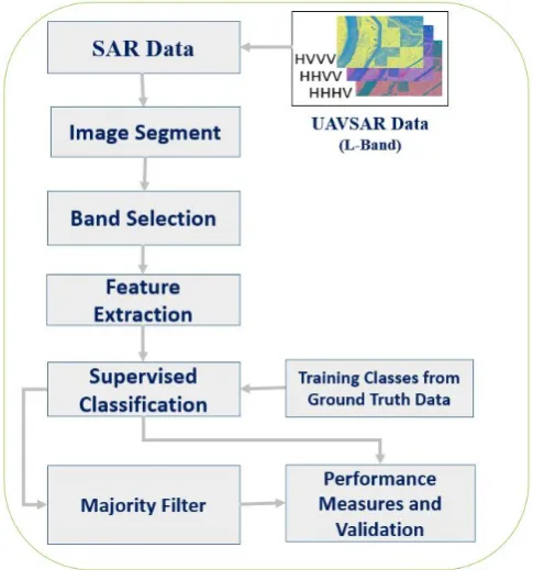
Method

(3)

Figure 1. Processing steps for slide detection on levee. 2.1 Data and Study Area

The study area for this work focuses on the mainline levee system of the Mississippi River along the eastern side of the river in Mississippi, USA. This study used airborne L-band polSAR data acquired by NASA JPL’s UAVSAR instrument. The L-band radar is capable of penetrating dry soil to few centimeters depth. Thus, it is valuable in detecting changes in levees that are key inputs to a levee condition classification system [13].

The data set consists of the HHHV, HHVV, and HVVV MLC, as well as individual polarization channel magnitude and phase data. The MLC data consists of 3 sets of complex floating points values. These complex products are derived from an average of 3 pixels in range and 12 pixels in azimuth, i.e., the number of range looks in MLC and number of azimuth looks in MLC are 3x12 of the product of each SLC pixel, which correspond to HHHV, HHVV, and HVVV. The slant range pixel spacing for the MLC data is by 7.2m x 4.99m for the azimuth and range directions, respectively. The pixel spacing for the SLC data is by 0.6m x 1.66m for the azimuth and range directions, respectively. The SLC data sets (HH, HV, and VV) are oversampled in nature and are dominated by speckle noise. We chose the MLC data sets to reduce the speckle effects. For the MLC data used, the projected ground sample distance is of size 5.5m by 5.5m.

(4)

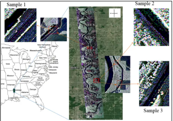
Figure 2. Study area with radar color composite 3 band (HH, VV, & HV) image overlaid on base map.

2.2 Training Data

The availability of ground truth data for training the supervised classification processes is a challenge since the targets of interest are portions of the levee that show signs of impending failure. Once these are detected, they are quickly repaired depending on their severity [14]. The study area is one in which the levees are managed by the US Army Corps of Engineers (USACE) and are well-monitored. The Corps, in association with the local levee boards, maintains a good cumulative history of past problems and has identified particularly problematic sections of levees in the study area as shown in Table 1. These are used as training samples [13]. In addition to the ground truth data provided by the Corps, we have conducted field trips at the time of image acquisition to visually inspect the slides area and levee condition. The active slides (slides 1, 2, and 5) were present and unrepaired during the radar image acquisition time on January 25, 2010. Though the date of slide appearance was not identified by the Corps for slide 5, it is visible in the NAIP (National Agriculture Imagery Program) imagery collected in 2009 and 2010, and was not repaired until after the image acquisition as shown in Table 2. Hence, it was an active slide during the time of the image. Training masks were created for the slide events and labeled as either repaired or unrepaired at the time of acquisition. The training sample data from slide and nonslide (healthy) parts of the levees were obtained from the radar data using the training masks for analysis. The samples from the healthy parts of the levee near the slide events were used for training of the nonslide (healthy levee) class.

Table 1. Ground truth data from Mississippi Levee Board.

Slide Number Length Vert. Face Dist. from Crown Latitude North Longitude West Date Slide Appeared Date Slide Repaired

1 135' 15' 12'

N33-07'-44.4"

W91-04'-46.1"

Oct. 2009 Mar. 2010

2 230' 7' 9'

N32-37'-37.2"

W90-59'-56.2"

Oct. 2009 Apr. 2010

3 80' 2' 30'

N32-36'-37.7"

W90-59'-42.3"

Oct. 2009 Nov. 2009

4 120' 3' 15'

N32-36'-32.0"

W90-59'-46.3"

Aug. 2008 Nov. 2009

5 200' 8' 8'

N32-36'-29.1"

W90-59'-48.0"

(5)

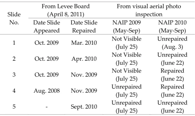
Table 2. Updated slides ground truth from Mississippi Levee Board.

Slide No.

From Levee Board (April 8, 2011)

From visual aerial photo inspection Date Slide Appeared Date Slide Repaired NAIP 2009 (May-Sep) NAIP 2010 (May-Sep)

1 Oct. 2009 Mar. 2010 Not Visible (July 25)

Unrepaired (Aug. 3)

2 Oct. 2009 Apr. 2010 Not Visible (July 25)

Unrepaired (June 22)

3 Oct. 2009 Nov. 2009 Not Visible (July 25)

Repaired (June 22)

4 Aug. 2008 Nov. 2009 Unrepaired (July 25)

Repaired (June 22)

5 - Sept. 2010 Unrepaired

(July 25)

Unrepaired (June 22)

2.3 Mahalanobis distance classification

The Mahalanobis distance is a direction sensitive distance classifier that uses statistics for each class in a manner similar to the maximum likelihood classifier but it assumes all class covariances are equal and weighing factors are not required [15-16]. Therefore, it is a faster method. The Mahalanobis distance algorithm is similar to the minimum distance algorithm, except that it uses the covariance matrix instead. It can be more useful than the minimum distance in cases where statistical criteria are taken into account and it is largely based on a normal distribution of the data in each band which is used as input to classification [17]. Unlike the minimum distance, this method takes the variability of classes into account. The maximum distance error can be a zero threshold for all the classes, or singlevalue (0 to 0.9) for all the classes, or different values (0 to 0.9) for individual classes. The distance threshold is the distance within which a class must fall from the center or mean of the distribution for a class. We used a zero threshold for all the classes. The Mahalanobis distance classification calculates the distance for each pixel in the image to each class using the following equation [15]:

= − ∑ − (1)

where:

D =Mahalanobis distance i = the ith_class

x = n-dimensional data (where n is the number of features) Σ-1_{= the inverse of the covariance matrix of a class}

= mean vector of a class 4. Results and Discussion

The Mahalanobis distance supervised classification process was run separately with the magnitude only, phase only, and full complex (magnitude and phase) SAR multi-looked cross product data on each of the three sample images. The cross-polarized products, HHHV, HHVV, and HVVV, are used based on the assumption that they carry more information about relevant surface scattering properties than the co-polarized channels.

Using the reference (ground truth) data, image masks were created bounding the active slide area and a subset of the non-slide area within each sample image. A sample of the pixels in of each of these two classes was then used to train the classifier. The accuracy of the resulting classification was tested using the remaining reference data pixels for testing, and the conventional statistics of user producer, and overall accuracy were computed for each case.

(6)

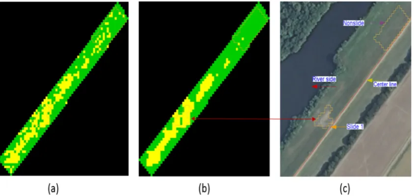
132 pixels for the slide and non-slide area respectively. Of these, 24% (180 pixels) were used for training the classifier and the remainder used for testing its accuracy. The accuracy assessment results are tabulated in Table 3 for this case as well as the lower-accuracy magnitude-only and phase-only cases. A graphical summary of the accuracy results for sample 1 is shown in Figure 4. Similarly, the class maps resulting from sample image 2 are shown in Figure 5. The training masks shown in Figure 5(c) cover 57 and 124 pixels for the slide and non-slide area respectively. Of these, 31% (181 pixels) were used for training the classifier and the remainder used for testing its accuracy. The accuracy assessment results are tabulated in Table 4 for this case as well as the lower-accuracy magnitude-only and phase-only cases. A graphical summary of the accuracy results for sample 2 is shown in Figure 6. Finally, the class maps for sample image 3 are shown in Figure 7. The training masks, shown in Figure 7(c), cover 78 and 84 pixels for the slide and non-slide area respectively. Of these, 17% (162 pixels) were used for training the classifier and the remainder used for testing its accuracy. The accuracy assessment results are tabulated in Table 5 for this case as well as the lower-accuracy magnitude-only and phase-only cases. A graphical summary of the accuracy results for sample 3 is shown in Figure 8.

All 3 sample results show good detection of the slide pixels, but numerous false positive detections as well. In each sample, the use of both phase and magnitude data resulted in higher accuracies than either alone, indicating the both of these data components carry useful information relevant to identifying the slides. Furthermore, in each case the application of a majority filter improved the classification results by eliminating many of the false positives which were isolated pixels or very small groups of pixels. The premise of using the majority filter is that actual slides are not likely to be as small in area as these isolated areas. Thus the filter reduced the false positives without hurting the true positive performance.

(7)

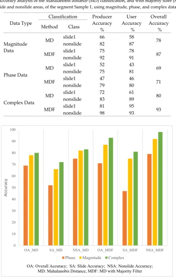
Table 3. Accuracy analysis of the Mahalanobis distance (MD) classification, and with majority filter (MDF) for slide and nonslide areas, of the segment Sample 1, using magnitude, phase, and complex data.

Data Type

Classification Producer Accuracy

%

User Accuracy

%

Overall Accuracy

% Method Class

Magnitude Data

MD slide1 66 58 78

nonslide 82 87

MDF slide1 75 78 87

nonslide 92 91

Phase Data

MD slide1 52 43 69

nonslide 75 81

MDF slide1 47 46 71

nonslide 79 80

Complex Data

MD slide1 72 61 80

nonslide 83 89

MDF slide1 81 95 93

nonslide 98 93

Figure 4. Accuracy comparison of the Mahalanobis distance classification and with majority filter, of the segment Sample 1, for the phase, magnitude, and complex data.

0 10 20 30 40 50 60 70 80 90 100

OA_MD SA_MD NSA_MD OA_MDF SA_MDF NSA_MDF

Accuracy

Phase Magnitude Complex

(8)

Figure 5. Complex data classification for the segment Sample 2: (a) without majority filter; (b) with majority filter; (c) optical image overlaid with slide and nonslide class shapes.

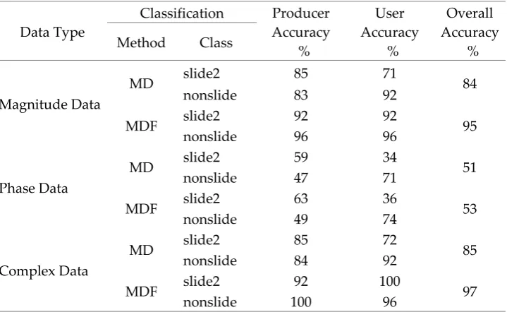
Table 4. Accuracy analysis of the Mahalanobis distance (MD) classification, and with majority filter (MDF) for slide and nonslide areas, of the segment Sample 2, using magnitude, phase, and complex data.

Data Type

%

User Accuracy

%

Overall Accuracy

% Method Class

Magnitude Data

MD slide2 85 71 84

nonslide 83 92

MDF slide2 92 92 95

nonslide 96 96

Phase Data

MD slide2 59 34 51

nonslide 47 71

MDF slide2 63 36 53

nonslide 49 74

Complex Data

MD slide2 85 72 85

nonslide 84 92

MDF slide2 92 100 97

(9)

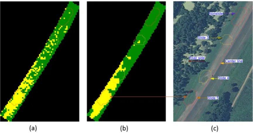
Sample 3 included, in addition to the one active slide, 2 slides (numbered 3 and 4) which had been repaired by the time of image acquisition. Many of the false positive pixels fall in this area. Because these slide areas were repaired only two months prior to the time of image acquisition, they still have characteristics more similar to the active slide than the “healthy” areas, in terms of surface roughness and differences in the grass cover. These characteristics likely influenced the classification.

Figure 7. Complex data classification for the segment Sample 3: (a) without majority filter; (b) with majority filter; (c) optical image overlaid with slide and nonslide class shapes.

0 10 20 30 40 50 60 70 80 90 100

Accuracy

(10)

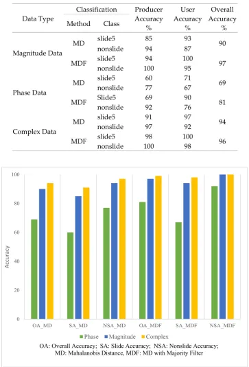
Table 5. Accuracy analysis of the Mahalanobis distance (MD) classification and with majority filter (MDF) for slide and nonslide areas, of the segment Sample 3, using magnitude, phase, and complex data.

Data Type

%

User Accuracy

%

Overall Accuracy

% Method Class

Magnitude Data

MD slide5 85 93 90

nonslide 94 87

nonslide 100 95

Phase Data

MD slide5 60 71 69

nonslide 77 67

MDF Slide5 69 90 81

nonslide 92 76

Complex Data

MD slide5 91 97 94

nonslide 97 92

nonslide 100 98

5. Conclusions

A supervised classification method based on the Mahalanobis distance for levee slide detection using complex SAR imagery is presented. In addition, we have implemented a majority filter as a post-processing step in order to improve the accuracy. The effectiveness of the algorithms is demonstrated using fully quad-polarimetric L-band SAR imagery from the NASA JPL’s UAVSAR. The cross-polarized products, HHHV, HHVV, and HVVV, are used based on the assumption that

0 20 40 60 80 100

Accuracy

(11)

they carry more information about the surface scattering properties. The study area is a section of the lower Mississippi River valley in the southern USA. The classification results obtained for all three cases (magnitude, phase, and full complex data), with accuracies for the complex data being higher, indicate that the use of polarimetric SAR can effectively detect slump slides on earthen levees. In addition to the active slide areas, other anomalous areas are also detected. Some of these are previous slide areas that had been repaired just two months prior to the time of image acquisition and still appear similar enough to the active slide to be detected by the classification technique. Furthermore, although the test study area is small, including only one active slide area for each segment, the methodology presented in this paper shows promising results. Planned future work includes the use of larger test areas consisting of more active slides, seasonal images acquired by the SAR, and different geometrical orientations of the levee.

Acknowledgments: This work was supported by the National Science Foundation grant number: OISE-1243539, and by the NASA Applied Sciences Division under grant number: NNX09AV25G. The authors would like to thank the US Army Corps of Engineers, Engineer Research and Development Center and Vicksburg Levee District for providing ground truth data and expertise; NASA Jet Propulsion Laboratory for providing the UAVSAR image; and GRI levee team.

Author Contributions: Ramakalavathi Marapareddy implemented the classification methods on image processing tools. James V. Aanstoos supervised the work, provided imagery and data and was the principal investigator for the project. Nicolas H. Younan supervised and provided guidance. Ramakalavathi Marapareddy, James V. Aanstoos, and Nicolas H. Younan analyzed the results and wrote the paper.

Conflicts of Interest: The authors declare no conflict of interest.

References

1. Aanstoos, J. V.; Hasan, K.; O’Hara, C.G.; Prasad, S.; Dabbiru, L.; Mahrooghy, M.; Nobrega, R.; Lee, M.L.; Shrestha, B. Use of Remote Sensing to Screen Earthen Levees. In Proceedings of the 39th Applied Imagery Pattern Recognition Workshop (AIPR), Washington, DC, USA, 13–15 October 2010; pp. 1–6.

2. Dunbar, J.;USACES’s Lower Mississippi Valley Engineering Geology and Geomorphology Mapping Program for Levees, presentation at the Vicksburg, MS, USA, 16 April 2009.

3. Hossain, A.K.M.A.; Easson, G.; Hasan, K. Detection of Levee Slides Using Commercially Available Remotely Sensed Data. Environ. Eng. Geosci. 2006, 12, 235–246.

4. Lin, S. W.; Ying, K.C.; Chen, S.C.; Lee, Z. J. Particle swarm optimization for parameter determination and feature selection of support vector machines. Expert Sys. Appls. An Int. J. 2008, 35(4), 1817-1824. 5. Ince, T.; Kiranyaz, S.; Gabbouj, M. Classification of Polarimetric SAR Images Using Evolutionary RBF

Networks. 20th_{Int. Conf. Pattern Recognition 2010, 4324-4327.}

6. Alvarez-Perez, J. L. Coherence, Polarization, and Statistical Independence in Cloude-Pottier’s Radar Polarimetry. IEEE Trans. Geosci. Remote Sens. 2011, 49(1-2), 426-441.

7. Han, Y.; Shao, Y. Full Polarimetric SAR Classification Based on Yamaguchi Decomposition Model and Scattering Parameters. Progress in Informatics and Computing. IEEE Int. 2010, 2, 1104-1108.

8. Jong-Sen, L.; Pottier, E. Polarimetric radar imaging: from basics to applications. CRC Press, Taylor & Francis Group. 1st _{Ed. 2009, ISBN-13: 978-1420054972.}

9. Kong, J. A.; Schwartz, A. A.; Yueh, H. A.; Novak, L.M.; Shin, R.T. Identification of terrain cover using the optimal polarimetric classifier. J. Electromagnet. Waves Applicat. 1988, 2(2), 171-194.

10. Lee, J. S.; Grunes, M. R. Classification of multi-look polarimetric SAR imagery based on complex Wishart distribution. Int. J. Remote Sens. 1994, 15(11), 2299-2311.

11. Lee, J. S.; Grunes, M.R.; Anisoworth, T.L.; Du, L.J.; Schuler, D.L.; Coulde, S.R. Unsupervised classification using polarimetric decomposition and the complex Whishart classifier. IEEE Trans. Geosci. Remote Sens.

1999, 35, 2249–2258.

12. Cloude, S. R.; Pottier, E. An entropy based classification scheme for land applications of polarimetric SAR.

IEEE Trans. Geosci. Remote Sens. 1997, 35, 68–78.

(12)

14. Aanstoos, J. V.; Hasan, K.; O’Hara, C.; Dabbiru, L.; Mahrooghy, M.; Nobrega, R.A.A.; Lee, M.M. Detection of Slump Slides on Earthen Levees Using Polarimetric SAR Imagery. In Proceedings of the Conference: 2012 IEEE Applied Imagery Pattern Recognition Workshop, Washington, D.C., U.S.A, 9–11 October 2012.

15. ENVI version 5.1. Exelis visual information solutions user guides and tutorials. http://www.exelisvis.com/Learn/Resources/Tutorials.aspx, (accessed Nov. 2014)

16. Richards, J. A. Remote Sensing Digital Image Analysis 1999, Springer-Verlag, Berlin, 240.

17. Al-Ahmadi, F. S.; Hames, A. S. Comparison of Four Classification Methods to Extract Land Use and Land Cover from Raw Satellite Images for Some Remote Arid Areas, Kingdom of Saudi Arabia. Earth Sci. 2009, 20 (1), 167-191.

18. Morton, J. C. Image Analysis, Classification and Change Detection in Remote Sensing: With Algorithms for ENVI/IDL and Python 2014, 3rd_{Ed. CRC Press. 1-576}