Developing of a thermodynamic model for the performance analysis of a Stirling engine prototype
Miguel Torres García*, Elisa Carvajal Trujillo, José Antonio Vélez Godiño, David Sánchez
Martínez
University of Seville-Thermal Power Group - GMTS Escuela Técnica Superior de Ingenieros Industriales
Camino de los descubrimientos s/n 41092 SEVILLA (SPAIN) e-mail: [email protected]
KEYWORDS
Stirling engine, combustion model
Abstrac
The scope of the study developed by the authors consists in comparing the results of simulations generated from different thermodynamic models of Stirling engines, characterizing both instantaneous and indicated operative parameters. The elaboration of this study aims to develop a tool to guide the decision-making process regarding the optimization of both performance and reliability of developing Stirling engines, such as the 3 kW GENOA 03 unit, on which this work focuses. Initially, the authors proceed to characterize the behaviour of the aforementioned engine using two different approaches: firstly, an ideal isothermal model is used, the simplest of those available; proceeding later to the analysis by means of an ideal adiabatic model, more complex than the first one. Since some of the results obtained with the referred ideal models are far from the expected actual ones, particularly in terms of thermal efficiency, the authors propose a set of modifications to the ideal adiabatic model. These modifications, mainly related to both heat transfer and fluid friction phenomena, are intended to overcome the limitations derived from the idealization of the engine working cycle and are expected to generate results closer to the actual behaviour of the Stirling engine, despite the increase in the complexity related to the modelling and simulation processes derived from those.
1. INTRODUCTION
The increase of thermal efficiency, jointly with the reduction of pollutant emissions, is the most significant challenge faced by the combustion engine industry, as a consequence of the increasingly demanding legislation in force in most of the industrialized countries [1]. The aforementioned demand originates relevant necessities of developing continuous improvement methods within the combustion engine sector. Although different difficulties
still need to be addressed, the Stirling engine is currently one of the most promising options among the strategies considered by the combustion engine sector as an alternative to the conventional internal combustion units. From the thermodynamic point of view, Stirling units consist of closed-cycle regenerative thermal engines with a gaseous working fluid and external heat supply, whose operation is based on the cyclic compression and expansion of the mentioned gas at two different temperature levels. The main features of the Stirling engine include high efficiency, mechanical simplicity, low vibration and noise levels and the attractive possibility of using a wide range of heat sources. On the other hand, Stirling engines are also characterized by a low output power-to-weight ratio, slow load ramps and difficult sealing when using low molecular weight substances.
A diverse range of practical applications and a significant number of theoretical studies have been proposed since the beginning of the 19th century, when Robert Stirling designed a thermal engine aimed at competing the steam engine. Unfortunately, such applications have rarely gone beyond the academic or experimental level. However, the newly proposed use of Stirling engines combined with the harnessing of heat from renewable sources currently constitutes a promising line of research, due to the attractive combination of extraordinary levels of both versatility and efficiency [2-4].
Although different contributions have been made during the last decades regarding the performance of Stirling engines, one of the most relevant works was developed by Senft [5-9], who intensively analysed the performance of Stirling engines using different mechanical models. After comparing different typologies of reciprocating engines, the aforementioned author concluded that maximum thermal efficiency was achieved by Stirling engines.
Other noteworthy contributions regarding the analysis of the performance of Stirling engines are those derived from the finite-time thermodynamics [10-22], theory initially proposed by Andresen et al [23].
Power, efficiency, performance, ecological aspects and entropy generation of both traditional and solar-driven Stirling engines coupled to infinite or finite heat-capacity reservoirs with general working medium and quantum working medium were optimized.
Regarding the heat transfer, a key issue further addressed in this paper, different researchers [24–25] have proven the significant influence of the heat transfer laws used in the models over the optimal performance of Stirling engines, mainly due to the irreversibilities derived from that. Additionally, regarding the heat transfer topic in Stirling engines, it is noteworthy the contributions made by Hsieh et al. [21] and, again, by Senft [22,23]. The latter proposed an irreversible model based on the finite-time thermodynamics approach to study the performance of Stirling engines, considering a model including mechanical losses, heat capacities and, finally, heat losses, which were modelled in accordance with a Newtonian heat transfer law.
developed by means of further presented numeric models, all of them developed in Matlab ® tool code [26]. The referred models are used to analyse the engine performance and to compare it with the actually expected behaviour. Additionally, these simulations allow the study of the operative conditions present in the different components involved in the unit operation.
Also the present project makes an analysis on a Stirling commercial model GENOA 03 engine (GenoaStirling s.r.l.) [27] for electric power generation, of 3 KW of nominal power that uses pressurized air as a working fluid. A unit of this engine has been transferred by the University of Genoa to the University of Seville for its experimental analysis. The two following sections are structured to describe the main features, the governing equations, the simulation algorithm and the most relevant results related to the two ideal thermodynamic models used by the authors: the ideal isothermal model and the ideal adiabatic model. Afterwards, a set of modifications to the ideal adiabatic model are proposed, modifying the heat transfer assumptions and incorporating frictional losses to the mass flows. As previously mentioned, the purpose of these modifications is to simulate the engine behaviour with higher accuracy, allowing also the analysis of different components performance, such as the regenerator or the cooler, being both key components of the Stirling engine in terms of efficiency. Finally, the authors compare the main results obtained using the mentioned different approaches.
2. ENGINE DATA TECHNICAL
Fig. 1. Genoa Stirling engine scheme [27].
3. NUMERICAL MODEL
In the following paragraphs, numerical models will be developed to evaluate the operating conditions of the engine. By the order of complexity and approximation to real behaviour, they have been: the ideal isothermal model, the ideal adiabatic model and the real adiabatic model.
In addition to these models, another model based on the adiabatic model has been developed, which considers the heat transfer and the load losses in the exchangers of the engine. This model is called a simple adiabatic model.
3.1. Ideal isothermal model
It is based on the model developed by Schmidt, who was the first to thermodynamically model the Stirling cycle. The behaviour of the working fluid in the compression and expansion cylinders is considered isothermal, which eliminates the complexity associated with the temperature variations in those cylinders.
The main hypotheses of this model are the following:
• The pressure has the same value in any component of the motor for the same moment of time, that is, the missing loads are neglected.
• The mass of the working fluid is constant, that is to say, the gas leaks out of the engine are negligible.
• The behaviour of the working fluid is considered according to an ideal gas.
• The speed is constant.
• It is considered a permanent cyclic system, that is to say, there are no dynamic variations between one cycle and the next one.
• Variations in kinetic and potential energy are neglected.
• The volume variations in the engine workspaces are sinusoidal.
The advantages offered by this model are several. Firstly, considerations such as the sinusoidal volume variation simplify the formulation of the equations to algebraic relationships, making their calculation analytically workable, long before the computer age. Secondly, the indicated work calculated from the P-V diagram is quite accurate.
However, Schmidt's analysis is not able to accurately determine the heat fluxes throughout the cycle, which affect efficiency. That is why the efficiency calculated with this pattern coincides with the efficiency of Carnot. This is due to the fact that it is considered that the compression and expansion spaces are isothermal and exchangers are as ideals, so the model has maximum efficiency. Taking into account these considerations, the temperatures of each component of the model is represented in Figure 2.
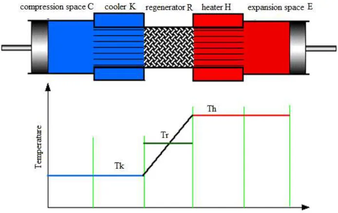
Figure 2 Isothermal model and temperature distribution.
The subscript represents the component to which it refers to: compression cylinder "C", cooler "K", regenerator "R", heater "H" and expansion cylinder "E".
3.2. Ideal isothermal model equations.
The conservation equations of mass and energy are considered in this pattern. Its variation is considered with the crank angle. The total mass of the system M is the sum of all component masses m and it is considered constant over time and with the crank angle, Eq 1:
𝑀 = 𝑚 + 𝑚 + 𝑚 + 𝑚 + 𝑚 (1)
Since the behaviour of the gas is considered ideal, the total mass is defined by Eq 2.
𝑚 =𝑝 ∙ 𝑉
𝑅 ∙ 𝑇 ⟶ 𝑀 = 𝑝 𝑅∙
𝑉
𝑇 +
𝑉
𝑇 +
𝑉
𝑇 +
𝑉
𝑇 +
𝑉 𝑇
(2)
The effective temperature in the regenerator is necessary, and it is calculated as the logarithmic average of the temperatures in cooler and heater, Eq 3.
𝑇 = (𝑇 − 𝑇 ) ln 𝑇 𝑇
Taking into account the volume variations Vc and Vees. to isolate the pressure p as a function of these volume variations is possible, Eq 4.
𝑝 = 𝑉 𝑀 ∙ 𝑅
𝑇 +
𝑉
𝑇 +
𝑉
𝑇 +
𝑉
𝑇 +
𝑉 𝑇
(4)
Therefore, the work done by the system in a complete cycle is expressed by the cyclic integral of pdV, Eq 5:
𝑊 = 𝑊 + 𝑊 = 𝑝𝑑𝑉 + 𝑝𝑑𝑉 = 𝑝 𝑑𝑉
𝑑𝜃 + 𝑑𝑉
𝑑𝜃 𝑑𝜃
(5)
Volumes Vc and Ve vary over the course of the time depending on the position of the piston in the cylinder. In an alpha-type configuration, the phase angle between the expansion and compression volume variations is α = π / 2. In the Eq. 6. is represented the compression and expansion cylinder Volume variation with crank angle, where Vm is the clearance volume of each cylinder, Acyl is the cylinder area, d is the bore, r is the crank and l is the connecting rod length, Figure 3.
𝑉 (𝜃) = 𝑉 , + 𝑥(𝜃) ∙ 𝐴 =
= 𝑉 , + 𝑟 + 𝑙 − 𝑟 ∙ cos(𝜃) + 𝑙 ∙ cos 𝑎𝑟𝑠𝑒𝑛 𝑟
𝑙 ∙ sin(𝜃) ∙ 𝜋 ∙ 𝑑
4
𝑉 (𝜃) = 𝑉 , + 𝑥(𝜃) ∙ 𝐴 =
= 𝑉 , + 𝑟 + 𝑙 − 𝑟 ∙ cos 𝜃 −
𝜋
2 + 𝑙 ∙ cos 𝑎𝑟𝑠𝑖𝑛 𝑟
𝑙 ∙ sin 𝜃 − 𝜋 2
∙ 𝜋 ∙ 𝑑 4
Fig. 3. Piston - connecting rod - crankshaft mechanism.
As well as the total mass of the system, the total volume of the system is the sum of the volumes of each component, Eq 7 is finally equivalent to:
𝑉 = 𝑉 + 𝑉 + 𝑉 + 𝑉 + 𝑉 (7)
Since the volumes Vc and Ve vary with the crankshaft angle, the total volume of the system and the pressure in the engine also vary with this angle, for what this angle is the only variable independent of the set of equations.
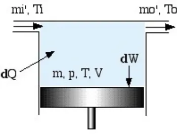
The first principle of thermodynamics is applied to each component of the engine. Taking into account the ideal isothermal model in terms of energy flow, the energy equation for a generic engine cell has arisen, which can be indifferently a heat exchange cell, or work, in which in addition to the energy exchange with the outside , there is a mass flow of input and output, Figure 4.
Fig. 4: Generic cell diagram of the motor.
The enthalpy in the particular cell is provided by the difference between mass flow and inlet temperatures (mi and Ti) and output (mo and To) while the heat or work flows are represented by dQ and dW respectively (figure 4). In this way the energy balance remains in the expression: "Heat supply + net enthalpy = work in the cell + increase of internal energy."
For an ideal gas, enthalpy and internal energy depend only on the temperature, then specific enthalpy and specific internal energy can be expressed as ℎ = 𝑐 𝑇 and 𝑢 = 𝑐 𝑇, resepctively. Then the energy balance [28] is represented by Eq. 8:
𝑑𝑄 + 𝑐 𝑇 𝑚′ − 𝑐 𝑇 𝑚′ = 𝑑𝑊 + 𝑐 𝑑(𝑚𝑇) (8)
𝑑𝑄 + 𝑐 𝑇𝑑𝑚 = 𝑑𝑊 + 𝑐 𝑇𝑑𝑚 (8)
Assuming ideal gas, the gas constant is R = Cp-Cv. Then, the energy balance is represented by Eq 9:
𝑑𝑄 = 𝑑𝑊 − 𝑅𝑇𝑑𝑚 (9)
Finally, the heat transferred to the gas during the cycle is obtained from the integration of dQ. However, the hypothesis of permanent cyclical system implies a cyclical variation of the null mass throughout the cycle, for all the cells. By integrating, the following is obtained:
𝑄 = 𝑊 𝑄 = 𝑊 𝑄 = 0 𝑄 = 0 𝑄 = 0
The above considerations lead to these results:
• The heat transferred or absorbed by the gas is entirely turned into work in the compression and expansion spaces.
• The net heat rate of the regenerator is zero, this is due the regenerator is ideal.
• There is no heat transfer between the gas and the environment in the heater or cooler.
The last consideration makes the hot and cold exchangers seemingly useless pieces in this model, since the supply and transfer of heat occurs in the spaces of expansion and compression. This contradiction is a direct consequence of the hypothesis of the isothermal model of maintaining expansion and compression spaces at the same temperature as their associated heat exchangers (heater and cooler respectively), which is by all accounts an incorrect assumption.
In real machines, the ideal case tends to consider the spaces where gas energy is transformed into work, as adiabatic domains, and not isothermal, which implies that the net heat of the cycle must be provided by the exchangers.
3.4 Characterization of the engine in the model
The model is particularized to the GENOA 03 engine. The steps taken to adapt the isothermal model to the geometry and operating conditions of the engine are described below. This numerical model has been implemented using the Matlab ® software.
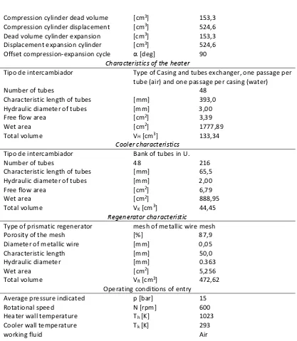
On the table 1, all the geometric characteristics of the GENOA 03 engine are exposed for its implementation in a mathematical model.
Connecting rod length l [mm] 210,0
Rotation radius of connecting rod r r [mm] 30
Diameter of the cylinder d [mm] 110,0
Compression cylinder dead volume [cm3] 153,3
Compression cylinder displacement [cm3] 524,6
Dead volume cylinder expansion [cm3] 153,3
Displacement expansion cylinder [cm3] 524,6
Offset compression-expansion cycle [deg] 90 Characteristics of the heater
Tipo de intercambiador Type of Casing and tubes exchanger, one passage per tube (air) and one passage per casing (water)
Number of tubes 48
Characteristic length of tubes [mm] 393,0
Hydraulic diameter of tubes [mm] 3,00
Free flow area [cm2] 3,39
Wet area [cm2] 1777,89
Total volume VH [cm3] 133,34
Cooler characteristics Tipo de intercambiador Bank of tubes in U.
Number of tubes 48 216
Characteristic length of tubes [mm] 65,5
Hydraulic diameter of tubes [mm] 2,00
Free flow area [cm2] 6,79
Wet area [cm2] 888,95
Total volume VK [cm3] 44,45
Regenerator characteristic
Type of prismatic regenerator mesh of metallic wire mesh
Porosity of the mesh [%] 87,9
Diameter of metallic wire [mm] 0,05
Characteristic length [mm] 50,0
Hydraulic diameter [mm] 0.363
Wet area [cm2] 5,256
Total volume VR [cm3] 472,62
Operating conditions of entry
Average pressure indicated p [bar] 15
Rotational speed N [rpm] 600
Heater wall temperature Th [K] 1023
Cooler wall temperature Tk [K] 293
working fluid Air
Table 1 Geometric characteristics of the GENOA 03 engine.
cooler and the compression cylinder, which have been unappreciated in the isothermal model to simplify the calculations. However, these interconnection volumes are reflected in the models of the following sections.
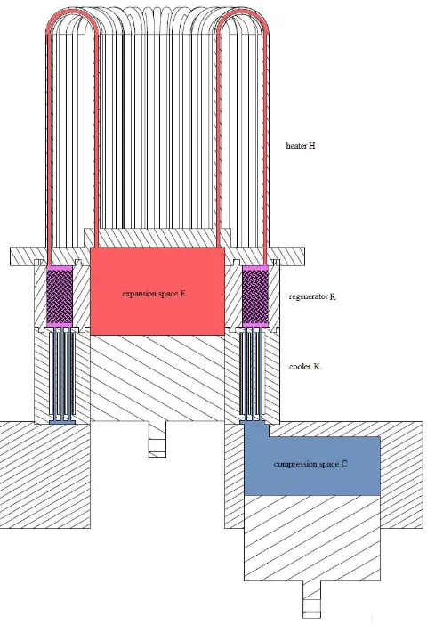
Fig. 4: View of the middle section of the engine component set.
3.5 Numerical simulation and results.
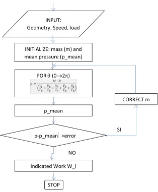
Once the engine is geometrically characterized and its boundary conditions defined, the isothermal model is simple to implement. Noting the flow diagram of Figure 5, the model incorporates a total mass of the initial engine m, and an effective average pressure p. Then the code calculates the total average pressure for each value of θ as a function of the initialized mass (p mean) and it compares it with the reference pressure. If the difference between the two is greater than the manageable error, the code enters the iteration loop correcting the mass, until the convergence. Then the indicated work of the cycle can be obtained.
Fig. 5: Flow diagram of the isothermal model
A total mass value of air is obtained from the simulation, once the convergence criteria is reached, being:
𝑀 = 0,00144 [𝑘𝑔]
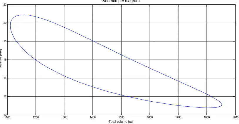
Finally, Figure 6 represents the instantaneous pressure versus volume: INPUT:
Geometry, Speed, load
INITIALIZE: mass (m) and mean pressure (p_mean)
FOR (02)
p_mean
p-p_mean>error
Indicated Work W_i
CORRECT m
NO
SI
Fig. 6: P-V diagram of the isothermal model.
The indicated work of the cycle is obtained by integrating the area of this P-V diagram. Other interesting results from the GENOA 03 simulation are shown following:
𝑄 = 389,6 [𝐽] 𝑄 = −111,6 [𝐽]
𝑊 = 278,0 [𝐽] 𝜂 = 0,714
As expected, the performance matches the ideal value of Carnot. Since the work and the speed are known, the indicated power of the cycle for boht cylinders are calculated as Eq , knowing the work, and the system of rotation is defined as:
𝑃 = c ·𝑊 ∙ 𝑁
60 = 5,560 [𝑘𝑊]
(9)
4. The ideal adiabatic model (Urieli).
This model is based on the work of Dr. Israel Urieli[29], who developed the adiabatic analysis for the Stirling engine as part of his doctoral thesis, and Theodor Finkelstein, who defined for the first time models of adiabatic work spaces in the engines of air. The adiabatic analysis is similar in its approach to the Schmidt model, with the main exception that it is considered that the working fluid in the compression and expansion cylinders undergo an adiabatic process instead of isothermal.
1100 1200 1300 1400 1500 1600 1700 1800 1900
10 12 14 16 18 20 22
Total volume [cc]
P
re
ss
u
re
[b
ar
]
Therefore, an ideal adiabatic model represents the maximum efficiency. In addition, to high performance engines this value is quite similar to the real efficiency value. Therefore, it is considered that an analysis of a Stirling engine must reach at least the adiabatic model to believe that the results of the simulations are useful in such analysis.
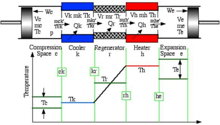
Regarding the isothermal model, the rest of the hypotheses and considerations are maintained, as well as the simplification of the engine in five components in series, nevertheless there are certain variables that must be added to the original formulation concerning to the heat exchangers in the adiabatic model, as can be seen in the schematic form of the model (Figure 6).
Fig. 7. Schematic model and temperature chart of the adiabatic model.
It is necessary to include the four interfaces associated with the five components of the engine in this model, since now the temperature between the workspaces and the exchangers are not constant in a cycle, as it was the case of the isothermal model. Each interface is distinguished according to the following sub-indices; ck, between the compression cylinder and the cooler, kr, between cooler and regenerator, rh, between regenerator and heater, and finally between the heater and the expansion cylinder. For example, mCK 'represents the mass flow between the compression cylinder and the cooler.
implies the displacement from the compression space in the direction of expansion and vice versa. Such a condition is signified in the algorithm as:
If mck' > 0 then Tck = Tc else Tck = Tk If mhe' > 0 then The = Thelse The = Te
In summary, the hypotheses and simplifications carried out by Urieli and Finkelstein were:
• The compression and expansion spaces are adiabatic. (The heat exchanged between the cylinders and the environment is zero).
• Gas leaks into the environment are negligible.
• The pressure in an instant of time is the same throughout the entire engine. Losses of load are not considered.
• The movement of the piston-connecting rod-crankshaft chain follows the sinusoidal law described in the isothermal model (Figure 3).
• The heat transfer in the exchangers is considered good enough to maintain the temperatures TK and TH and the volume VK and VH of the gas, constant in its wake through the cooler and heater, respectively.
• The performance of the regenerator is assumed to be good enough to maintain a linear distribution of temperatures along its length, with the temperature TK for the face in contact with the cooler and TH for the side of the heater.
4.1 Development of the equations.
The set of equations of the model is based on the solution of the differential of pressure and the differential of mass per element that takes place for an increase of the angle of rotation of the crankshaft. In this way, the differential shape of mass conservation, amount of movement and conservation of energy in expansion and compression spaces are used. In addition to the state equations applied to the exchangers.
Firstly, the differential way of conservation of the mass is as following (Eq. 10)leads us to:
Similarly to the isothermal model, the behaviour of the gas is considered as ideal gas. This hypothesis is close to the real behaviour since the gas is to be found in far away conditions to the critical point.
In this way, deriving the form of the law of ideal gases for pressures, and knowing that throughout the cycle the temperatures and volumes in the exchangers are constant, we obtain (Eq. 11):
𝑝 = 𝑀𝑅 𝑉 𝑇 + 𝑉 𝑇 + 𝑉 𝑇 + 𝑉 𝑇 + 𝑉 𝑇 → 𝑑𝑚 𝑚 , , =𝑑𝑝 𝑝 , , (11)
Eq. 12 is obtained by substituting in the differential form of conservation of mass the equation of state:
𝑑𝑚 + 𝑑𝑚 + 𝑑𝑝 𝑚
𝑝 +
𝑚
𝑝 +
𝑚
𝑝 = 0
→ 𝑑𝑚 + 𝑑𝑚 +𝑑𝑝 𝑅 𝑉 𝑇 + 𝑉 𝑇 + 𝑉 𝑇 = 0
(12)
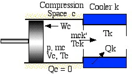
The intended objective in the isothermal formulation is to obtain a relationship for the pressure differential depending only on the independent variable, in this case the angle θ. Then it is necessary to clear the terms of dmC and dmE. Figure 7 is a diagram of the variables and flows in the compression cylinder. Applying the energy balance to this control volume, Eq. 13 is obtained.
Figure 7. Adiabatic diagram of the compression cylinder and cooler.
The compression is adiabatic, then dQc = 0, and the work is defined by, dWc = pdVc. On the other hand, the differential mass dmc is equal to the mass flow through the interface CK, mck, reducing the equation to Eq. 14:
𝑐 𝑇 𝑑𝑚 = 𝑝𝑑𝑉 + 𝑐 𝑑(𝑚 𝑇 ) (14)
By substituting the equation of state, and ideal gas relations, an expression of the differential mass as a function of pressure is obtained. This relationship can be expressed, Eq. 15 analogously for both the compression space and the expansion space, obtaining:
𝑑𝑚 =𝑝𝑑𝑉 + 𝑉 𝑑𝑝 𝛾 𝑅𝑇 𝑑𝑚 = 𝑝𝑑𝑉 +𝑉 𝑑𝑝 𝛾 𝑅𝑇 (15)
Finally, the differential pressure for each instant of the cycle is defined by Eq. 16:
−𝛾𝑝 𝑑𝑉𝑇 + 𝑑𝑉𝑇 𝑉 𝑇 + 𝛾 𝑉 𝑇 + 𝑉 𝑇 + 𝑉 𝑇 + 𝑉 𝑇 (16)
The equations associated with dp and dm pose a system of differential equations with several unknowns associated with the temperatures Tc and Te and the masses mc and me. Given that the resulting system is non-linear, it can only be solved by numerical integration, as a problem of initial values associated with an iterative process defined by certain convergence parameters.
Once p and m have been evaluated, the rest of the variables can be obtained through mass balance and state equations. The parameters dVc, dVe, Vc and Ve are easily calculated by the kinematics relations. The differential equations of the temperature in the workspaces derive from the ideal gas equation, Eq. 17:
𝑑𝑇 = 𝑇 𝑑𝑝 𝑝 + 𝑑𝑉 𝑉 + 𝑑𝑚 𝑚 𝑑𝑇 = 𝑇 𝑑𝑝 𝑝 + 𝑑𝑉 𝑉 + 𝑑𝑚 𝑚 (17)
The indicated work of the cycle is the sum of the work done by each cylinder, Eq. 18:
𝑑𝑊 = 𝑑𝑊 + 𝑑𝑊 = 𝑝𝑑𝑉 + 𝑝𝑑𝑉 (18)
Through the equation of the energy, and replacing the values of dT and dW, a more adequate form of that equation is obtained, Eq. 19, easily applicable to each component.
𝑑𝑄 + 𝑐 𝑇 𝑚 − 𝑐 𝑇 𝑚 = 𝑐 𝑝𝑑𝑉 + 𝑐 𝑉𝑑𝑝 𝑅
For example, for the three exchangers, where there is no work exchange and the volume is constant, Eq. 20 is obtained by reducing the previous expression:
𝑑𝑄 =𝑐 𝑉 𝑑𝑝
𝑅 − 𝑐 (𝑇 𝑚 − 𝑇 𝑚 )
𝑑𝑄 =𝑐 𝑉 𝑑𝑝
𝑅 − 𝑐 (𝑇 𝑚 − 𝑇 𝑚 )
𝑑𝑄 =𝑐 𝑉 𝑑𝑝
𝑅 − 𝑐 (𝑇 𝑚 − 𝑇 𝑚 )
(20)
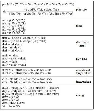
The final system of differential equations and algebraic relationships which are necessary for the numerical solution of the ideal adiabatic model is summarized in table 2.
Table 2. Set of equations of the ideal adiabatic model.
Once the system of necessary equations is stablished, and having characterized the motor in the development of the isothermal model, the objective is now to solve the differential equations of temperature, mass and pressure in both cylinders, to represent the distribution of these parameters in a complete cycle, and calculate the performance of the engine.
In this case, the problem is of a non-linear nature much more discontinuous than in the isothermal case, since two temperatures have been incorporated conditional to the direction of flow.
Figure 8 shows the simplified flow diagram of the ideal adiabatic model and tries to express in a simplified way the execution order of the solution algorithm, although some key operations are missing, such as the one related to the conditional temperatures.
Figure 8. Simplified flow chart of the ideal adiabatic model.
variables is known, and the equations are integrated throughout the cycle, that is to say, the crankshaft makes one full circle. However, the adiabatic model corresponds more like a problem of boundary conditions and not of initial values, since these values are not known in advance.
Although if we assign initial values from the solution of the isothermal model, it is possible to integrate the equations from these values. After several iterations of the complete cycle, the condition that establishes that the values of the variables at the end of the cycle (2π) and at the beginning of the cycle (0) coincide, which is nothing but the condition of reaching the permanent cyclical system of the cycle.
Once the convergence in the previous condition is obtained, the next step is to satisfy the operating conditions, in such a way that the average pressure of the cycle coincides with the design pressure, for this purpose a loop of iteration is required.
With all the considerations set out above, the algorithm is stable enough to generate the convergence of the solution by changing parameters such as the motor geometry or the operating conditions of the motor, in a range close to the design point.
4.3 Numerical simulation and results.
Once the solution for the adiabatic model is obtained, it is interesting to show the temperature distribution, where now Te and Tc are variable with time, as well as the distribution of energy flows through each component. In Figure 9 is represented the temperature distribution of the adiabatic model, the compression and expansion temperatures can be observed to be variable throughout the cycle.
The most striking is that this temperature variation implies a reduction in the average temperature in the expansion cylinder, since the oscillation has an amplitude of around 200K, this decrease in temperature with respect to the adiabatic model, will be reflected in the thermal performance of the machine, which will no longer be equivalent to the ideal performance of Carnot, yielding a much more realistic ideal value.
Regarding the energy flows along the motor, in Figure 10 the values relative to the heat flow in the exchangers next to the values of the net work, appears overlapping. This diagram gives very valuable information of the behaviour of the ideal adiabatic model. It is worth mentioning that the integral of the curve does not correspond to the net value of each parameter, but also the value for each point of the curve is the accumulated net value, being zero at the beginning of the cycle, (reference), and being the net value for a complete cycle at the point θ = 360 °. With regard to work, those associated with the compression and expansion spaces appear, and the net work, which is the sum of both values; being the net work of expansion: positive, and that of compression: negative.
The heat flow of the regenerator is zero at the end of the cycle, since we consider it ideal in this model. However, throughout the cycle, energy values of the order of ten times the final net work are produced, which implies that the regenerator is a key element in the design of the engine, since the performance of this one in a non-ideal case, depends crucially on the capacity of such a component to absorb and yield large heat flows.
Figure 10. Distribution of net energy flows of the adiabatic model.
To illustrate qualitatively these net flows of heat and work, they are well represented in the right margin of Figure 10.
Figure 11. Pressure diagrams of isothermal and adiabatic cycle volume.
By integrating the area of the P-V diagram of figure 11 for the adiabatic model, the indicated work of the cycle is finally obtained. And the other equations, the heat fluxes, and the thermal efficiency of the GENOA 03 engine:
𝑄 = 449,8 [𝐽] 𝑄 = −176,2 [𝐽]
𝑊 = 274,1 [𝐽] 𝜂 = 0,61
The power, calculated in the same way as in the case of the isothermal model, is therefore, Eq. 21:
𝑃 = c ·𝑊 ∙ 𝑁
60 = 5,482 [𝑘𝑊]
(21)
By means of conclusions for this section, you can say that the adiabatic model is more realistic than the isothermal model, however, several of the results remain inconsistent with the real behaviour of an alternative engine, especially those referring to the exchangers. As a compensatory measure, the adiabatic analysis, considering all the operative parameters and variables that it is capable of resolving, offers a very valuable information to know the operative conditions of each of its components separately.
11008 1200 1300 1400 1500 1600 1700 1800 1900 10
12 14 16 18 20 22
Volume [cc]
P
re
ss
u
re
[b
ar
]
Diagrama Presión - Volumen
Adiabático
Isotermo
Adiabatic
In the case of the present project, the ideal adiabatic model has been an indispensable tool to know the mass flow of air that circulates through the exchanger, and in the directions that it makes it, and that instants of time there are spikes of flow velocity, and reversal of flow dead points, in order to design alternatives that could be compared with each other for some boundary conditions as similar to the behaviour of the real engine as possible.
In addition, the ideal adiabatic model is presented as a solid base to which you can add modifications and auxiliary functions, to make the code even more complex and cover other aspects such as the effectiveness of heat transfer in the exchangers, the effect of including the geometry of the motor with interconnections among elements, or load losses, by means of air friction on the motor walls.
The next step is to start from the adiabatic model and design a new model that is capable of evaluating changes in engine performance by modifying or changing components, such as exchangers, or more precise when it comes to defining boundary conditions, for example, define a cooling water flow at a certain temperature instead of imposing a temperature on the internal wall of the cooler.
5. The simple adiabatic model (Ohio).
The model developed below adds functions and calculation aspects complementary to the adiabatic model, from now on called the simple adiabatic model. This model keeps calling adiabatic since, although the original algorithm of the ideal model has been object of modifications, and some intermediate variables control have been added, the procedure of solution is essentially the same, and in addition, the spaces of compression and expansion walls are still considered adiabatic.
Given the fact that this model is a modification more than a numerical model properly speaking, the procedure to follow depends on the literature that is consulted, as many projects on Stirling engines, like this one, use modifications of the ideal adiabatic model.
As an example of one of these models, the approach of Urieli [29] himself will be followed. This approach adds three fundamental aspects; the heat transfer distinguishing the regenerator from the other two exchangers, and the flow friction losses in the three exchangers of the engine, and their influence on the performance of the same.
• The efficiency of the regenerator is assumed not to be ideal, if we study the influence of this parameter on the engine performance.
• The heat transfer in the cooler and heater is evaluated by means of the forced correlations convection for the transfer between the working fluid and the exchanger walls, so that a wall temperature for each exchanger is assumed.
must be provided by the indicated cycle work, by reducing the net power of the engine.
Once the model implements simultaneously the three previous aspects, the numerical simulation must be carried out for the GENOA 03 engine, and must be contrasted with the ideal models.
5.1 Characterization of the non-ideal regenerator.
As discussed on many occasions, the regenerator of a Stirling engine is a key component with a critical influence on its performance. However, throughout the history of the Stirling engine, the operation theories of this component have been based on hypotheses supported by merely experimental studies only, hardly extrapolated from a configuration or other models [30].
The regenerator is a device that works cyclically, in a direction of flow, the hot air flow from the heater, transfers part of its heat to the regenerator mesh, on the other hand, the mesh transfers as much of the heat absorbed into the cold air from the cooler as possible. In steady state therefore, the net heat transfer of the regenerator is zero.
The effectiveness of the regenerator is usually expressed as the ratio of the enthalpy variations in the real flow, with respect to the maximum theoretical variation in an ideal regenerator. However, to adapt to the simple adiabatic model, which we consider the ideal case, we define efficiency
ε
as heat transferred between the mesh and the gas in a single pass through divided by heat transferred in the regenerator of the ideal adiabatic modelFigure 12 represents the temperature evolution of both flows diagram through the regenerator, if they are no ideal.
Where we consider that the variation between temperatures, ∆T, cold and hot input and output are identical, at both ends of the regenerator. Furthermore, by observing Figure 12, the efficiency in terms of temperature can be expressed as following, Eq. 22:
𝜀 =(𝑇 − 𝑇 ) (𝑇 − 𝑇 )
(22)
Therefore, ε=1 for the ideal regenerator, while for ε=0, there is no regenerative effect. To assess the effect of these variations on cycle performance, we start from the general expression of thermal efficiency for the ideal model (with superscript '), Eq. 23.
𝜂 = 𝑊′ 𝑄′ =
(𝑄′ + 𝑄′ ) 𝑄′
(23)
Whereas, for the non-ideal case, the heat exchanged by cooler and heater is the ideal value plus the sum of the heat that the regenerator has not been able to absorb), Eq. 24:
𝑄 = 𝑄′ + 𝑄′ ( ) (24)
Substituting the values of Qh, Qk and the ideal efficiency ηi in the equation of the non-ideal thermal efficiency we obtaine the Eq. 25:
𝜂 = 𝑊
𝑄 =
(𝑄 + 𝑄 )
𝑄 =
𝜂
1 + 𝑄′ 𝑄′
( )
(25)
Knowing the thermal efficiency, nd the ratio between the heat of the regenerator and the heater in the ideal case, a proportional relationship between the efficiency of the regenerator and the non-ideal thermal efficiency can be expressed. In this way, we can observe that by varying the efficiency in its absolute range, si ε=0, the thermal efficiency falls from the ideal case ≈65% to values around 10%.
Low efficiency values, e.g. 80%, have various implications for the engine, to begin with, the overall efficiency can drop up to 30%, and furthermore, if the regenerator is not able to get rid of a considerable part of the engine, the cooler must be larger, increasing the load losses and decreasing the net work.
5.2 Characterization of heat exchangers.
temperature of the air through the exchanger, where we only consider the forced convection of the air through the tubes, and we do not consider the convective exchange with the external water or the conduction through the tube walls, as shown in the diagram in Figure 13.
Figure 13: Heat exchanger model
The efficiency of the exchangers could in advance be evaluated through the ε-NTU method (transfer units method), but to do so a more complete analysis that the one proposed by the simple model is needed. In section 5 of this project, the ε-NTU method will be implemented as a cooler analysis tool. For the present case, we start from a wall temperature Tw related to the average temperature of mass T using the convection equation, Eq. 26:
𝑄̇ = ℎ 𝐴 (𝑇 − 𝑇) (26)
Where Q' represents the heat energy, Aw refers to the "wetting area" of the exchangers and h is the convective coefficient. To evaluate this equation in terms of heat per cycle, as before, it is necessary to divide by the machine frequency, f (Hz) or (s-1), In this way we express the values of Qk and Qh as is shown in Eq. 27:
𝑄 − 𝑄, =
ℎ 𝐴 (𝑇 − 𝑇 )
𝑓 → 𝑇 = 𝑇 − 𝑓(𝑄 − 𝑄 )/(ℎ 𝐴 )
𝑄 − 𝑄 , =
ℎ 𝐴 (𝑇 − 𝑇 )
𝑓 → 𝑇 = 𝑇 − 𝑓(𝑄 − 𝑄, )/(ℎ 𝐴 )
(27)
5.3 Characterization of load losses.
Throughout the previous models we have assumed that the pressure remained constant throughout all the components of the engine for the same instant of time. However, the passage of the flow through heat exchangers, in this case, banks of tubes, and through a mesh in the case of the regenerator, generates a huge friction of the fluid on the walls of these components, being therefore a phenomenon that is necessary to contemplate in a more advanced model like this one.
These friction losses are generally called load losses, expressed in units of pressure. They have a direct influence on the expression of the indicated cycle work, which, as stated above, depends on the integration of pressure and volume in the engine workspaces, where load losses decrease the final net work.
To quantify these losses, we proceed from the expression of the indicated work and add a term of pressure loss summation in the three exchangers, ∑∆p, at the end of the pressure at one of the engine ends, obtaining Eq. 28:
𝑊 = 𝑊 + 𝑊 = 𝑝𝑑𝑉 + (𝑝 − ΣΔ𝑝)𝑑𝑉
(28)
By moving the terms of the previous expression, you can express the initial indicated work on one side and the load losses ΔW on the other in the following way, Eq. 29:
𝑊 = 𝑝(𝑑𝑉 + 𝑑𝑉 ) + (ΣΔ𝑝)𝑑𝑉 = 𝑊 − ΔW ⋯ ΔW = Δ𝑝 𝑑𝑉
𝑑𝜃 𝑑𝜃 (29)
To characterize these pressure losses in each exchanger, following the procedure described by Kakaç [31], losses within a circular duct are influenced by the fluid velocity, the density, the roughness of the tube walls as well as their diameter and length.
Expressing the previous relationships as a dimensionless set of parameters, Eq. 30 is obtained:
𝑓 = Δ𝑝
4(𝐿/𝑑 )(𝜌𝑢 /2)≡ Φ(𝑅𝑒, 𝑑 ) (30)
Figure 14 Moody's Abacus.
For its implementation in numerical models, it is more appropriate to use numerically expressible correlations, such as Drew, Koo & McAdams [32], applicable to simple pipe geometry, Eq. 31:
𝑓 = 0.00140 + 0.125𝑅𝑒 . 4 · 10 < 𝑅𝑒 < 5 · 10
(31)
Finally, the expression of the load losses in a pipe stays as follows, Eq. 32:
Δ𝑝 = 4𝑓𝐿
𝑑 𝜌𝑢
2 [𝑃𝑎] (32)
5.4 Numerical simulation and results.
Figure 15 Temperature distribution in the simple model.
Regarding load losses, Figure 16, it is interesting to analyze two aspects. The first of these is the distribution of the load losses of each element separately:
Figure 16. Load losses of the exchangers in the Simple model.
Figure 16 shows how the heater's load losses are of the order of almost six times greater than in the regenerator. This has a simple explanation if we consider the enormous length of the heater compared to the length of the cooler or regenerator. Given that the load losses depend linearly on the length of a conduit, this result seems logical, even considering that the regenerator consists of a compacted mesh, the length in the heater is a parameter of greater weight in this case. The second aspect is to observe the difference in the pressure distribution of the compression cylinder with respect to the expansion cylinder once the losses in the code have been implemented, Figure 17. The difference between the two pressures represents the load losses.
0 50 100 150 200 250 300 350
200 300 400 500 600 700 800 900 1000 1100
Ángulo de giro [deg]
T e m p e ra tu ra [K ]
Tcomp Texp Twall,k Tk Tr Th Twall,h
0 50 100 150 200 250 300 350
-2 -1.5 -1 -0.5 0 0.5 1 1.5 2 2.5
x 104
Ángulo de giro [deg]
P é rd id a s d e c a rg a [P a ]
Pérdidas de carga por intercambiador
deltapk deltaph deltapr
Crank angle(deg)
Figure 17. Pressure distribution in workspaces.
To give an idea of the importance of the load losses, the previous pressure distribution implies a friction loss of 16.6 J, which represents 6% of the indicated work without losses. Obtaining an indicated work cycle of 257.5 J.
By integrating the indicated work of the simple model, considering the new pressure integral equation, the cycle work is finally obtained. And in the rest of the equations, the heat fluxes, and the thermal efficiency of the GENOA 03 engine for the simple model.
𝑄 = 651,9 [𝐽] 𝑄 = −255,37 [𝐽]
𝑊 = 257,5 [𝐽] 𝜂 = 0,395
The combined effect of the pressure losses and the increase in heat demand, in considering a non-ideal regenerator and the wall temperatures, drastically reduces the thermal efficiency related to the previous models, decline in more than 20 percentage points compared to the adiabatic case.
6. CONCLUSIONS.
From Schmidt Isotherm model, you get an indicated work calculated in the very precise cycle, but fails in calculating the heat flows, that being an isothermal model the exchangers are useless. The thermal performance is a match to that of Carnot (η = 71.4%). Urieli's adiabatic model is more realistic, since it offers reliable information about some operating conditions of the engine for each component separately. Its limitation is that it does not include losses of any kind, in fact it is about the theoretical efficiency limit for Stirling engines, (η = 61%). Adding to the adiabatic model load losses, convective heat fluxes and taking into account non-ideal regenerator, the simple adiabatic model was achieved, which causes a drastic but realistic decrease in efficiency. (η = 39.5%). It is also the model of which the operating conditions of the cooler were extracted for the design phase.
ACKNOWLEDGMENTS
This work is part of item ENE2013-43465-P within the R&D National Plan in the period 2013-2016 and has been backed by the Spanish Government (Ministry of Economy and Competitiveness). The authors are grateful for the support.
REFERENCES
1. D. Stanton, Systematic development of highly efficient and clean engines to meet future commercial vehicle greenhouse gas regulations, SAE Int. J. Engines 6 (3) (2013), http://dx.doi.org/10.4271/2013-01-2421]
2. Ulloa, C., Porteiro, J., Eguía, P. and Pousada-Carballo J., “Application model for a Stirling engine micro-generation system in caravans in different European locations,” Energies, 6, pp.717-732, (2013).
3. Fatih A, Halit Karabulut, Can Çınar, Hamit Solmaz, Yasar Onder Ozgoren, Ahmet Uyumaz “Thermal performance of a Stirling engine powered by a solar simulator,” Applied Thermal Engineering, 85, pp. 161-167, 2015.
4. Martini WR. Stirling engine design manual, 2nd ed., Martini Engineering, 1983. 5. J.R. Senft, J. Franklin Inst. 324 (1987) 273–290.
6. J.R. Senft, J. Franklin Inst. 328 (1991) 255–279.
7. J.R. Senft, in: Proceedings of the 26th IECEC, Boston, 1991. Paper No. 910314. 8. J.R. Senft, J. Franklin Inst. 330 (1993) 967–984.
9. J.R. Senft, in: Proceedings of the 6th International Stirling Engine Conference, 1997. Paper No. 97413.
10.Costa SC, Tutar M, Barreno I, Esnaola JA, Barrutia H, García D, et al. Experimental and numerical flow investigation of Stirling engine regenerator. Energy 2014 Aug 1; 72:800– 12.
11.Cheng CH, Yang HS, Lam K. “Theoretical and experimental study of a 300-W beta-type Stirling engine,” Energy, 59, pp.590-599 (2013).
12.D. Sánchez, R. Chacartegui, M. Torres, T. Sánchez. Stirling based fuel cell hybrid systems: An alternative for molten carbonate fuel cells. Journal of Power Sources 192 (2009) 84-93.
13.M. Feidt, Thermodynamique et Optimisation Energetique des Systems et Procedes, second ed., Technique et Documentation, Lavoisier, Paris, 1996 (in French).
15.Li Z, Haramura Y, Kato Y, Tang D. Analysis of a high performance model Stirling engine with compact porous-sheets heat exchangers. Energy 2014 Jan 1;64:31–43. 16.A.A. El-Ehwany, G.M. Hennes, E.I. Eid, E.A. El-Kenany, Development of the
performance of an alpha-type heat engine by using elbow-bend transposedfluids heat exchanger as a heater and a cooler, Energy Convers. Manag. 52 (2011) 1010-1019. 17.F. Wu, L. Chen, C. Wu, F. Sun, Energy Convers. Manage. 39 (1998) 727–732. 18.M. Costea, M. Feidt, Energy Convers. Manage. 39 (1998) 1753–1761.
19.L.B. Erbay, H. Yavuz, Int. J. Energy Res. 23 (1999) 863–873. 20.S.C. Kaushik, S. Kumar, Energy 25 (2000) 889–1003.
21.S.C. Kaushik, S. Kumar, Energy Convers. Manage. 42 (2001) 295–312.
22.S.K. Tyagi, S.C. Kaushik, R. Salhotra, J. Phys. D Appl. Phys. 35 (2002) 2668–2675. 23.Andresen, B. (1983) Finite-time thermodynamics, Physics Laboratory II, University of
Copenhagen].
24.J.R. Senft, Int. J. Energy Res. 22 (1998) 991–1000. 25.A. De Vos, Am. J. Phys. 53 (1985) 570–573. 26.MATLAB®https://www.mathworks.com
27.Genoastirling S.r.l., 2014. http://www.genoastirling.com
28.Costante M. Invernizzi. Stirling engines using working fluids with strong real gas effects. Applied Thermal Engineering, Volume 30, Issue 13, September 2010, Pages 1703-1710 29.J.B. Heywood. Automotive engines and fuels: A review of future options. Progress in
Energy and Combustion Science 7 (1981) 155-184
30.Israel Urieli, David M. Berchowitz. Stirling cycle engine analysis Modern energy studies. Editor A. Hilger, 1984. University of Michigan. ISBN 978-0852744352
31.Sadık Kakac (Author), Yaman Yener (Author), Carolina P. Naveira-Cotta (Author). Heat Conduction, Fifth Edition. CRC Press; 1 edition (July 6, 2018). ISBN 978-1138943841 32.Two-Phase Flow Heat Exchangers: Thermal-Hydraulic Fundamentals and Design.
![Fig. 1. Genoa Stirling engine scheme [27].](https://thumb-us.123doks.com/thumbv2/123dok_us/1016747.1601640/4.612.182.436.78.279/fig-genoa-stirling-engine-scheme.webp)