Int. Conf. on Field and Service Robotics July 14-16, 2003. Lake Yamanaka (Japan)
Bayesian Programming Multi-Target Tracking : an
Automotive Application
C. Cou´e, C. Pradalier, C. Laugier
Inriaa Rhˆone-Alpes & Gravirb-CNRSc655 av. de l’Europe, Montbonnot, 38334 St Ismier Cedex, France Tel. +33 476 61 54 36 — Fax. +33 476 61 52 10
http://www.inrialpes.fr/sharp
June 5, 2003
Final Version
Keywords —Bayesian reasonning, multi-sensor target tracking.
Acknowledgements — This work was partially supported by the French pro-gramme “La Route Automatis´ee” (http://www.lara.prd.fr/) and the Euro-pean project IST-1999-12224 “Sensing of Car Environment at Low Speed Driving” (http://www.carsense.org).
aInstitut National de Recherche en Informatique et en Automatique.
bLab. Graphisme, Vision et Robotique.
Bayesian Programming for Multi-Target
Tracking: an Automotive Application
C. Cou´e, C. Pradalier, and C. Laugier
Inria Rhˆone-Alpes & Gravir -CNRS
http://www.inrialpes.fr/sharp
Abstract— A prerequisite to the design of future Advanced Driver Assistance Systems for cars is a sensing system providing all the information required for high-level driv-ing assistance tasks. In particular, target trackdriv-ing is still challenging in urban traffic situations, because of the large number of rapidly maneuvering targets. The goal of this paper is to present an original way to perform target position and velocity, based on the occupancy grid framework. The main interest of this method is to avoid the decision prob-lem of classical multi-target tracking algorithms. Obtained occupancy grids are combined with danger estimation to perform an elementary task of obstacle avoidance with an electric car.
I. INTRODUCTION
Unlike regular cruise control systems, Adaptive Cruise Control (ACC) systems use a range sensor to regulate the speed of the car while ensuring collision avoidance with the vehicle in front. ACC systems were introduced on the automotive market in 1999. Since then, surveys and experimental assessments have demonstrated the interest for this kind of systems. They are the first step towards the design of future Advanced Driver Assistance Sys-tems (ADAS) that should help the driver in increasingly complex driving tasks. The use of today’s commercially available ACC systems is pretty much limited to motor-ways or urban expressmotor-ways without crossings. The traffic situations encountered are rather simple and attention can be focused on a few, well defined detected objects (cars and trucks). Nonetheless, even in these relatively simple situations, these systems show a number of limitations: they are not very good at handling fixed obstacles and may generate false alarms; moreover, in some ’cut-in’ situations, i.e. when the insertion of an other vehicle in the detection beam is too close to the vehicle, they may be taken by surprise.
A wider use of such systems requires to extend their range of operation to some more complex situations in dense traffic environments, around or inside urban areas. In such areas, traffic is characterized by lower speeds, tight curves, traffic signs, crossings and “fragile” traffic participants such as motorbikes, bicycles or pedestrians. A prerequisite to a reliable ADAS in such complex traffic situations is an estimation of dynamic characteristics of
the traffic participants, such as position and velocity. This problem is basically aMulti-Target Trackingproblem.
Our goal in this paper is to present an original method of multi-target tracking, based onoccupancy grids frame-work [1], [2]. This method avoid the major drawbacks of classical approaches, in situations where the number of targets is not a crucial information. To validate the method, an application to the longitudinal control of a robotic golf car named ”Cycab” is presented. This vehicle is equipped with a Sick laser range finder, allowing the system to estimate position and speed of the targets relatively to the Cycab.
To deal with uncertain or incomplete knowledge, the Bayesian Programming (BP) [3], [4] method is applied in the framework of Bayesian theory as depicted in [5].
The paper is organized as follows: II presents the Bayesian Programming concept. The next section overviews multi-target tracking algorithms. Then the IV presents our estimation algorithm, and the V the longi-tudinal control of the cycab.
II. BAYESIANPROGRAMMING
Any model of a real phenomenon is inherently incom-plete. There are always some hidden variables, not taken into account in the model that influence the phenomenon. Furthermore, perception and control are inherently uncer-tain,i.e.including perception and control errors. Rational reasoning with incomplete and uncertain information is quite a challenge. Bayesian Programming addresses this challenge relying upon a well established formal theory: the probability theory [5].
In this framework, a Bayesian Program is made up of two parts: a descriptionand a question.
The description can be viewed as a knowledge base containing the a priori information available on the prob-lem at hand. It is essentially a joint probability distribu-tion.
Given a distribution, it is possible to ask questions. Questions are obtained first by partitioning the set of vari-ables into three sets: (1)Searched: the searched variables, (2) Known: the known variables, and (3) Free: the free variables. A question is then defined as the distribution
Given the description, it is always possible to answer a question, i.e. to compute the probability distribution
!
. An inference engine has been implemented to automate Bayesian inference [3]. As general Bayesian inference problem has been shown to be NP-Hard [6], much work is dedicated to applicability and complexity reduction of the inference.
III. MULTIPLETARGETTRACKING
As mentionned earlier, the problem addressed in this paper is basically aMulti-Target Tracking problem. The objective is to collectobservations,i.e.data from the sen-sor, on one or more potentialobjects in the environment of the vehicle, and then to estimate the objects’ position and velocity. Classical approach is to track the different objects independently, by maintening a list oftracks,i.e. a list of currently known objects.
The main difficulty of multi-target tracking is known as theData Associationproblem. It includes observation-to-track association and track maintenance problems. The goal of observation-to-track association is to decide whether a new sensor observation corresponds to an existing track or not. Then the goal of track maintenance is to decide the confirmation or the deletion of each existing track, and the initiation of new tracks. Numerous methods exist to perform this data association problem [7], [8], [9]. A complete review of the tracking methods with one or more sensors can be found in [10].
Urban traffic scenarios are still a challenge in multi-target tracking area. The data association problem is intractable in situations involving numerous appearance, disappearance and occlusions of a large number of rapidly manoeuvering targets.
To avoid the data association problem, we do not maintain a list of tracks. We prefere to estimate the occupied and free space of the environment of our vehicle. We were inspired by occupancy grids [1], [2], which is extensively used for mapping and localization [11]. According to us, this kind of environment representation provides enough information to perform vital behaviors. This will be illustrated in the V.
The next section presents our method to estimate a 4-dimensional occupancy grid of the cycab environment.
IV. ESTIMATION OF THEOCCUPANCYGRID
A. Bayesian Program
The main idea of occupancy grids is to tessellate the environment of a robot into cells, and then to estimate from sensor data the probability that each cell is full or empty. To avoid a combinatorial explosion of grid configuration, the cell states are estimated asindependent random variables.
Occupancy grids framework was extensively used for mapping and localization. Of course, for an automotive
application, it is impossible and useless to model the whole environment of the vehicle with a grid. Thus we will model only the near-front environment of our vehicle. As we want to estimate the relative position and the relative velocity of objects, each cell of our grid correspond to a position and a speed relatively to the Cycab. Thus our grid is 4-D.
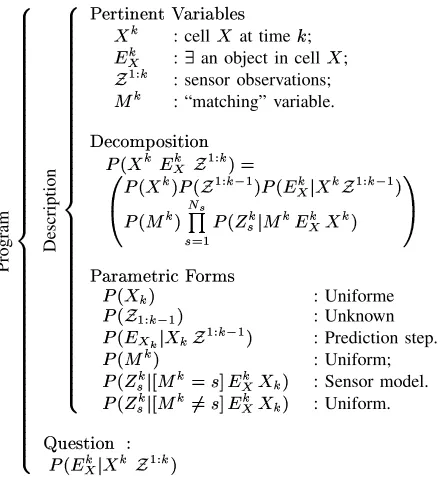
Program "# # # # # # # # # # # # # # # # # # # # # # # # # # # # # # # # # $ # # # # # # # # # # # # # # # # # # # # # # # # # # # # # # # # #% Description "# # # # # # # # # # # # # # # # # # # # # # # # # # # # $ # # # # # # # # # # # # # # # # # # # # # # # # # # # #% &('*),+.-0/'*/1+32 4).-5476980';: <>=
: cell<
at time? ; @ =
A :
B an object in cell
<
;
CED,F=
: sensor observations;
G =
: “matching” variable.
HI';J*KLNMOK:,-P+.-0K/ QERS< = @ =
A
C
D,F =7TU
VW
QERS<>= TQERXC D,F=Y D TQERX@Z= A\[
<=C D,F=Y D T
QER]G^= T_a` b c,d D QER]ef= c [ Gg=h@\= A
<>= T ij
&h4)k4LN'*+,).-0JlK7).LN: QERS< = T : Uniforme QERXC D,F=Y D
T : Unknown QERX@ Am [ < =
CED,F=nY D T
: Prediction step.
QER]G = T : Uniform; QER]e = c [0o G = Ugp*q @ = A < = T
: Sensor model.
QER]e
=
c
[0o
G =srUgp*q @
= A < = T : Uniform. tvu '*:w+.-5K7/yx QERX@ = A [
< = CND,F=
T
Fig. 1: Estimation Step at time z
Fig 1 presents the Bayesian Program for the estimation of the occupancy probability of a cell. To simplify nota-tions, a particular cell of the grid is denoted by a single variable{ , despite the grid is 4-D. The number of sensor
observations at timez is named|~} . One sensor data at
time z is denoted by the variable }
hZ3 7
|
}
. The set of all sensor observation at time z is noted } . The
set of all sensor observations until time z is referred by
the notationZ*
}
.
A variable called the “matching” variable and noted
} is added. Its goal its to specify which observation
of the sensor is currently used to estimate the state of the cell. The result of the inference for the estimation is given by: ] } { } } m m VW ] } {~} } m b } } I } { } ij where
is a normalization constant.
During the inference, the sum on this variable allows to take into account all sensor observations to update the state of one cell.
One has to remark here that the estimation step is performed without explicit association between tracks and observations. Program "# # # # # # # # # # # # # # # # # # # # # # # # # # # # # # # # # # # # # # $ # # # # # # # # # # # # # # # # # # # # # # # # # # # # # # # # # # # # # #% Description "# # # # # # # # # # # # # # # # # # # # # # # # # # # # # # # # # $ # # # # # # # # # # # # # # # # # # # # # # # # # # # # # # # # #% &('*),+.-0/'*/1+32 4).-5476980';: < =
: cell at time? ; @ =
A :
B an object in cell
<
;
< =Y D
: cell at time?\~ ; @Z=Y D
A :
B an object in cell
<
;
CED,F=Y D
: sensor observations until ?(E ; =Y D
: control of the cycab at time ?(E
HI';J*KLNMOK:,-P+.-0K/ QERS< = @ = A < =Y D @ =Y D A C
D,F=Y D
=Y DTU
V
W
QERXC D,F=Y D
TQER =Y DTQERS< =Y D T QERX@Z=Y D
A
[
< =Y DOCED,F=Y D
T
QERS<=
[
<>=Y D I=Y D T QERX@ =
A¡[ @ =Y D
A
< = < =nY D
T
i¢
j
&h4)k4LN'*+,).-0JZlK7).LN: QERXC D,F=Y D
T
: Unknown;
QERI=nY DT
: Uniform;
QERS< =Y D
T : Uniform; QERX@Z=Y D A [ < =Y DOCED,F =nY D T
: estimation at time?(E ; QERS< =
[
< =Y D
T
: dynamic model;
QERX@ = A [
@Z=Y
D
A
< = < =Y D
T
: Dirac.
tvu '*:w+.-5K7/£x QERX@Z=
A [
<>=\C D,F=Y D I=Y D
T
Fig. 2: Prediction Step at time z
To improve the estimation of the grid, we add a prediction step. The goal of the prediction is to provide an a priori knowledge for the estimation. It is based on a dynamical model of the object, which include the vehicle movements, denoted by the variable ¤ }
. Such prediction step is classical in target tracking, in sequential estimation techniques such as the Kalman filter [12]. The corresponding Bayesian program is presented by fig 2.
The result of the inference for the prediction is given by: } { } } ¤ } ¥ ¦ § m¨© ª § m;¨© VW {~} . } {~} * } {~} {~} ¤N} } k } {~} {~} ij (1) where
is a normalization constant.
In general, this expression cannot be determined analyt-ically, and cannot even be computed in real time. Thus an approximate solution of the integral has to be computed. Our approximation algorithm is based on the basic idea that only few points can be used to approximate the integral. Thus, for each cell of the grid at time zE«
, we
compute the probability distribution {¬} {~} ¤N} .
A cell } is drawn according to this probability
distri-bution. Then the cell {¬}
is used to update only the predicted state of the cell h} . The complexity of this
algorithm increases linearly with the number of cells in our grid, and ensures that the most informative points are used to compute the integral appearing in (1).
Thus the estimation of the occupancy grid at timez is
done in two steps. The prediction step uses the estimation step at time z®«
and a dynamical model to compute an
a priori estimate of the grid. Then the estimation step uses this prediction and the sensor observations at timez
to compute the grid.
B. Experimental results
To test the estimation of occupancy grids presented in the previous section, both a simulator and the real Cycab vehicle were used.
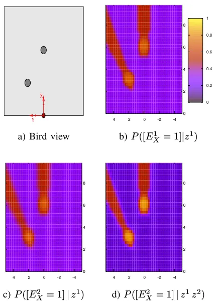
X Y 0 0.2 0.4 0.6 0.8 1 0 2 4 6 8 10 -4 -2 0 2 4
a) Bird view b)k
¯ ° 0 2 4 6 8 10 -4 -2 0 2
4 0
2 4 6 8 10 -4 -2 0 2 4
c)k²± ³ n
.°
d)k²± ´
.°
°±
Fig. 3: First example of grid estimation, for a static scene.
Fig 3 shows first results of estimation and prediction steps, for a static scene. The upper left scheme depicts the situation : two static objects are present in front of the cycab. These two objects are fixed. The cycab is static too. Thus only 2-dimensional grids are depicted, corresponding to object’s position at a null speed. Fig 3b represents the occupancy grid, knowing only the first sen-sor observations. The color corresponds to the probability that a cell is occupied. In this case, the two objects are
detected by the sensor. Consequently, two areas with high occupancy probabilities are visible (orange areas). These probability values depends on probability of detection, probability of false alarm, and on sensor precision. All these characteristics of the sensor are taken into account in the sensor model. The cells hidden by a sensor observation have not been observed. Thus we can not conclude about their occupancy. That explains the two areas of probability values near toµ
P¶ (red areas). Finally, for cells located far
from any sensor observation, the occupancy probability is low (purple areas).
Fig 3c represents the occupancy grid, after the predic-tion step. Because all the scene is static, the result of the prediction step is quite similar to the result of the first estimation step.
Fig 3d represents the occupancy grid after the second sensor observations. Of course, this figure is quite similar to the fig 3b, but two remarks have to be noted:
·
for cells corresponding to an objects, the occupancy probability is higher than in the first estimation. This is due to thea prioriknowledge, which was uniform for the first estimation, and given by the prediction step for the second estimation;
· for cells corresponding to free areas, the occupancy
probability is lower than in the first estimation. This is also due to the prediction step.
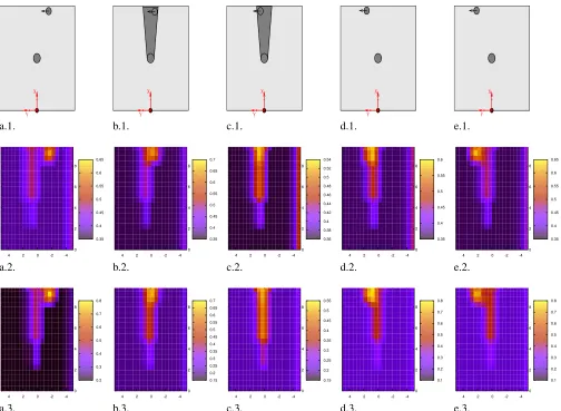
Fig 4 shows an extract of a short sequence of successive prediction and estimation results. Its goal is to demon-strate the robustness of our approach to objects occlusions, without any special logic. The first row describes the situation : the cycab is immobile, a static object is located 5 meters in front of it. A second object is moving from right to left. In the situation depicted by the figs 4b.1 and 4c.1, the moving object is hidden by the static one, and thus is not detected by the Sick laser range finder.
Second and third rows present respectively results of the prediction step and of the estimation step. We choose to represent only the cells of the grids corresponding to relative speed equals to ¸
µ
µ
¸
¹
º 9 µ»!¼
, which is close to the speed of the moving object. The color represents the occupancy probability of the cells. Be careful that the color code is different for each sub-figure.
An area of high occupancy probability is well defined in figs 4a.2 and 4a.3. This area corresponds to the moving object. We remark an area of occupancy probability values equals to µ
¶ , which corresponds to the cells hidden by
the static object. The fig 4b.2 presents the result of the prediction step, based on the grid presented in fig 4a.3, and on a dynamic model. This prediction shows that an object should be located in the area hidden by the static object. Consequently, even if this object is not detected by the laser, an area of high occupancy probability is found in the fig 4b.3. In the same way, the fig 4c.2
predicts that a moving object should be located behind the static object. Thus we still found in fig 4c.3 an area of occupancy probability values greater than 0.5. Of course, the certainty in object presence,i.e.the values of the occupancy probability in the grid, decreases when the object is not observed by the sensor.
In figs 4d.3 and 4e.3, the moving object is no longer hidden by the static object. Thus it is detected by the laser, and the occupancy probability values increase.
Occupancy grids such ones presented in figs 3 and 4 don’t provide precise informations about the vehicle environment. In particular, the number of objects is not estimated. Thus one can think that they are useless in the automotive context.
The next section shows that occupancy grids provide enough information about the environment to perform basic and vital behaviors. The goal is to control the cycab in order to avoid “hazardous” obstacles of the environment.
V. LONGITUDINALCONTROL OF THECYCAB
As mentioned in [2], the cell state can be used to encode a number of properties of the robot environment. Properties of interest for robot programming could include occupancy, observability, reachability, etc. In the previous section, it was used to encode the occupancy of the cell. In this section, we show how it could be used to encode the dangerof the cell. By this way, the cycab is longitudinally controlled by combining the occupancy and the danger of all cells.
A. Estimation of danger
For each cell of the grid, the probability that this cell is hazardous is estimated. This estimation is done without considering the occupancy probability of the cell. Thus we estimate the probability distribution ]½
}
{}
for
each cell { of the cycab environment.
½
}
is a boolean
variable that indicates whether the cell{ is hazardous or
not.
As a cell { of our grid represents a position and
a velocity, the TCPA (Time to the Closest Point of Approach) and the DCPA (Distance to the Closest Point of Approach) can be estimated for each cell. Thanks to TCPA and DCPA, the estimation of the danger is more intuitive than if we had considered directly the relative speed encoded in the grid : the lower the DCPA and the shorter the TCPA, the more hazardous the cell.
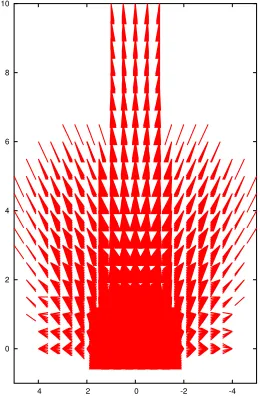
Fig 5 shows the cells for which danger probability is greater thanµ
0¾ . Each cell is modeled with an arrow: the
beginning of the arrow indicates the position, the length and the direction indicates the speed. First, we can see that any cell located close to the cycab is considered as hazardous, whatever the speed is. For other locations, the more hazardous cells are those which speed is in the
X Y X Y X Y X Y X Y
a.1. b.1. c.1. d.1. e.1.
0.35 0.4 0.45 0.5 0.55 0.6 0.65 0 2 4 6 8 10 -4 -2 0 2 4 0.35 0.4 0.45 0.5 0.55 0.6 0.65 0.7 0 2 4 6 8 10 -4 -2 0 2 4 0.36 0.38 0.4 0.42 0.44 0.46 0.48 0.5 0.52 0.54 0 2 4 6 8 10 -4 -2 0 2 4 0.35 0.4 0.45 0.5 0.55 0.6 0 2 4 6 8 10 -4 -2 0 2 4 0.35 0.4 0.45 0.5 0.55 0.6 0.65 0 2 4 6 8 10 -4 -2 0 2 4
a.2. b.2. c.2. d.2. e.2.
0.2 0.3 0.4 0.5 0.6 0.7 0.8 0 2 4 6 8 10 -4 -2 0 2 4 0.15 0.2 0.25 0.3 0.35 0.4 0.45 0.5 0.55 0.6 0.65 0.7 0 2 4 6 8 10 -4 -2 0 2 4 0.15 0.2 0.25 0.3 0.35 0.4 0.45 0.5 0.55 0 2 4 6 8 10 -4 -2 0 2 4 0.1 0.2 0.3 0.4 0.5 0.6 0.7 0.8 0 2 4 6 8 10 -4 -2 0 2 4 0.1 0.2 0.3 0.4 0.5 0.6 0.7 0.8 0 2 4 6 8 10 -4 -2 0 2 4
a.3. b.3. c.3. d.3. e.3.
Fig. 4: A short sequence of a dynamic scene. The first row describes the situation : a moving object is temporary hidden by a static object. The second row shows the predicted occupancy grids, and the third row the result of the estimation step. The grids are 2-dimensional, and shows the probabilityk
} ³ n ¹ ¸ µ ¸ ¹ ³ ¿ µ .
direction of the cycab. As we consider relative speed in the danger grid, this grid does not depend of the actual cycab velocity.
B. Control of the cycab
Our goal here is to control the longitudinal speed of the cycab, in order to avoid moving objects. The behavior we want the cycab to adopt is very simplistic : brake or accelerate whether it feels itself in danger or not.
To program this behavior, we consider simultaneously for each cell{ of the environment its danger probability
(given by the distribution ]½
}
{~} explained in the
V-A) and its occupancy probability (given by the distri-bution] } * } {~}
explained in the IV). We look for the most hazardous cell that is considered as occupied, that is:ÀÁÂ
mÄÃ ]½ } { } wÅ ~] } { } IÆ µ ¶OÇ9
Then the longitudinal acceleration of the cycab is decided according to this level of danger and to its actual velocity. The four possible commands are : emergency brake, brake, accelerate or keep the same velocity.
Fig 6 illustrates this basic control of the cycab. In this example, a pedestrian appears suddendly. The cycab brakes to avoid him. This basic control allows the cycab to adopt secure behaviors, such as keeping a safety distance from a car preceding itself. Stop and go is also en-sured with this control. Videos illustrating these behaviors should be available athttp://www.inrialpes.fr/ sharp/people/coue/.
What it is to be noted here is that no decision is taken before the choice of the command applied to the cycab. In particular, we do not know the exact number of object located in the cycab environment. Furthermore, exact positions and velocity of these objects are not estimated.
Fig. 6: Example of the cycab control.
0 2 4 6 8 10
-4 -2 0 2 4
Fig. 5: Cells of high danger probabilities. For each posi-tion, arrows model the speed.
VI. CONCLUSION
This paper addressed the problem of 4-D occupancy grid estimation in an automotive context. According to us, this grid can be an alternative to complex multi-target tracking algorithms for applications which does not require information such as the number of objects. To improve the estimation, a prediction step has been added. Thanks to this prediction, the estimation of the grid is robust to temporary occlusions between moving objects. To validate the approach, an application involving the Cy-cab vehicle has been shown. The CyCy-cab is longitudinally controlled in order to avoid obstacles. This basic behavior is obtained by combining the occupancy probability and the danger probability of each cell of the grid.
Future developments will include: a) improvements of the approximation algorithm for the prediction step. These improvements should allow to estimate a bigger grid, which is required to control a car in urban areas. b) fu-sion of the occupancy grid with higher-level information, such as GPS maps, to better estimate the danger of the situation.
Acknowledgements. This work was partially
sup-ported by the European project IST-1999-12224 “Sens-ing of Car Environment at Low Speed Driv“Sens-ing” (http://www.carsense.org).
VII. REFERENCES
[1] H.P. Moravec. Sensor fusion in certainty grids for mobile robots. AI Magazine, 9(2), 1988.
[2] A. Elfes. Using occupancy grids for mobile robot perception and navigation. IEEE Computer, Spe-cial Issue on Autonomous Intelligent Machines, Juin 1989.
[3] O. Lebeltel, P. Bessi`ere, J. Diard, and E. Mazer. Bayesian robots programming. Research Report 1, Les Cahiers du Laboratoire Leibniz, Grenoble (FR), May 2000.
[4] 0 Lebeltel, P. Bessi`ere, J. Diard, and E. Mazer. Bayesian robot programming. Autonomous Robots, 2003. to appear.
[5] E. T. Jaynes. Probability theory: the logic of sci-ence. in press, on-line news at http://bayes. wustl.edu, 1995.
[6] G. Cooper. The computational complexity of prob-abilistic inference using bayesian belief network. Artificial Intelligence, 42(2-3), 1990.
[7] Y. Bar-Shalom and X. Li. Multitarget-Multisensor Tracking: Principles and Techniques. Artech House, 1995.
[8] H. Gauvrit, J.P. Le Cadre, and C Jauffret. A formu-lation of multitarget tracking as an incomplete data problem. IEEE Trans. on Aerospace and Electronic Systems, 33(4), October 1997.
[9] R.L. Streit and T.E. Luginbuhl. Probabilistic multi-hypothesis tracking. Technical Report 10,428, Naval Undersea Warfare Center Division Newport, 1995. [10] S. Blackman and R. Popoli. Design and Analysis of
Modern Tracking Systems. Artech House, 2000. [11] S. Thrun. Robotic mapping: A survey. InExploring
Artificial Intelligence in the New Millenium. Morgan Kaufmann, 2002.
[12] R.E. Kalman. A new approach to linear filtering and predictions problems. Journal of Basic Engineering, March 1960.