Volume 2008, Article ID 596989,16pages doi:10.1155/2008/596989
Research Article
3D Shape-Encoded Particle Filter for Object Tracking and
Its Application to Human Body Tracking
H. Moon1and R. Chellappa2
1VideoMining Corporation, 403 South Allen Street, Suite 101, State College, PA 16801, USA
2Department of Electrical and Computer Engineering, University of Maryland, College Park, MD 20742, USA
Correspondence should be addressed to H. Moon,[email protected]
Received 1 February 2007; Revised 14 July 2007; Accepted 25 November 2007
Recommended by Maja Pantic
We present a nonlinear state estimation approach using particle filters, for tracking objects whose approximate 3D shapes are known. The unnormalized conditional density for the solution to the nonlinear filtering problem leads to the Zakai equation, and is realized by the weights of the particles. The weight of a particle represents its geometric and temporal fit, which is computed bottom-up from the raw image using a shape-encoded filter. The main contribution of the paper is the design of smoothing filters for feature extraction combined with the adoption of unnormalized conditional density weights. The “shape filter” has the overall form of the predicted 2D projection of the 3D model, while the cross-section of the filter is designed to collect the gradient responses along the shape. The 3D-model-based representation is designed to emphasize the changes in 2D object shape due to motion, while de-emphasizing the variations due to lighting and other imaging conditions. We have found that the set of sparse measurements using a relatively small number of particles is able to approximate the high-dimensional state distribution very effectively. As a measure to stabilize the tracking, the amount of random diffusion is effectively adjusted using a Kalman updating of the covariance matrix. For a complex problem of human body tracking, we have successfully employed constraints derived from joint angles and walking motion.
Copyright © 2008 H. Moon and R. Chellappa. This is an open access article distributed under the Creative Commons Attribution License, which permits unrestricted use, distribution, and reproduction in any medium, provided the original work is properly cited.
1. INTRODUCTION
Using object shape information for tracking is useful when it is difficult to extract reliable features for tracking and mo-tion computamo-tion. In many cases, an object in a video se-quence constitutes aperceptual unit which can be approxi-mated by a limited set of shapes. Many man-made objects provide such examples. A human body can also be decom-posed into simple shapes. For tracking or recognition of hu-man activities, appearance features are often too variable, and local features are noisy and not reliable for establish-ing temporal correspondences. Shape constraints also pro-vide strong clues about object pose while the object is mov-ing. “Shape” in this context refers to persistent geometric im-age signature, such as ellipsoidal human head boundary, par-allel lines for the boundary of limbs, or facial features.
We model a human body using simple quadratic solids; the 2D projection of the solids constitutes the “shapes” to be tracked. The image gradient signature of a shape is modeled using the optimal shape operator that was introduced in [1].
The adoption of quadratic solids for modeling parts facili-tates the computation of the shape operator. The responses of an image frame to a set of shape operators having certain ranges of pose and size parameters are used as observations in a nonlinear state space formulation, to guide object track-ing and motion estimation. The magnitudes of the responses are accurate and robust to noise, and they enable reliable esti-mation of geometric parameters (location, orientation, size) and provide a strong temporal correspondence for tracking the object in subsequent frames.
sampling for accurate object localization and effective search for the state parameters. Reference [9] used the framework of sequential importance sampling [5] to solve the problem of simultaneous object tracking and verification. Reference [10] also employed particle filtering for the 3D tracking of a walking person.
In our approach, the functional relation between the ge-ometric parameter space and the image space makes the ob-servation process highly nonlinear. There is a generalization of the Kalman filter to the nonlinear framework, by Zakai [11]. They derived an equation that incorporates both dy-namic and observation equations, and which, if solved, en-ables the temporal propagation of the probability of the states conditioned on the observations. Reference [12] introduced the Zakai equation to image analysis problems.
As derived in filtering theory, the unnormalized condi-tional density is a solution to the Zakai equation. The so-lution is in general not available in a closed form; we em-ploy a branching particle method to solve the filtering prob-lem. The system of particles that simulates the conditional density of states is found [13] to converge to the target dis-tribution. The proposed measurement process—shape filter response—contributes to the accurate computation of the weights. We also have a unique way of computing the unnor-malized conditional density used for computing the weights, that takes into account both geometric fit of the data and temporal coherenceof the motion. The method of estimat-ing the number of offsprings using randomized sampling is also designed to be optimal, while the total number of sam-ples is fixed in resampling approaches. It has been shown in [14] that the particle method is superior to the resampling method in terms of large sample behavior.
After branching, the particles follow the system dynam-ics plus random perturbation. As we cannot assume any par-ticular motion model in most applications, we employ an approximate second-order motion prediction. The predic-tion is modified by a random search to minimize the pre-diction error. The amount of random diffusion has to be determined, which we found to be crucial for stable track-ing. The state error covariance matrix is computed by sub-tracting the prior covariance matrix from the posterior co-variance matrix, according to the Kalman filter time update equations. We found that the computed covariances adapt to the motion, and they are usually very small; nevertheless, this method of computing the diffusion shows noticeable im-provements in tracking and pose estimation.
We first applied this method of shape tracking to the problem of human head tracking, and later to the full body tracking in a monocular video sequence. For head tracking, the head is modeled as a 3D ellipsoid, and the motion of the head as rotation combined with translation, having a total of six degrees of freedom. Facial features are approximated as simple geometric curves; we compute the operators for tracking the features given the hypothetical pose of the head and the positions and sizes of the features, by using the in-verse camera projection. Experiments show that the particles are able to track and estimate the head motion accurately. In addition, the three parameters representing the size of the ellipsoid are free, along with the distance from the ellipsoid
to the camera. The proposed algorithm simultaneously esti-mates the size, pose, and location (up to scale) of the ellip-soid.
We also extended our application to full body tracking of a walking person when the person is walking approximately perpendicular to the camera axis. The body is modeled as be-ing composed of simple geometric surfaces: ellipsoid for the head and truncated cones for the limbs. We also have added texture information of the parts in addition to the shape. We have found that the addition of texture cue helps the track-ing in a meantrack-ingful way. The kinematic model of the body constrains the pose of the body within physically possible range, which also limits the search space for tracking. The full body tracking is a very hard problem due to complex mo-tion, high dimensionality, and self-occlusion. While the pro-posed method cannot completely solve the problem, we have found that the constraint provided by the shape and texture cues, the employment of a smoothing filter to extract reliable features, and the adoption of weight function derived from filtering theory make the tracking of walking person more manageable.
We first introduce a representation based on quadratic surfaces to compute the shape operator (Section 2). In Section 3, the tracking of a human is formulated as a non-linear filtering problem. The subsections cover the details of branching particle method. Section 4presents the applica-tion of human head tracking. The tracking of human walking motion is detailed inSection 5.
2. SHAPE AND MEASUREMENTS
In the general context of object recognition or tracking, the outline of an object gives a compact representation of the ob-ject, whereas color or texture information is usually highly variable with different instances of objects or imaging en-vironments. The boundary contour of an object gives clues for detection/recognition that are almost invariant to imag-ing conditions except for the pose.
On the other hand, methods for appearance-based track-ing ustrack-ing a linear subspace representation [15] or an ob-ject template [16] have been considered. While these meth-ods use holistic representations of object intensity structure, which can be effectively used to recognize or classify objects in video, they have limited ability to represent and compute changes in object pose. Nevertheless, the use of a global ob-ject representation has the advantage that it helps to maintain the temporal correspondence of features. The addition of learned representation of object images will provide a pow-erful edge to object tracking, as shown in [17]. The proposed work, however, ventures to improve object tracking from the model-based front.
tracking using 3D deformable model and optical flow com-putation using 3D shape constraints, and presents an appli-cation to face tracking. Reference [20] shows how the dynam-ical shape priors, represented using level sets, provide strong constraints for segmenting/tracking deformable shapes un-der severe noise and occlusions. Shape constraints provide tighter constraints on object configuration than point fea-tures do; the deformation of a shape due to changes in object pose or camera parameters (e.g., focal length) provides bet-ter clues about these paramebet-ters, while local point features (e.g., end-points, vertices, junctions), often cannot. We have observed that shape constraints, being global, effectively sta-bilize tracking when the tracking deviates from the correct course after a rapid motion.
We make use of 3D shape model, combined with the boundary gradient information extracted using this model, to track body motion. Given the predicted size, position, and pose of the body parts, the projection of the model is com-pared to the image using the set of shape filters. Using the op-timal shape detection and localization technique derived in [1], the responses of the shape operators provide the tracker with an accurate geometrical fit of the model to the data, and a strong temporal correspondence between frames.
We now briefly introduce the image operator we use for measuring the model fit. We then introduce how the use of 3D solids facilitates the construction of shape filter for two kinds of shape cues: the body silhouette and facial features. The body tracking makes use of boundary shape, while head tracking is accomplished using the positions and shapes of facial features.
2.1. Shape filters to measure shape match
In [1], the optimal one-dimensional smoothing operator, designed to minimize the sum of noise response power and step edge response error, was shown to be gσ(s) = (1/σ) exp(−|s|/σ). Then the shape operator for an arbitrary shape regionD, whose boundary is the shape contourC, is defined by
G(x)=gσ
l(x), (1)
where the level functionlcan be implemented by
l(x)=
⎧ ⎪ ⎨ ⎪ ⎩
+min
z∈Cx−z forx∈D,
−min
z∈Cx−z forx∈D
c. (2)
The level function lsimply takes the role of supplying the distance function to the shape contourC.lcan have a reg-ular parametric form (e.g., quadratic), when the shape con-tourC is a parametric curve.Figure 4shows a shape oper-ator for a circular arc feature, matched to an eye outline or eyebrow in the head tracking problem. The operator is de-signed to achieve good shape detection and localization per-formance. The detection performance is equivalent to the ac-curacy of the filter response, while the localization perfor-mance is closely related to the recognition/discrimination of the shape.
2.2. 3D body and head model
The 3D model of the body consists of truncated cones (trunk and limbs) and an ellipsoid (head). The body contour shape is represented by the distance function around the contour; the equation is derived by combining the quadratic equation for the solids and the perspective projection equation.
Let the 3D geometry of a body part be approximated by a quadratic surface parameterized by (pose,size)=ξ:
Mξ(p)=Mξ(x,y,z)=0, (3) where p = (x,y,z) is any point on the solid. Note that throughout the paper M = Mξ will denote both the quadratic equation that defines the surface and the surface itself. The image plane coordinatesP = (X,Y) of the pro-jection ofpare computed usingX/ f =x/zandY/ f = y/z, where f is the focal length. We construct the shape opera-tor of the projection ofMξ. Given a pointP=(X,Y) in the image plane, let the corresponding point onMξbe (x,y,z). Then we have a quadratic equation with respect to depthz:
Mξ
X fz,
Y fz,z
Δ
=aX,Y,fz2+bX,Y,fz+cX,Y,f =0, (4)
wherea = aX,Y,f,b = bX,Y,f,c= cX,Y,f are constants that depend onX,Y,f. The distance from (X,Y) to the bound-ary contour of the projection ofMξ is approximated by the determinant
d(P)=df(x,y)=−b+
√
b2−4ac
2a , (5)
assuming that (X,Y) is close to the boundary contour. The shape operator for a given shape regionDis then defined by
G(P)=gσ
d(P), (6) wheregσis as defined inSection 2.1.
2.3. Facial feature model
Head tracking is guided by the intensity signatures of distinc-tive features of the face, such as eyes, eyebrows, and mouth. The head surface is approximated by an ellipsoid (Figure 1); the eyes and eyebrows are modeled by combinations of cir-cular arcs, which are assumed to be drawn on the ellipsoid (Figure 2). Using these simple models of the head and facial features, we are able to compute the expected feature signa-tures and corresponding shape operators.
2.3.1. Ellipsoidal head model
We provide a detailed description of the 3D representation of facial features, which will also serve as an example of the formulation laid out in the previous section. We model the head as an ellipsoid inxyz space, withz being the camera axis:
Mξ(x,y,z)=MRx,Ry,Rz,Cx,Cy,Cz(x,y,z)
Δ
=
x−Cx
2
R2 x
+
y−Cy
2
R2 y
+
z−Cz
2
R2 z
n
θy
Ry
Rx
(Cx,Cy,Cz)
Rz
a=(Ax,Ay,Az) θ x
θz
Figure1: Rotational motion model of the head.
El Ir
(Bh, Bv)
(Ih, Iv) Ev Eh Origin
Ew
(Mh, Mv)
Figure2: Ellipsoidal head model and the parameterization of facial features.
We represent the pose of the head by three rotation an-gles (θx,θy,θz):θxandθz measure the rotation of the head axis n, and the rotation of the head around n is denoted by θy(= θn). The center of rotation is assumed to be near the bottom of the ellipsoid (corresponding to the rotation around the neck), denoted bya=(ax,ay,az), which is mea-sured from (Cx,Cy,Cz) for convenience. Since the rotation ofn and the rotation of the head around it are commuta-tive, we can think of any change of head pose as rotation around the yaxis, followed by “tilting” of the axis. LetQx,
Qy, and Qz be rotation matrices around x, y, and z axes, respectively. Let p = (x,y,z) be any point on the ellipsoid
MRx,Ry,Rz,Cx,Cy,Cz(x,y,z). p moves to p = (x,y,z) under
rotationQyfollowed by rotationsQxandQz:
p=QzQxQy(p−b−a) +a+b. (8)
Note thatb = b(Cx,Cy,Cz) = (Cx,Cy,Cz) represents the
posi-tion of the ellipsoid before the rotaposi-tion.
The eyes are undoubtedly the most prominent features of a human face. The round curves made by the upper eyelid and the circular iris give unique signatures which are pre-served under changes in illumination and facial expression. Features such as the eyebrows and mouth can also be utilized. Circles or circular arcs on the ellipsoid approximate these fea-ture curves. We parameterize the positions of these feafea-tures by using the spherical coordinate system (azimuth,altitude) on the ellipsoid. A circle on the ellipsoid is given by the inter-section of a sphere centered at a point on the ellipsoid with the ellipsoid itself. We typically used 22 parameters, which include 6 pose/position parameters.
2.3.2. Camera model and filter construction
We combine the head model and the camera model to pute the depth of each point on the face, so that we can com-pute the inverse projection and construct the corresponding operator.Figure 3illustrates the scheme. The center of per-spective projection is (0, 0, 0) and the image plane isz = f. LetP = (X,Y) be the projection of p = (x,y,z) on the ellipsoid. These two points are related by
X f =
x z,
Y f =
y
z. (9)
Given ξ = (Cx,Cy,Cz,θx,θy,θz,ν), the geometric parame-ters of the head and features (simply denoted byν), we need to compute the inverse projection on the ellipsoid to con-struct the shape operator. Suppose the feature curve on the ellipsoid is the intersection (with the ellipsoid) of the circle (x,y,z)−(eξx,eξy,eξz)2 =Rξ
2
e centered at (eξx,eξy,eξz) (which is also on the surface). LetP=(X,Y) be any point in the im-age. The inverse projection ofPis the line defined by (9). The point (x,y,z) on the ellipsoid is computed by solving (9) along with the quadratic equationMRx,Ry,Rz,Cx,Cy,Cz(x,y,z)=
0. This solution exists and is unique, since we seek the solu-tion on the visible side of the ellipsoid. The point (x,y,z) on the reference ellipsoidM0,0,0,Cx,Cy,Cz(x,y,z)=0 is computed
using the inverse operation of (7).
If we define the mapping from (X,Y) to (x,y,z) by
ρ(X,Y)=Δ (x,y,z)=Δ ρx(X,Y),ρy(X,Y),ρz(X,Y)
, we can construct the shape filter as
Gξ(X,Y)=gσ
ρ(X,Y)−exξ,eξy,eξz 2
−Rξe2
. (10)
(0, 0,Cz)
(Cx,Cy,Cz)
(Cx,Cy,Cz)
P=(x,y,z) P=(x,y,z) (0, 0,f)
(X,Y) (0, 0, 0)
Figure3: Perspective projection model of the camera.
2.4. The measurement equation
The response of the local imageI to the shape operatorGα that represents an object having geometric configurationαis
rα=
Gα(u)I(u)du. (11)
If we assume that the image is corrupted by noisen(t), then the observationyαis given by
yα=
Gα(u)I(u)du+
Gα(u)n(u)du=rα+n, (12)
where nis the noise response. Since we sample the obser-vations yα over the course of time, we formally denote the observation process by
Yt=
t
0h(αs)ds+Vt, (13) where we have definedh(αs)=Δrαs.
We assume that the observation noise is a standard Brow-nian motionVt. The observation noise, though correlated in the spatial dimension, is independent in the temporal di-mension. Since the noise structure ofnis homogeneous with respect to geometric parameters, we can assume that the ob-servation noise is a standard Brownian motionVt.
While the proposed method belongs to the family of feature-based motion computation methods, in that it relies on boundary gradient information, we do not use detected features. The gradient information is computed bottom-up from the raw intensity map using the shape filters. The boundary gradient information is retained for computing the fit to the model shape. If we try to extract gradient fea-tures using an edge detector, some of the boundary edge in-formation may be lost due to thresholding. The total edge
30 25 20
15 10 5
0 60
50 40 30 20 10 0
−0.1
−0.05
0 0.05 0.1
Figure4: Shape filter: the shape is matched to a circular arc to de-tect the eye outline, and the cross-section is designed to dede-tect the intensity change along the boundary.
The shape filter can be constructed for arbitrary contours, so that more accurate fitting can be carried out.
3. THE ZAKAI EQUATION AND THE BRANCHING PARTICLE METHOD
3.1. The Zakai equation
We start the formulation in a more general context to intro-duce the Zakai equation and the branching particle method. The state vectorXt∈Ωrepresenting the geometric parame-ters of an object is governed by the equation
dXt= f
Xt
dt+σXt
dWt. (14) Here Wt is a Brownian motion, and σ = σ(Xt) models the state noise structure in a standard (probability) measure space (Ω,F,P). Since we will not be using any lineariza-tion in the computalineariza-tion, the transfer funclineariza-tion f can have a very general form. The state vector should be of the form
Xt = (αt,βt), whereαt is the vector representing the geom-etry (position, pose, etc.) of the object andβtis the motion parameter vector.
The tracking problem is solved if we can compute the state updates, given information from the observations in (10). We are interested in estimating some statisticφof the states, of the form
πt(φ)=Δ E
φXtYt
(15)
given the observation history Yt up to t. Zakai [11] has shown that the unnormalized conditional densitypt(φ) sat-isfies a partial differential equation, usually called the Zakai equation:
d pt(φ)=pt(Aφ)dt+pt(h∗φ)dYt. (16) HereAis a differential operator involving the state dynamics
f and the state noise structuresσ(Xt) anddWt. Note that the equation is equivalent to the pair of state equation (14) and observation equation (10).
3.2. The branching particle algorithm
It is known in nonlinear filtering theory [22] that the un-normalized optimal filterpt(φ), which is a solution to (16), is given by
E
φXt
exp t
0h ∗X
s
dYx− 1 2
t
0h ∗X
s
hXs
ds Yt
,
(17)
where the expectation is taken with respect to the measureP
which makesYta Brownian motion (cf. [22]). This equation is merely a formal expression, because one needs to evaluate the integrationE[·|Yt] with respect to the measureP. How-ever, this equation provides a recursive relation to derive a numerical solution; we will construct a sequence of branch-ing particle systems Un as in [13] which can be proved to approach the solutionpt, that is, limn→∞Un(t)=pt.
Let{Un(t),Ft; 0 ≤t ≤ 1}be a sequence of branching particle systems on (Ω,F,P).
Initial condition
(0) Un(t) is the empirical measure ofnparticles of mass 1/n, that is,Un(t)=(1/n)
n
i=1δxn
i, wherex
n
i ∈E, for everyi,n∈N, andδxn
i(x) is a delta function centered
atxn i.
Evolution in the interval[i/n, (i+ 1)/n],i=0, 1,. . .,n−1 (1) At time i/n, the process consists of the occupation
measure ofmn(i/n) particles of mass 1/n (mn(t) de-notes the number of particles alive at timet).
(2) During the interval, the particles move independently with the same law as in the system dynamics equation (14). LetZ(s),s∈[i/n, (i+ 1)/n), be the trajectory of a generic particle during this interval.
(3) Att=(i+ 1)/n, each particle branches intoξi
nparticles with a mechanism depending on its trajectory in the interval. The mean number of offsprings for a particle is
μin=E
ξni
=exp h∗Z(t)dYt− 1 2
h∗hZ(t)dt
(18)
so that the varianceνi
n(V) is minimal, where the vari-ance occurs due to the off-rounding ofνi
n(V) to com-pute the integer value ξi
n. The symbol ∗ represents complex conjugate (transpose for the real-valued case) here and throughout the paper. More specifically, we determine the numberξi
nof offsprings by
ξi n= ⎧ ⎨ ⎩ μi n
with probabilityμi n− μi n , μi n
+ 1 with probability 1−μi n+ μi n , (19)
where [] is the rounding operator.
Note that the integrals in (18) are along the path of the particlesZ(t). In the proposed visual tracking application, we only apply the branching mechanism only once per obser-vation interval (between image frames). We take advantage of the branching particle method in two aspects: the recur-sive unnormalized conditional density filter (its implementa-tion is described inSection 3.4) and the minimum variance branching scheme.
3.3. Time update of the state
Another feature of the proposed method is the use of effective prediction and diffusion strategies. Step 2 of the algorithm is based on an unrealistic assumption that we have a partic-ular state transition function and an error covariance ma-trix. We only assume a second-order motion model, and re-cursively estimate the motion and diffusion parameters. We represent the dynamical equation as a discrete-time process:
to one of recursively estimating the motion parameters us-ing a system identification technique. In fact, [23] achieves better global stability of the EKF by adding an extra term in the Kalman gain computation. This term forces the state to be updated so that the prediction error with respect to these parameters is minimized. The proposed random search is closely analogous to this scheme in that it adjusts the dis-placement to ensure the maximum observation likelihood:
dk=arg maxd
h(xk+d)ds.
The random search is performed by first generating a number of particles around the predicted state, according to a Gaussian distribution. The spread of the Gaussian distri-bution is empirically determined. Then the shape fitness (the response to the corresponding shape operator) of each par-ticle is computed. The parpar-ticle having the maximum fitness is chosen as the adjusted predicted state. This scheme is dif-ferent from the original particle process, in that the particles for random search are used once in the given cycle and dis-carded. The particle fitness is simply the shape filter response, not the filtering weight (the unnormalized conditional den-sity).
The original weight equation is supposed to adjust the weights of the sampled particles (diffused around the dicted state) based on the observation. However, if the pre-diction is offby too much (e.g., when the prediction falls at the tail of the true distribution), it introduces significant bias. The original branching particle framework suggests applying the branching mechanism multiple times within the obser-vation interval, though it would be too costly to implement. The prediction adjustment can also be seen as a cheaper al-ternative to achieve the same goal. This seemingly simple ad-dition of a prediction adjustment is found to significantly in-crease stability.
Borrowing notation from the Kalman filter literature, the time update step yields the prior estimate of the state and the covariance matrix:
xk−+1=xk+dk,
P−k+1=Pk+Σk.
(20)
HerexkandPkdenote the posterior estimates after the mea-surement update (the application of the Kalman gain), which is equivalent to the observation and branching steps in the branching particle algorithm. The a priorianda posteriori error covariance matrices are formally defined as
Pk−=E[(x−k −xk)(x−k −xk)T],
Pk=E[(xk−xk)(xk−xk)T].
(21)
These matrices are estimated by bootstrapping the particles
xk and the prior/posterior state estimates (x−k,xk) into the above expressions. We use the error covariance estimated from the particles at timek−1 for the diffusion at timek
by (20):
Σk=Σk−1=P−k −Pk−1 (22) since we can only compute (21) after the diffusion and the measurement update. The subtraction of the prior
covari-ance matrix ensures that the perturbation due to the diff u-sion is measured. If the particles are perturbed according to
Pk, they are bound to divergence because of the addition of unnecessary uncertainties at each step.Σkis positive semidef-inite sincexk=E[xk].
We have observed that the diffusion matrix adapts to the motion. If the state vector moves fast in a certain direc-tion, the prediction based on the previous estimates moves away from the correct value. The difference between the pre-dicted distribution (P−) and the measured distribution (P) becomes large, so that more diffusion is assigned to that di-rection. This characteristic of the diffusion method translates into an efficient search for the motion parameters. This prop-erty also helps the static (model) parameter values to stabi-lize. Many of the geometric parameters of the object model are initially chosen by crude guesses, and they are adjusted as more information comes in. Since the amount of perturba-tion is tuned according to the goodness of fit, the parameter value eventually settles down. If a stabilized value turns out to be inaccurate as the pose changes, more perturbation due to the mismatch causes the parameter to escape from a lo-cal maximum and wander around looking for a better value. This stabilizing characteristic is observed in experiments, and will be explained in a later section.
An alternative way of handling the state prediction is to include the velocity parameters into the state vector and propagate them with model and pose parameters. We found that estimating the dynamic parameters using the prior esti-mates of the states gives much better performance, in the ap-plications studied here. The increased dimensionality is one of the possible causes, and one can also suspect that this is due to the extra degree of randomness caused by perturbing the velocity parameter.
3.4. Measurement update
The “observation likelihood” term inside the exponential in (18) can be rearranged as
−1 2
t
0
h∗−dYs∗
h−dYs
+1 2
t
0dY ∗
s dYs. (23) The first term measures the disparity between the predicted and measured responses, which forces temporal invariance of the shape signature between the current and previous frames. The second term is the response strength, representing how close the data is to the model shape in the current frame. We can compute the weights accurately without any loss of edge information, as explained inSection 2.
forhandRforY, we compute the unnormalized conditional density (18) by
exp
HxkRxk−
1 2H
2
xk =exp
Rxk−1Rxk−
1 2R
2
xk−1 (24)
by replacingHxkwithRxk−1. We have found that this unique way of computing the unnormalized conditional density is essential for propagating the posterior density. We experi-mented with other ad hoc expressions for computing the weights by trying many combinations of terms in the above equation; they were all unsuccessful.
Figure 5illustrates how the particles are processed at each stage of the branching particle algorithm. The sizes of the dots represent the weights, and the dominant particles are marked with white dots, which yield more offsprings after branching than the other “weaker” particles. The values of the state vectors are preserved until the last stage where the state vectors go through a uniform displacement and a ran-dom perturbation.
4. HEAD TRACKING
We have first applied the proposed method to the problem of 3D head tracking. There have been successful appearance-based tracking algorithms [24,25], using texture mapping on cylindrical head model. We use feature shape information— global arrangement and local shapes of facial features to guide tracking. The set of shape filters constructed from the 3D head and facial feature model (Section 2) is used to ex-tract image features. The problem is relatively manageable because the head pose change is almost rigid; one only needs to take into account the local deformation due to facial ex-pression.
The initial distribution is realized by uniformly sampling parameter vectors from a suitably chosen 22-dimensional cu-bic region in parameter space, and by thresholding them by shape filter responses. We used about 200 particles in most experiments, and observed that further increasing the num-ber of particles did not make a noticeable difference in per-formance.
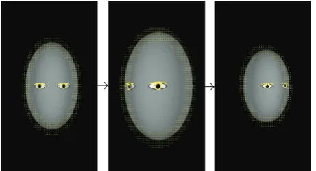
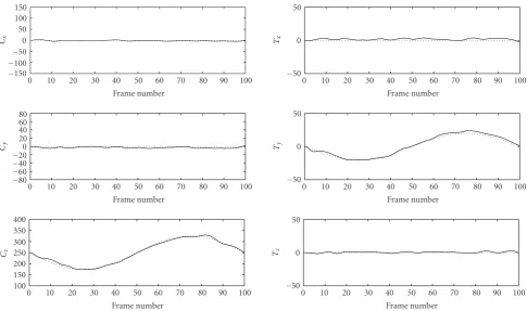
Experiments on synthetic data show good tracking of fa-cial features and accurate head pose estimates, as shown in Figure 6. The head is “shaking” while moving back and forth. The plots inFigure 7compare the estimated translation and rotation parameters with real values.
We have tested many human head motion sequences, and the algorithm achieved reliable tracking.Figure 8shows an example, where the person repeatedly moves his head left and right, and the rotation of the head is naturally coupled with translation. The principal motions are x-translation andy-rotation; smally-translation andz-rotation are added since the head motion is caused by the “swing” of the up-per body while sitting on a chair. Tracking and motion esti-mation would be easier if we only allowed rotation in which the axis of rotation is fixed around the bottom of the up-per body. However, allowing all degrees of freedom yielded good performance. The plots of the estimated parameters are given in the left column ofFigure 9(b). The global motion (Cx,Ty,Cy,Tz) shows coherent periodicity.
Measurement Branching Drift + diffusion
xk− xk xk−+1=xk+dk
Figure5: Schematic diagram of branching particle method.
Figure 6: Sampled frames from a synthetic sequence. The head is moving back and forth (translation) while “shaking” (rotation). The estimated head pose and location and the facial features are marked.
0 10 20 30 40 50 60 70 80 90 100 Frame number
−150
−100
−50
0 50 100 150
Cx
0 10 20 30 40 50 60 70 80 90 100
Frame number
−50
0 50
Tx
0 10 20 30 40 50 60 70 80 90 100
Frame number
−80
−60
−40
−20
0 20 40 60 80
Cy
0 10 20 30 40 50 60 70 80 90 100
Frame number
−50
0 50
Ty
0 10 20 30 40 50 60 70 80 90 100
Frame number 100
150 200 250 300 350 400
Cz
0 10 20 30 40 50 60 70 80 90 100
Frame number
−50
0 50
Tz
Figure7: Estimated parameters for synthetic data (left column: translational motion; right column: rotational motion). The dotted lines are the real parameters used to generate the motion.
more “cautious” in exploring the parameter space, while the fixed diffusion method “ventures” into parameter space us-ing larger steps. The amount of diffusion in the case of the adaptive method is much smaller than in the case of a (work-ing) fixed method.
The estimates of model parameters are also shown in this figure. In the left column, the ellipsoid dimension parame-ters (Rx,Ry,Rz) eventually settle into stable values, while in the right column they remain highly variable. These model parameters are bound to be biased in the case of real data since an ellipsoid cannot perfectly fit the human face. How-ever, we suspect that stabilizing these values after enough in-formation is provided would cause the other dynamic pa-rameters to be assessed more reliably. When a temporally sta-bilized value cannot fit new data, the modeling errors cause inaccurate prediction, and the resulting increase in pertur-bation makes the parameter escape from a local maximum. This process of searching for an optimal value of a model pa-rameter can be thought of as stochastic hill-climbing; a more involved analysis would be desirable.
Since rotation and translation are being treated at the same time, there can be ambiguities between the two kinds of motion. For example, a small translation of the head in the vertical direction can be confused with a “nodding” mo-tion.Figure 9(c)depicts the ambiguity present in the same sequence by plotting the projections of particles onto the
Tx−Cyplane. Att=0, the initial distribution shows the cor-relation betweenCyandTx. As more information is provided
(t=14), the particles show multimodal concentrations. We observed that the concentration is dispersed when the mo-tion is rapid, and it shrinks when the momo-tion is close to one of the two “extreme” points. The parameters eventually settle into a dominant configuration (t=72,t=210).
We have tested the algorithm on an image sequence where the face is momentarily occluded by a waving hand. Figure 11shows both successful and failed results. In the sec-ond column, only the facial feature filters were used for com-puting the response. The tracker deviates from the correct facial position due to the strong gradient response from the fingers boundary, and it fails to recover despite the shape constraints matched to the facial features. In the first col-umn, we have employed the head boundary shape filter. The tracker initially deviates from the correct position (the third frame), but recovers after a few frames. The extra ellipsoidal filter matched to the head boundary adds to the computa-tion, but greatly helps to achieve robustness to partial oc-clusion. We have observed that the head shape filer did not improve nonoccluding sequences.
5. TRACKING OF WALKING
Figure8: Sampled frames from a real human head movement se-quence. While tracking shows some delays when the motion is fast, the tracked features yield correct head position and pose estimates.
ones are the complexity and variability of the appearance of the human body, the high dimensionality of articulated body pose space, and the pose ambiguity from a monocular view.
References [7, 10] employed articulated 3D models to constrain the bodily appearance and the kinematic prior. More recent trend is to use learned representation of body pose to constrain the pose space. Conditional prior between the configurations of body parts is learned to constrain the tracking in [26]. Reference [27] performed regression among learned instances of sampled pose appearance. Reference [28] made use of learned appearance-based low-dimensional representation of body postures to complement the weakness of model-based tracker. Another notable approach is to pose the tracking problem as a Bayesian graphical model inference problem. In [29], temporal consistency of body appearance is utilized to find and cluster body parts, and the tracking problem is carried out by finding the configuration of these parts represented by a Bayesian network. Reference [26] also belongs to this category.
We tackle the first problem (enforcing the invariance of appearance) by using the shape constraints provided by 3D models of body parts. The body pose is realized by the ro-tations of the limbs at the joints. The body model has a tree structure originating from the torso so that the motion of each part always follows the motion of its parent part. This global 3D representation provides the ability to represent most instances of articulate body pose efficiently. We assume that the initial pose can be provided by a more elaborate pose search method, such as that in [30].
The surface geometry as well as the silhouette informa-tion of the 3D model is utilized to compute the model fit to the data. For a given body pose, the image projection of each 3D part is computed and used to generate shape operators as inSection 2to compute gradient response to the body im-age. For the whole body movement, local features are poorly defined, noisy, and often unreliable for establishing tempo-ral correspondences. Boundary information is not always re-liable either; body parts often occlude each other and the boundary of one part is easily confused with the boundary of the other.
The color (intensity) signature inside the part changes very little between frames when the motion is small; hence it provides a useful cue for discriminating one body part from another. Since it is not realistic to model the surface of the body and clothing, we simply assume that the apparent color signature is “drawn” on the 3D surface. We predict the ap-pearance of the body from the current image frame to the next frame using the model surface.
The matches between the hypothetical and observed body poses are computed by combining the two aforemen-tioned quantities and are fed into the nonlinear state estima-tion problem as measurements. Since we have not defined any dynamic equations for human activities, we make use of the motion information estimated from the previous frames to extrapolate the next positions of the state values, as in head tracking.
The measurements—silhouette and color appearance— from a monocular video do not usually give sufficient infor-mation to resolve the 3D body pose and self-occlusions of the limbs, especially for a side-view walking video. On the other hand, characteristics of human walking, or general human activities, can be exploited to provide useful constraints for tracking. We incorporated three kinds of constraints: the mo-tion constraints at the joints, the symmetry of limbs in walk-ing, and the periodicity of limb movement. The first two con-straints are imposed at the measurement step, while the peri-odicity constraint is utilized at the prediction step. We found that this constraint on human walking provides very infor-mative motion cues when the measurements are not available or not perfect due to occlusion.
5.1. Kinematic model of the body and shape constraints
0 50 100 150 200 250 Frame number
−150 −−10050 0 50 100 150
Cx
0 50 100 150 200 250 Frame number −200 −100 0 100 Cx
0 50 100 150 200 250 Frame number −200 −100 0 100 Cx (a)
0 50 100 150 200
Frame number
−150
−−10050 0 50 100 150
Cx
0 50 100 150 200
Frame number
−−150100
−500 50 100 150
Cx
0 50 100 150 200
Frame number −80 −40 0 40 80 Cy
0 50 100 150 200
Frame number −80 −40 0 40 80 Cy
0 50 100 150 200
Frame number
−50 0 50
Ty
0 50 100 150 200
Frame number
−50 0 50
Ty
0 50 100 150 200
Frame number
−50 0 50
Tz
0 50 100 150 200
Frame number 60 70 80 90 100 110 120 Rx
0 50 100 150 200
Frame number
−50 0 50
Tz
0 50 100 150 200
Frame number 60 70 80 90 100 110 120 Rx
0 50 100 150 200
Frame number 120 130 140 150 160 170 180 Ry
0 50 100 150 200
Frame number 120 130 140 150 160 170 180 Ry
0 50 100 150 200
Frame number 20 30 40 50 60 70 80 Rz
0 50 100 150 200
Frame number 20 30 40 50 60 70 80 Rz (b)
−15−10 −5 0 5 10 15 Tx −15 −10 −5 0 5 10 15 Cy
−15 −10 −5 0 5 10 15 Tx −15 −10 −5 0 5 10 15 Cy
−15−10 −5 0 5 10 15 Tx −15 −10 −5 0 5 10 15 Cy
−15 −10 −5 0 5 10 15 Tx −15 −10 −5 0 5 10 15 Cy (c)
Figure9: (a) Comparison of time update schemes. Top: no prediction adjustment, fixed diffusion. Middle: prediction adjustment only. Bot-tom: prediction adjustment and adaptive diffusion. (b) Comparison of diffusion schemes. Estimated location, pose, and motion parameters using adaptive (left column) and fixed (right column) diffusions. (c) The spread of the particles shows the ambiguity of the translation and rotation parameters. As the algorithm receives more data, the uncertainty decreases and is finally resolved.
pointv01of the second part inFigure 12(d)has the local co-ordinatesv01 =(0, len1, 0) when the body is in an upright standing pose. The (global) coordinate of the tip of the sec-ond part after the rotationsR1 = R(θ1) andR2 = R(θ2) is given by
v2=v0+R1·
v01+R2·v02
. (25) The rotationR=RzRxRyis the combination of the three
ro-tationsRx =Rx(θx),Ry=Ry(θy),Rz =Rz(θz) around each axis, with rotation angles (θx,θy,θz).
5.2. Appearance constraints
Figure 10: Tracking of independently moving local features. Squinting and iris movement are captured and tracked, as well as head movement.
geometry for predicting approximate appearance. While the 3D model does not make a noticeable difference when the motion is close to perpendicular to the camera axis or the color appearance is uniform, there are instances where the 3D surface model gives a better approximation than a planar model. Since it is not feasible to have a prior model of the color appearance of the human body or clothing, we com-pare only consecutive frames.
For a given image pixelPt = (X,Y), we compare the intensity or the color value It(X,Y) at Pt with the value
It−1(X,Y) at the corresponding pixelPt−1in the previous frame. We can compute the 3D pointpton the body partMξt
by solving the quadratic equation (4) to getz=z(X,Y) and
(x,y,z)=
X fz,
Y
fz,z . (26)
Suppose we predict that the motion of a body part is deter-mined by the following transformation:pt−1onMξt−1moves toptonMξt given by
pt=Rpt−1+k, (27)
whereRis a rotation matrix andkis a translation vector. Since we can computept−1by the inverse transformation
pt−1=R−1
pt−k
, (28)
the image plane projection ofpt−1=(x,y,z) is
(X,Y)=
x zf,
y
z f . (29)
We can now compute the intensity (color) difference mea-sure:
(X,Y)∈projection(Mξt)
It(X,Y)−It−1(X,Y). (30)
Figure11: Tracking of occluded face. The first column: by using the ellipsoidal head filter, the tracking recovers after the occlusion. The second column: the tracking deviates from the correct track, due to the strong gradient response from the boundaries of fingers.
Because the morphing scheme only works on the current frame to predict the next one, there is a danger that slight prediction error can grow to larger error by the “snowballing effect.” We have observed such occurrences, but found that the tracker recovers if the shape response is strong enough. The color/texture matching gives spatially slowly changing response profile, while the shape gradient filter response is very sensitive to spatial alignment and sometimes noisy. We have empirically verified that the appearance information positively contributed to stable tracking.
5.3. Motion constraints
For successful tracking, it is essential to explore the parame-ter space in an efficient way so that a viable set of random hy-potheses is generated. The distribution of particles is updated by adjusting their weights using the measurements. Never-theless, a prediction that is outside a tolerable range can lead to a biased estimate of the state and unstable tracking.
(a)
Head Neck Torso Ruarm Rlarm Rhand
Luarm Llarm Lhand Luleg Ruleg
Llleg Rlleg
Lfoot Rfoot
(b)
z
y x Srad
Erad
(Tx,Ty,Tz)
Len
(c)
v0
v1
θ2
θ1
v01
v02
v2
(d)
Figure12: Shape and kinematic model of a human body. The body is decomposed into truncated cones and ellipsoids, and the joint motion is represented using rotation of the local coordinate system.
reweighting the fitness of each hypothesis. This has also been suggested in [31].
Another set of constraints can be incorporated that is more restrictive than the physical constraints of the joint an-gles: the symmetry of the limb angles about the axis of sym-metry. There are correlations between the left and right joint angles and the angles between the arms and legs when a per-son walks in a usual way. The constraints are expressed as (Figure 13)
CLarmRarm=(luarm−armsymm)(ruarm−armsymm)≤,
CLlegRleg=(luleg−legsymm)(ruleg−legsymm)≤,
CLarmRleg=(luarm−armsymm)(ruleg−legsymm)≤,
CRarmLleg=(ruarm−armsymm)(luleg−legsymm)≤, (31)
where the limb pose parameters (luarm, ruarm, etc.) repre-sent joint angles of the corresponding limbs, and the sym-metry parameters (armsymm and legsymm) represent the angles of the axis of symmetry (which is determined from the torso pose). These quantities do not intend to pose hard constraints to the tracking, but to serve to limit the search space of the tracker so that the tracking never wanders offtoo much. Theparameter controls the range of possible “devia-tion” from the strict symmetry (when=0). The symmetry constraints are implemented as a “reweighting” of the parti-cles after making the image measurements. The reweighting factor is
FacReweighting
=exp−K·CLarmRarm+CLlegRleg+CLarmRleg+CRarmLleg
.
(32)
The constant K adjusts the degree of contribution of the symmetry constraint. We impose these constraints only on the upper limbs, as the correlations between the lower limbs
Luarm
Armsymm.
Legsymm.
Ruleg Luleg
Ruarm
Figure13: Joint angle constraints for human walking motion.
are more complicated. The physical constraints are enforced in the same manner.
0 36 72
12 48 84
24 60 96
Figure14: Side-view human walking sequence and tracked limb motion.
0 10 20 30 40 50 60 70 80 90 100
Frame number
−50
0 50 100 150 200 250
(Deg)
Upper arms
Lower arms
0 10 20 30 40 50 60 70 80 90 100
Frame number
−50
0 50 100 150 200 250
(Deg)
Upper legs
Lower legs
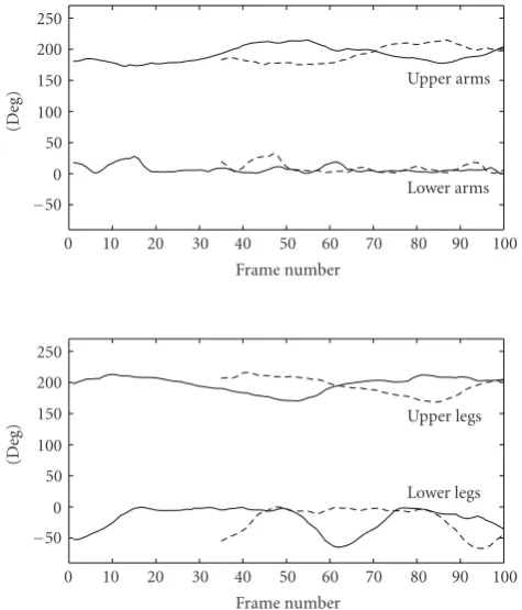
Figure 15: Estimated motion parameters. The top and bottom boxes show the plots of arm and leg pose parameters, respectively (solid lines: right limbs; dashed lines: left limbs).
incorporating the information into the prediction stage. That is, we predict the pose of an occluded limb using the pose pa-rameters of its visible counterpart a half-period prior to the current frame. The initial prediction is adjusted by the im-age measurement. This constraint is far less restrictive than the motion priors employed in [32] or the learned motion model in [10], but we found that it contributes significantly to tracking performance.
0 27
9 36
18 45
Figure16: Tracked walking sequence with very low frame rate.
5.4. Experiments
We have applied the proposed method to many side-view walking sequences; one tracked sequence is shown in Figure 14. We used only about 600 particles for each frame; nevertheless, the result shows very good fitting of the body parts.Figure 15shows the plots of the estimated pose param-eters of the arms and legs. The plots for the left limbs (dashed lines) show only the portion after the half-period prediction is engaged. The plots for the upper limbs generally exhibit more apparent periodicity.
We tested our algorithm on a low frame rate color video; the result is shown inFigure 16. The frame rate is about 15 frames per second, and about 730 particles were used for tracking. We found that tracking is less stable for this se-quence than for the first sese-quence (about 60 frames per sec-ond), although the latter has color information.
Figure 17shows an outdoor walking sequence in which the frame rate is slightly lower than in the previous sequence. We have applied the joint angle symmetry constraints ex-plained in the previous section. While these constraints are restrictive in that they are only applicable to standard walk-ing motion, we found that they effectively limit the parame-ter space, making the tracking much more stable.
0 40
8 48
16 56
24 64
32 72
Figure17: Outdoor walking sequence and tracked motion.
In all of the experiments, the number of particles was around 800 or less. Meanwhile [10,31] reported using 4000 and 5000 particles, respectively, for successful tracking of similar type of walking sequences. We have observed that in-creasing the number of particles did not have much effect when we used more than 800 particles. This verifies the effi -ciency of the approach against other particle-based tracking methods.
6. SUMMARY
We have presented a method of tracking and estimating ob-ject motion using particle propagation and the 3D model of the object. The measurement update is carried out by particle branching according to weights computed by shape-encoded filtering, and the shape constraint provides an ability to es-timate the motion and model parameters. Time update is handled by minimizing the prediction error and adaptive dif-fusion, which contribute to global stability and effectiveness of tracking. More complete analysis and possible
improve-ments would be desirable to ensure global optimization of model or “inertial” parameters. We used very simple models of the head and facial features to generate the shape operators for tracking. Since we need to compute the inverse camera projection for every pixel in the range of the shape operator, constructing the shape operator is highly time-consuming. As shown inSection 2, simple parameterization of the ob-ject surface and feature curves facilitates the construction of the shape operator. The measure helps to reduce computa-tion, and we have obtained satisfactory results. Nevertheless, a more sophisticated parameterization would be desirable to achieve better pose and shape estimation. Figure 10shows another example in which local feature motion is tracked in addition to global object motion; the motions of the irises and upper eyelids are more carefully tracked, so that squint-ing and gaze are recognized. The recognition of facial ex-pression is a possible application of the proposed method. We have also applied the proposed method to the human body tracking problem. The human body model consists of head, torso, and limbs approximated by ellipsoids and trun-cated cones, and body pose is parameterized by joint angles. Other than boundary gradient information, between-frame appearance is computed by using the 3D surface model and provides another image measurement. We dealt with unob-servability due to occlusions of limbs by exploiting the joint motion and symmetry constraints, and found that these nat-ural dynamic constraints contribute to reliable tracking of human walking. We have verified that the method is able to efficiently track walking human in real-life video, using significantly fewer particles than other state-of-the-art ap-proaches.
REFERENCES
[1] H. Moon, R. Chellappa, and A. Rosenfeld, “Optimal edge-based shape detection,”IEEE Transactions on Image Processing, vol. 11, no. 11, pp. 1209–1227, 2002.
[2] A. Azarbayejani and A. P. Pentland, “Recursive estimation of motion, structure, and focal length,”IEEE Transactions on Pat-tern Analysis and Machine Intelligence, vol. 17, no. 6, pp. 562– 575, 1995.
[3] T. J. Broida, S. Chandrashekhar, and R. Chellappa, “Recursive 3-D motion estimation from a monocular image sequence,”
IEEE Transactions on Aerospace and Electronic Systems, vol. 26, no. 4, pp. 639–656, 1990.
[4] G. Kitagawa, “Monte Carlo filter and smoother for non-Gaussian nonlinear state space models,”Journal of Computa-tional and Graphical Statistics, vol. 5, no. 1, pp. 1–25, 1996. [5] J. Liu and R. Chen, “Sequential Monte Carlo methods for
dy-namic systems,”Journal of the American Statistical Association, vol. 93, no. 443, pp. 1032–1044, 1998.
[6] M. Isard and A. Blake, “CONDENSATION—conditional den-sity propagation for visual tracking,”International Journal of Computer Vision, vol. 29, no. 1, pp. 5–28, 1998.
[7] J. Deutscher, A. Blake, and I. Reid, “Articulated body motion capture by annealed particle filtering,” inProceedings of IEEE Computer Society Conference on Computer Vision and Pattern Recognition (CVPR ’00), vol. 2, pp. 126–133, Hilton Head Is-land, SC, USA, June 2000.
IEEE International Conference on Computer Vision (ICCV ’99), vol. 2, pp. 1068–1075, Kerkyra, Greece, September 1999. [9] B. Li and R. Chellappa, “Simultaneous tracking and
verifica-tion via sequential Monte Carlo method,” in Proceedings of IEEE Computer Society Conference on Computer Vision and Pattern Recognition (CVPR ’00), vol. 2, pp. 110–117, Hilton Head Island, SC, USA, June 2000.
[10] H. Sidenbladh, M. J. Black, and D. J. Fleet, “Stochastic track-ing of 3D human figures ustrack-ing 2D image motion,” in Proceed-ings of the 6th European Conference on Computer Vision (ECCV ’00), Dublin, Ireland, June-July 2000.
[11] M. Zakai, “On the optimal filtering of diffusion processes,”
Zeitschrift f¨ur Wahrscheinlichkeitstheorie und Verwandte Gebi-ete, vol. 11, no. 3, pp. 230–243, 1969.
[12] Z. S. Haddad and S. R. Simanca, “Filtering image records using wavelets and the Zakai equation,”IEEE Transactions on Pattern Analysis and Machine Intelligence, vol. 17, no. 11, pp. 1069– 1078, 1995.
[13] D. Crisan, J. Gaines, and T. Lyons, “Convergence of a branch-ing particle method to the solution of the Zakai equation,”
SIAM Journal on Applied Mathematics, vol. 58, no. 5, pp. 1568– 1590, 1998.
[14] D. Crisan and M. Grunwald, “Large deviation comparison of branching algorithm versus resampling algorithms: applica-tion to discrete time stochastic filtering,”Tech. Rep. 9, Cam-bridge University Statistical Laboratory, CamCam-bridge, England, 1999.
[15] M. J. Black and A. D. Jepson, “Eigen tracking: robust match-ing and trackmatch-ing of articulated objects usmatch-ing a view-based rep-resentation,”International Journal of Computer Vision, vol. 26, no. 1, pp. 63–84, 1998.
[16] A. J. Lipton, H. Fujiyoshi, and R. S. Patil, “Moving target clas-sification and tracking from real time video,” inProceedings of the 4th IEEE Workshop on Applications of Computer Vision (WACV ’98), pp. 8–14, Princeton, NJ, USA, October 1998. [17] K. Toyama and A. Blake, “Probabilistic tracking in a metric
space,” inProceedings of the 8th IEEE International Conference on Computer Vision (ICCV ’01), Vancouver, BC, Canada, July 2001.
[18] D. B. Gennery, “Visual tracking of known three-dimensional objects,”International Journal of Computer Vision, vol. 7, no. 3, pp. 243–270, 1992.
[19] D. DeCarlo and D. Metaxas, “Optical flow constraints on de-formable models with applications to face tracking,” Interna-tional Journal of Computer Vision, vol. 38, no. 2, pp. 99–127, 2000.
[20] D. Cremers, “Dynamical statistical shape priors for level set-based tracking,”IEEE Transactions on Pattern Analysis and Ma-chine Intelligence, vol. 28, no. 8, pp. 1262–1273, 2006. [21] O. Chomat and J. L. Crowley, “Probabilistic recognition of
activity using local appearance,” in Proceedings of the IEEE Computer Society Conference on Computer Vision and Pattern Recognition (CVPR ’99), vol. 2, pp. 104–109, Fort Collins, Colo, USA, June 1999.
[22] A. Bensoussan,Stochastic Control of Partially Observable Sys-tems, Cambridge University Press, Cambridge, UK, 1992. [23] L. Ljung, “Asymptotic behaviour of the extended Kalman filter
as a parameter estimator for linear systems,”IEEE Transactions on Automatic Control, vol. 24, no. 1, pp. 36–50, 1979. [24] M. La Cascia, S. Sclaroff, and V. Athitsos, “Fast, reliable head
tracking under varying illumination: an approach based on registration of texture-mapped 3D models,”IEEE Transactions on Pattern Analysis and Machine Intelligence, vol. 22, no. 4, pp. 322–336, 2000.
[25] J. Xiao, T. Moriyama, T. Kanade, and J. Cohn, “Robust full-motion recovery of head by dynamic templates and re-registration techniques,”International Journal of Imaging Sys-tems and Technology, vol. 13, no. 1, pp. 85–94, 2003.
[26] L. Sigal, S. Bhatia, S. Roth, M. J. Black, and M. Isard, “Track-ing loose-limbed people,” inProceedings of IEEE Computer So-ciety Conference on Computer Vision and Pattern Recognition (CVPR ’04), vol. 1, pp. 421–428, Washington, DC, USA, June-July 2004.
[27] A. Agarwal and B. Triggs, “Recovering 3D human pose from monocular images,”IEEE Transactions on Pattern Analysis and Machine Intelligence, vol. 28, no. 1, pp. 44–58, 2006.
[28] C. Curio and M. A. Giese, “Combining view-based and model-based tracking of articulated human movements,” in Pro-ceedings of IEEE Workshop on Motion and Video Computing (WACV/MOTIONS ’05), vol. 2, pp. 261–268, Breckenridge, Colo, USA, January 2005.
[29] D. Ramanan, D. A. Forsyth, and A. Zisserman, “Tracking peo-ple by learning their appearance,”IEEE Transactions on Pat-tern Analysis and Machine Intelligence, vol. 29, no. 1, pp. 65–81, 2007.
[30] M. W. Lee and I. Cohen, “Proposal maps driven MCMC for estimating human body pose in static images,” inProceedings of IEEE Computer Society Conference on Computer Vision and Pattern Recognition (CVPR ’04), vol. 2, pp. 334–341, Washing-ton, DC, USA, June-July 2004.
[31] J. Deutscher, B. North, B. Bascle, and A. Blake, “Tracking through singularities and discontinuities by random sam-pling,” in Proceedings of the 7th IEEE International Confer-ence on Computer Vision (ICCV ’99), vol. 2, pp. 1144–1149, Kerkyra, Greece, September 1999.