Instrumental Variable and Propensity Score Methods for Bias Adjustment in Non-Linear Models

University of Pennsylvania

ScholarlyCommons

Publicly Accessible Penn Dissertations

1-1-2015

Instrumental Variable and Propensity Score

Methods for Bias Adjustment in Non-Linear

Models

Fei Wan

University of Pennsylvania, [email protected]

Follow this and additional works at:

http://repository.upenn.edu/edissertations

Part of the

Biostatistics Commons

This paper is posted at ScholarlyCommons.http://repository.upenn.edu/edissertations/2087

Recommended Citation

Wan, Fei, "Instrumental Variable and Propensity Score Methods for Bias Adjustment in Non-Linear Models" (2015).Publicly Accessible Penn Dissertations. 2087.

Instrumental Variable and Propensity Score Methods for Bias Adjustment

in Non-Linear Models

Abstract

Unmeasured confounding is a common concern when clinical and health services researchers attempt to

estimate a treatment effect using observational data or randomized studies with non-perfect compliance. To

address this concern, instrumental variable (IV) methods, such as two-stage predictor substitution (2SPS)

and two-stage residual inclusion (2SRI), have been widely adopted. In many clinical studies of binary and

survival outcomes, 2SRI has been accepted as the method of choice over 2SPS but a compelling theoretical

rationale has not been postulated.

First, We directly compare the bias in the causal hazard ratio estimated by these two IV methods. Under the

potential outcome and principal stratification framework, we derive closed form solutions for asymptotic bias

in estimating the causal hazard ratio among compliers for both the 2SPS and 2SRI methods by assuming

survival time follows the Weibull distribution with random censoring. When there is no unmeasured

confounding and no always takers, our analytic results show that 2SRI is generally asymptotically unbiased

but 2SPS is not. However, when there is substantial unmeasured confounding, 2SPS performs better than

2SRI with respect to bias under certain scenarios. We use extensive simulation studies to confirm the analytic

results from our closed-form solutions. We apply these two methods to prostate cancer treatment data from

SEER-Medicare and compare these 2SRI and 2SPS estimates to results from two published randomized trials.

Next, we propose a novel two-stage structural modeling framework to understanding the bias in estimating

the conditional treatment effect for 2SPS and 2SRI when the outcome is binary, count or time to event. Under

this framework, we demonstrate that the bias in 2SPS and 2SRI estimators can be reframed to mirror the

problem of omitted variables in non-linear models. We demonstrate that only when the influence of the

unmeasured covariates on the treatment is proportional to their effect on the outcome that 2SRI estimates are

generally unbiased for logit and Cox models. We also propose a novel dissimilarity metric to quantify the

difference in these effects and demonstrate that with increasing dissimilarity, the bias of 2SRI increases in

magnitude. We investigate these methods using simulation studies and data from an observational study of

perinatal care for premature infants.

Last, we extend Heller and Venkatraman's covariate adjusted conditional log rank test by using the propensity

score method. We introduce the propensity score to balance the distribution of covariates among treatment

groups and reduce the dimensionality of covariates to fit the conditional log rank test. We perform the

simulation to assess the performance of this new method and covariates adjusted Cox model and score test.

Degree Type

Dissertation

Degree Name

Doctor of Philosophy (PhD)

Graduate Group

First Advisor

Nandita Mitra

Second Advisor

Dylan Small

Keywords

bias, causal inference, Instrumental variable, observational studies, propensity score, survival analysis

Subject Categories

INSTRUMENTAL VARIABLE AND PROPENSITY SCORE METHODS FOR BIAS ADJUSTMENT IN NON-LINEAR MODELS

Fei Wan A DISSERTATION

in

Epidemiology and Biostatistics

Presented to the Faculties of the University of Pennsylvania in

Partial Fulfillment of the Requirements for the Degree of Doctor of Philosophy

2015

Supervisor of Dissertation Co-Supervisor of Dissertation

Nandita Mitra Dylan Small

Associate Professor of Biostatistics Professor of Statistics

Graduate Group Chairperson

John H. Holmes, Professor of Medical Informatics in Epidemiology

Dissertation Committee

INSTRUMENTAL VARIABLE AND PROPENSITY SCORE METHODS FOR BIAS ADJUSTMENT IN NON-LINEAR MODELS

© COPYRIGHT 2015

Fei Wan

This work is licensed under the Creative Commons Attribution NonCommercial-ShareAlike 3.0 License

To view a copy of this license, visit

ACKNOWLEDGEMENT

I would like to gratefully and sincerely thank two of my advisors: Drs. Nandita Mitra and Dylan Small, for their advising and guidance, understanding, and patience through every stage of my dissertation research. Without their generous support, it is unlikely for me to complete this work. I would like to express my special thanks to Dr. Mitra for her mentorship for almost 10 years. Only under her encouragement and generous help, I am able to fulfill my lifetime dream of completing a Ph.D degree at Penn.

I would like to express my gratitude to my dissertation committee members for their collaboration and flexibility with my dissertation meetings. I need to thank Dr. Justin Bekelman for his time and efforts on my first methodology paper. I like to thank Dr. Sharon Xie for her generous advices on my questions on survival models. I need further thank all the faculties and fellow students of Penn biostatistics program. Studying at Penn is truly unique educational experience for me.

ABSTRACT

INSTRUMENTAL VARIABLE AND PROPENSITY SCORE METHODS FOR BIAS ADJUSTMENT IN NON-LINEAR MODELS

Fei Wan Nandita Mitra

Dylan Small

Unmeasured confounding is a common concern when clinical and health services researchers attempt to estimate a treatment effect using observational data or randomized studies with non-perfect compliance. To address this concern, instrumental variable (IV) methods, such as two-stage predictor substitution (2SPS) and two-stage residual inclusion (2SRI), have been widely adopted. In many clinical studies of binary and survival outcomes, 2SRI has been accepted as the method of choice over 2SPS but a compelling theoretical rationale has not been postulated.

effect on the outcome that 2SRI estimates are generally unbiased for logit and Cox models. We also propose a novel dissimilarity metric to quantify the difference in these effects and demonstrate that with increasing dissimilarity, the bias of 2SRI increases in magnitude. We investigate these meth-ods using simulation studies and data from an observational study of perinatal care for premature infants.

TABLE OF CONTENTS

ACKNOWLEDGEMENT . . . iii

ABSTRACT . . . iv

LIST OF TABLES . . . viii

LIST OF ILLUSTRATIONS . . . x

CHAPTER 1 : INTRODUCTION . . . 1

CHAPTER 2 : BIAS IN TWO STAGE INSTRUMENTAL VARIABLE METHODS . . . 5

2.1 Introduction . . . 5

2.2 Notation, Assumptions, Compliance Categories, and Model . . . 6

2.3 Two Stage Predictor Substitution(2SPS)Method . . . 9

2.4 Two Stage Residual Inclusion(2SRI)Method . . . 14

2.5 Simulation . . . 18

2.6 Seer-Medicare Prostate Cancer Study . . . 20

2.7 Discussion . . . 22

2.8 Appendix . . . 23

CHAPTER 3 : A GENERAL FRAMEWORK FOR ASSESSING BIAS IN TWO-STAGE INSTRU -MENTALVARIABLEMODELS . . . 49

3.1 Introduction . . . 49

3.2 Notations, Assumptions, and Framework . . . 51

3.3 Bias analysis . . . 55

3.4 Simulation . . . 64

3.5 Discussion . . . 66

3.6 Appendix . . . 67

4.1 Introduction . . . 88

4.2 Test Statistic . . . 90

4.3 Simulation study . . . 94

4.4 Discussion . . . 95

CHAPTER 5 : DISCUSSION. . . 99

LIST OF TABLES

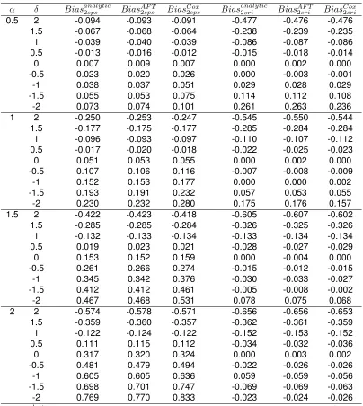
TABLE 2.1 : Bias in estimating log causal hazard ratio parameter (ρa = 0, ρc = 0.5, ρr=

0.8, θ1

c = 3.33, θ

0

c = 1.67) . . . 47

LIST OF ILLUSTRATIONS

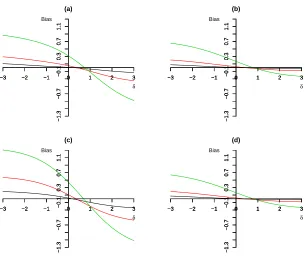
FIGURE 2.1 : Plot of bias against magnitude of unmeasured confounding∆using 2SPS method:(a)P(R= 1) = 0.8,ρa = 0,ρc = 0.5,θ1c = 3.33,θ

0

c = 1.67.(b)P(R=

1) = 0.8,ρa = 0,ρc = 0.8,θ1c = 3.33,θ

0

c = 1.67.(c)P(R= 1) = 0.8,ρa= 0,

ρc = 0.5, θc1 = 33.3, θc0 = 16.7. (d) P(R = 1) = 0.5, ρa = 0, ρc = 0.8,

θ1

c = 3.33, θc0 = 1.67. The different colour of solid line corresponds to

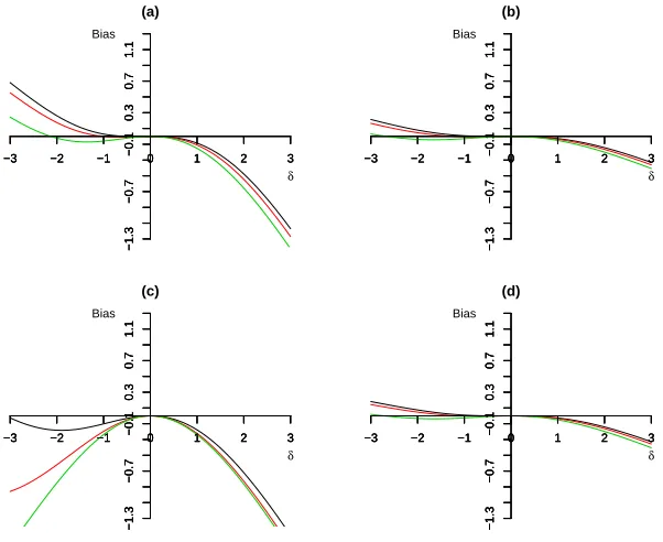
different shape parameter: black (α= 0.5),red (α= 1),and green (α= 2). . 45 FIGURE 2.2 : Plot of bias against magnitude of unmeasured confounding∆using 2SRI

method:(a)P(R= 1) = 0.8,ρa = 0,ρc = 0.5,θ1c = 3.33,θc0= 1.67.(b)P(R=

1) = 0.8,ρa = 0,ρc = 0.8,θ1c = 3.33,θc0= 1.67.(c)P(R= 1) = 0.8,ρa= 0,

ρc = 0.5, θc1 = 33.3, θc0 = 16.7. (d) P(R = 1) = 0.5, ρa = 0, ρc = 0.8,

θ1

c = 3.33, θc0 = 1.67. The different colour of solid line corresponds to

different shape parameter: black (α= 0.5),red (α= 1),and green (α= 2). . 46 FIGURE 2.3 : Absolute bias in estimating log causal hazard ratio using two stage IV

meth-ods (X-axis is the magnitude of confounding∆, Y-axis is the absolute bias). For 2SRI method or 2SPS method, the biases computed for each of 1458 possible scenarios were grouped by the magnitude of shape parameterα

(decreasing hazard for α = 0.5, constant hazard forα= 1, and increas-ing hazard forα = 2) and the magnitude of confounding∆(larger values represent lager confounding effects and 0 represents no confounding). . . 46 FIGURE 2.4 : Mean square error in estimating log causal hazard ratio using two stage IV

methods (X-axis is the magnitude of confounding ∆, Y-axis is the Mean Square Error).For 2SRI method or 2SPS method, the mean square error computed for each of 1458 possible scenarios were grouped by the magni-tude of shape parameterα(decreasing hazard forα= 0.5, constant hazard forα= 1, and increasing hazard forα= 2) and the magnitude of confound-ing∆(larger values represent lager confounding effects and 0 represents no confounding). . . 48 FIGURE 3.1 : Decomposingβ3into two orthogonal components . . . 80

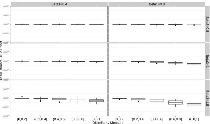
FIGURE 3.2 : Boxplot of 2SRI Poisson model estimates when treatment effect is nonzero.

β1 is treatment effect; β3is effect of unmeasured covariates on outcome.

Bias is the difference between estimates and true treatment effect . . . 80 FIGURE 3.3 : Boxplot of 2SRI logistic model estimates when treatment effect is nonzero.

β1 is treatment effect; β3is effect of unmeasured covariates on outcome.

Bias is the difference between estimates and true treatment effect. . . 81 FIGURE 3.4 : Boxplot of 2SRI Cox model estimates when treatment effect is nonzero. β1

is treatment effect;β3is effect of unmeasured covariates on outcome. Bias

is the difference between estimates and true treatment effect. Red colored box is for low level effect of unmeasured covariates (β3 = 0.5). Green

colored box is for medium level effect of unmeasured covariates (β3 = 1).

Blue colored box is for high level effect of unmeasured covariates (β3= 1.5) 82

FIGURE 3.5 : Boxplot of 2SRI Cox model estimates when treatment effect is nonzero. β1

is treatment effect;β3is effect of unmeasured covariates on outcome. Bias

is the difference between estimates and true treatment effect.Red colored box is for smaller size of treatment effect (β1= 0.4). Green colored box is

for medium level effect of unmeasured covariates (β1= 0.8) . . . 83

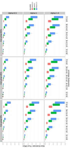
FIGURE 3.7 : Boxplot of 2SRI Poisson model estimates when treatment effect is zero. Color red- effects of unmeasured covariates are low (β3 = 0.5); Color

green-effects of unmeasured covariates are medium (β3 = 1); Color

blue-effects of unmeasured covariates are high (β3= 1.5) . . . 85

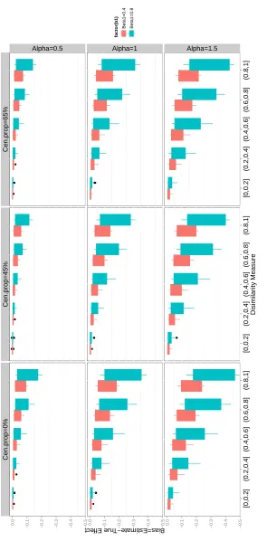
FIGURE 3.8 : Boxplot of 2SRI logistic model estimates when treatment effect is zero. Color red- effects of unmeasured covariates are low (β3 = 0.5); Color

green-effects of unmeasured covariates are medium (β3 = 1); Color

blue-effects of unmeasured covariates are high (β3= 1.5) . . . 86

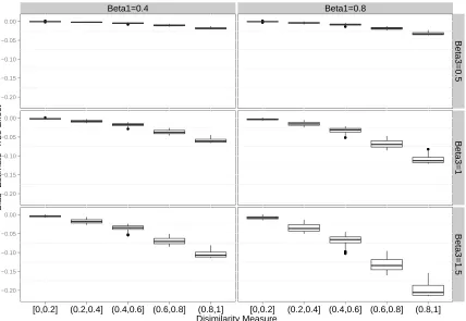
FIGURE 3.9 : Boxplot of 2SRI Cox model estimates when treatment effect is zero. Color red- effects of unmeasured covariates are low (β3 = 0.5); Color

green-effects of unmeasured covariates are medium (β3= 1); Color blue-effects

of unmeasured covariates are high (β3= 1.5) . . . 87

FIGURE 4.1 : Boxplot of type I error rates for unadjusted log rank test, score test based on Cox proportional hazard model, robust score tests (lin and Wei, Kong and Slud), and propensity score adjusted log rank test . . . 97 FIGURE 4.2 : Scatter plots of the power for the propensity score adjusted log rank test

CHAPTER 1

I

Evaluating the effectiveness of treatment and identifying the causal relationships between exposure and disease are critical objectives for clinical and health services researchers. The casual effects of a treatment can be rigorously defined under the potential outcomes framework (Holland, 1986; Rubin, 2005). Consider a case of a two arm trial that involves one active treatment and a control of no treatment. Let Zi denote binary treatment status variable, whereZi = 1if subject i takes

the active treatment and Zi = 0 if subjectireceives the control. YiZ=1 is the potential outcome,

on a continuous scale, when subject i receives the active treatment and YZ=0

i is the potential

outcome if subject i actually takes the control. The simple treatment effect for subject i is the difference between the two potential outcomes, defined asYZ=1

i −YiZ=0. Clearly, only one potential

outcome can be observed and the other one is often referred as “counter-factual” and written as

Yi = ZiYiZ=1 + (1−Zi)YiZ=0. Therefore, it is not possible to identify the casual effect for an

individual because of this missing data issue (Rubin, 2005). However, the average casual effect

E(YZ=1

i −YiZ=0)for the population is identifiable from the data if certain assumptions are met.

Assume a binary treatmentZis randomized in the population and every subject complies with their assignment. Under the exchange-ability and consistency assumptions (Hernán and Robins, 2006a; Robins J.M. and Brumback, 2000), population average causal effect of treatment is consistently estimated by the difference between two group means,

E(YZ=1

i −Y

Z=0

i ) =E(Yi|Zi= 1)−E(Yi|Zi = 0)

= ¯Y1−Y¯0

may exist prognostic factors that influence patients’ compliance with treatment assignment. Thus, the estimator of treatment effect is biased when confounding factors are not fully measured and controlled for (Hernán and Hernández-Díaz, 2012). Alternatively, intention-to-treat analysis (ITT) is a widely accepted simple approach to non-compliance and subjects are analysed according to ran-domization scheme regardless of treatment actually received. Although the integrity of randomiza-tion is retained, ITT tends to underestimate treatment effects, and it measures the causal effects of treatment assignment, instead of effectiveness of treatment (Hernán and Hernández-Díaz, 2012). Besides non-compliance problem, RCTs are subject to many other limitations, such as lack of gen-eralizability, high cost, lengthy study period, ethic concerns, and difficulty in studying rare diseases, etc (Nallamothu and Hayward, 2008). When a RCT is not feasible, non-randomized observational studies are commonly used to examine the effectiveness of treatment or therapy in routine clini-cal practice. Compared to RCTs, well designed observational studies can provide more realistic results. Confounding, whether observed or not, is also the main problem of estimating the causal effects in observational studies. The traditional statistical methods, such as stratification, matching, multiple regression, and propensity score, have been used to reduce bias (Martens et al., 2006). These methods are valid under the assumption of no unmeasured confounding variables. In many cases, however, this assumption is very likely to be violated.

An alternative method that could potentially control for both measured and unmeasured confound-ing variables is the instrumental variable (IV) method. An IV has the followconfound-ing properties: (i) IV either correlates with or has causal effects on treatment or exposure; (ii) IV has no direct effects on outcome except its indirect effects through either treatment or exposure. (iii) there is no un-measured confounding for the association between IV and outcome variable (Angrist, Imbens, and Rubin, 1996; Hernán and Robins, 2006b). Random assignment scheme in RCTs is an example of IV.

grow-ing. Terza, Basu, and Rathouz, 2008 made the extension of two IV based approaches, two-stage residual inclusion (2SRI) and two-stage predictor substitution (2SPS), to correcting for endogeneity bias in non-linear models for both binary and time to event outcome. When two IV methods are compared for their performance in estimating the conditional odds ratio or hazard ratio (on unmea-sured confounding), they conclude that only 2SRI method produces consistent estimates. This finding rapidly increases the use of 2SRI method to control for unmeasured confounding in medical research (Hadley et al., 2010; Tan et al., 2012).

Under the frame work of potential outcomes, Angrist, Imbens, and Rubin, 1996 divided the subjects accordingly into four principal strata: 1) compliers, who always follow treatment assignment; 2) always takers, who always take the treatment; 3) defiers, who always take the opposite to treatment assignment; and 4) never takers, who never take treatment. They proved that IV estimator of two-stage least squares method consistently estimates a local averaged treatment effects (LATE) among compliers under five assumptions. The details of assumptions are discussed in Chapter 2. Under the same framework of potential outcomes and principal stratification, Cai, Small, and Ten Have, 2011 found analytically and by simulation that both 2SRI and 2SPS logistic regressions generated biased estimate of LATE among compliers. In chapter 2, under the same potential outcome and principal stratification framework, we derive closed form solutions for asymptotic bias in estimating the causal hazard ratio among compliers for both the 2SPS and 2SRI methods by assuming survival time follows the Weibull distribution with random censoring.

In chapter 3, we further assess the performance of 2 stage IV methods in estimating the conditional treatment effect given observed and unobserved covariates. For this purpose, we propose a novel two-stage structural modeling framework to accommodate one endogenous treatment variable and multiple unobserved covariates. This new framework is more relevant to clinical settings. Utilizing this framework, we demonstrate that the bias in 2SPS and 2SRI estimators can be reframed to mirror the problem of omitted variables in non-linear models. We demonstrate that only when the influence of the unmeasured covariates on the treatment is proportional to their effect on the outcome that 2SRI estimates are generally unbiased for logit and Cox models.

CHAPTER 2

B

2.1. Introduction

Evaluating the effectiveness of treatment and identifying the causal relationship between exposure and disease are critical objectives for clinical and health services researchers. Confounding is often a concern when analyzing non-randomized observational studies and even randomized studies with non-compliance (Hernán and Robins, 2006b). Instrumental variable (IV) methods are increasingly being used in clinical comparative effectiveness studies to potentially control for both measured and unmeasured confounding. Angrist, Imbens, and Rubin, 1996 defined the IV for causal effects of treatment on outcome to be a variable satisfying the following five assumptions: i)The potential outcomes on one subject are unrelated with the particular assignment of treatment to the other subjects; ii) IV is randomly (or ignorably) assigned; iii) Any effect of IV on the outcome must be mediated by treatment received(the exclusion restriction);iv) IV has nonzero effect on treatment received; v) There are no defiers. (for details see section 2.2)

In a recent clinical study, we were interested in comparing the effectiveness of two treatments for prostate cancer in elderly men using SEER-Medicare, a large national observational database. Specifically, we planned to use IV methods to estimate the effect of the addition of external beam radiation therapy (EBRT) to androgen suppression therapy (ADT) in improving overall survival in men with locally advanced prostate cancer. We considered a commonly used IV in health services research: local area treatment patterns defined by the percentage of active treatment in hospital referral regions (HRR). This IV has been shown to capture regionally distinct structural variation in care (Bekelman et al., 2015). Such variation is not fully explained by patient characteristics. Further, this IV varies across HRRs and is strongly associated with treatment assignment. Finally, it is balanced across important observed prognostic factors. Although there is an extensive literature on the importance of choosing an appropriate instrument, less attention has been paid to using the appropriate modeling approach once an IV is selected.

and Ten Have, 2011; Terza, Basu, and Rathouz, 2008).These methods have been used to cor-rect for bias due to endogeneity in non-linear models for both binary and time-to-event outcomes. Among these two IV approaches, 2SRI was shown to consistently estimate a conditional causal parameter under certain assumptions (Terza, Basu, and Rathouz, 2008) and has been adopted as the method of choice in clinical research studies involving survival outcomes(Gore et al., 2010; Hadley et al., 2010; Tan et al., 2012). The conditional causal parameter that Terza, Basu, and Rathouz, 2008 consider is only identified by making homogeneity assumptions that go beyond the five assumptions for a valid IV defined in the first paragraph. Angrist, Imbens, and Rubin, 1996 showed that under these five assumptions for a valid IV, the only treatment effect that is identified is the average treatment effect for the compliers, where the the compliers are the subjects who would take the treatment if encouraged to do so by the IV but would not take the treatment if not encour-aged by the IV; this is called the local average treatment effect (LATE).In the context of a binary outcome, Cai, Small, and Ten Have, 2011 demonstrated that both the 2SRI and 2SPS methods generated biased estimates of LATE among compliers for binary outcome. In this paper, we focus on the properties of 2SPS and 2SRI as estimators of the LATE for time-to-event data.

Despite the fact that there is growing interest in applying two stage IV methods to time-to-event data, little is known about the potential bias of using such methods to estimate LATE among compliers. We derive closed form expressions of the bias and conduct extensive simulations to quantify this bias. We then apply both of the two-stage IV methods to our prostate cancer treatment data and compare them to the results from two published randomized clinical trials (Warde et al., 2011; Widmark et al., 2009)

2.2. Notation, Assumptions, Compliance Categories, and Model

2.2.1. Notation

area rate (above median) of adding EBRT to ADT and 0 represents a low local area rate (below the median) of adding EBRT to ADT. Theith elementRi = 1implies that subjecti is encouraged to

receive the active treatment, whereasRi= 0indicates that subjectiis not encouraged to receive

the active treatment. LetZR

be an N-dimensional vector of potential treatment received givenR, andith elementZiR=1 indicates that subjectireceives the active treatment andZ

R

i =0 means that

subjectireceives the control underR.

Similarly, we defineTR,Z to be an N-dimensional vector of potential survival time underRandZ, and ith element TiR,Z is the potential survival time for subject i underR and Z. Let L

R,Z

to be an N-dimensional vector of potential censoring time under RandZ, andith elementLR,Zi is the

potential censoring time for subjectiunderRandZ.

We defineYR,Z=min_{TR,Z, LR,Z}, the elementwise minimum of potential censoring and survival times,to be an N-dimensional vector of potential observed follow up time underR andZ, andith element YiR,Z represents the potential follow up time for subject i under R andZ. Let δ

R,Z

i =

I_{TiR,Z ≤ C R,Z

i }indicates whether subject iis observed to terminate by failure (δ R,Z

i = 1) or by

censoring (δiR,Z=0) givenRandZ. The vectorXi represents measured confounding variables for

subjecti.

2.2.2. Assumptions

The main assumptions we will make for causal modeling are the five assumptions made by Angrist et al. (Angrist, Imbens, and Rubin, 1996), and a random censoring assumption for the survival setting.

1) Stable Unit Treatment Value Assumption (SUTVA)(Rubin, 1986, 1990) a. ifRi=R0i, thenZ

R

i =Z

R0

i

b. ifRi=R0iandZi=Zi0, thenY R,Z

i =Y

R0,Z0

i

The SUTVA assumption says that the potential outcomes for subjectiare not related with the treat-ment status of other subjects such that we can writeZiR,Y

R,Z

i ,T

R,Z

i ,L

R,Z

i ,δ

R,Z

i asZ

Ri

i ,Y

Ri,Zi

i ,T

Ri,Zi

i ,L

Ri,Zi

i ,

δRi,Zi

i respectively. The SUTVA assumption also implies the assumption of consistency, such that

2) Independence of the instrumentR(Abadie, 2003):

Conditional on a vector of confounders X, the random vector (YR,Z, TR,Z, LR,Z, ZR) is indepen-dent of R. In a randomized trial whereR is the IV, the independence assumption holds without conditioning onX.

3) Exclusion Restriction

∀Z, R, andR0_{, we have:}

TR,Z _{= T}R0,Z

, LR,Z _{= L}R0,Z

, YR,Z _{= Y}R0,Z

, This assumption implies that any effect of IV on potential outcomes must be through its effect on treatment actually received. Thus, we can write

TiR,Z,L R,Z

i ,Y

R,Z

i asT

Zi

i ,L

Zi

i ,Y

Zi

i by combining the exclusion restriction and SUTVA assumptions.

4) Non-zero Average Causal Effect ofRonZ E[Z1

i −Z

0

i]6= 0

This assumption means the IV is correlated with treatment received. 5) Monotonicity (Imbens and Angrist, 1994)

Z1

i ≥Zi0,∀i∈N

This assumption rules out the existence of defiers. No subject always does the opposite of the treatment assigned.

6) Independent censoring

The distribution of potential survival timeTR,Z is independent of the distribution of potential cen-soring timeLR,Z.

2.2.3. Compliance Categories

Under the framework of principal stratification and potential outcomes (Angrist, Imbens, and Rubin, 1996; Rubin, 2005), subjects in a two-arm randomized trial can be categorized into 4 principal strata: Always takers (AT) are subjects who always take the treatment regardless of assignments (Z1 _{= 1, Z}0_{= 1); Compliers (C) are subjects who comply with their assignments(Z}1 _{= 1, Z}0 _{= 0);}

Never takers (NT) are the subjects who never take the treatment no matter which group they are assigned to(Z1 _{= 0, Z}0 _{= 0}

2.2.4. Model

We first define the probability of receiving the treatmentP r(R= 1) =r, the probability of being a always taker P r(AT) = ρa, and the probability of being a complier P r(C) = ρc. We also define

the probability of being a defierP r(D) =ρd, but under the monotonicity assumption, there are no

defiers so thatρd= 0. Hence, the probability of being a never takerP r(N T)is equal to1−ρa−ρc.

We assume both potential censoring time and potential survival time follow the Weibull distribution with the same shape parameterα. The potential censoring time for the subjects in each principal strata followsW eibull(α, λ), and we define the parameters of the probability distribution of potential survival time for each principal strata as follows:

T1|AT ∼W eibull(α, θ1at), T

0

|AT ∼W eibull(α, θat0)

T1

|C_∼W eibull(α, θ1

c), T

0

|C_∼W eibull(α, θ0

c)

T1

|N T _∼W eibull(α, θ1

nt), T

0

|N T _∼W eibull(α, θ0

nt)

We also examined scenarios in which different shape parameters α’s are assumed for the po-tential censoring time and the popo-tential survival time. These details are given in Appendix E. The density of Weibull distribution is f(t) = (α/K)(t/K)K−1_exp(

−(t/K)α_{) and the hazard rate}

ish(t) = αK−α_tα−1_{. In the case of Weibull regression with covariatesX,K}−α_{can be}

reparame-terized asexp(βX). The hazard rate for the compliers if treated ish(T1_=t

|C) =αtα−1_(θ1

c)−α. The

hazard rate for the compliers if not treated ish(T0 _=t

|C) = αtα−1_(θ0

c)−α. Hence, the log causal

hazard ratioφfor the compliers is the difference between two log hazard rates:

φ=log[h(T1_=t

|C)]₋log[h(T0_=t

|C)]

=−α(log(θ1c)−log(θ

0

c))

2.3. Two Stage Predictor Substitution(2SPS)Method

P =E(Z|R). In the second stage, a log linear model includingP ,defined as:

log[h(Y|P)] =η+ξP+log(h0(y)), h0(Y) =αyα−1

is fitted to estimate the coefficientξ. This is 2SPS estimator of the log causal hazard ratio. We first derive a closed form expression to the probability limit of the maximal likelihood estimator (M.L.E) ofξ, then take the difference between this probability limit and true log causal parameterφfor the expression of the asymptotic bias of the 2SPS estimator as an estimator of the log causal hazard ratio for compliers.

2.3.1. Probability limit of M.L.E of causal parameter

LetPˆ denote the predicted value from the estimated binary regression model. i.e., Pˆ = ˆE(Z|R). WhenPˆis substituted forP, the second stage Weibull model becomes:

log[λ(Y_|Pˆ)] =η∗+ξ∗Pˆ+log(h∗0(y))

Letξˆ∗_{andξˆdenote the estimators (M.L.E) ofξ}∗_{andξrespectively. As sample sizen}

→ ∞,Pˆ_→P,

ˆ ξ∗ p

−→ξˆ, andξˆ_−→p ξ. Therefore,ξˆ∗ p

−→ξ. To derive closed form expression for the asymptotic bias, we need to re-expressξin terms of parameters specified in Section 2.2 under the principal stratification framework.

Only always takers receive the treatment when assigned to control(R= 0). Both always takers and compliers take the treatment when assigned to treatment(R= 1). Thus, it can be shown that (Cai, Small, and Ten Have, 2011):

p0=E(Z|R= 0) =ρa, p1=E(Z|R= 1) =ρa+ρc

Since P = _{p0, p1} is an one-to-one transformation ofR = {0,1}, we have the following for the

second stage Weibull regression:

log(h(Y|R= 0)) =log(h(Y|P =p0))

and,

log(h(Y|R= 1)) =log(h(Y|P =p1))

=η+ξp1+log(h0(y)) (2.2)

Instead of working with a second stage model involvingP, we can work with a model involvingR

instead. Solving (2.1) and (2.2), we have:

ξ= log(h(Y|R= 1))−log(h(Y|R= 0)) p1−p0

(2.3)

The log linear model includingRassumes two underlying Weibull distributions of the same shape parameterα∗_{,W eibull(α}∗_{, K}

0)andW eibull(α∗, K1), for subjects assigned to control (R= 0) and

treatment (R= 1) respectively. Thus, (2.3) can be expressed as:

ξ= log(K

−α∗

1 )−log(K −α∗

0 )

ρc

, K1−α∗=e

η+ξp1_{, K}−α∗

0 =e

η+ξp0 _(2.4)

It is worth noting that both follow up times of subjects assigned to control, denoted as Y|R = 0, and follow up times of subjects assigned to treatment, denoted asY|R= 1, actually follow mixture distributions consisting of three different Weibull distributions. Details are given in Appendix A. However, the second stage Weibull model of 2SPS method imposes the two Weibull distributions, with the same shape parameterα∗_{but different scale parametersK}

0, K1, upon subjects assigned

to treatment(R = 1) or assigned to control(R = 0) respectively. Thus, the M.L.E of α∗_{, K} 0, K1

are derived by maximizing the likelihood functionLn(α∗, K0, K1)that consists of products of two

Weibull densities:W eibull(α∗_{, K}

0)andW eibull(α∗, K1).

Let αˆ∗ _{denote the M.L.E of α}∗ _{and We set E(}∂log(Ln(α∗,Kˆ0(α∗),Kˆ1(α∗))

∂α∗ ), the expectation of score

equation derived from profile likelihood of α∗_{, equal to 0 and let} f

α∗ _{be the solution. Under the}

assumptions stated in Section 2.2 and consistency of M.L.E, the probability limit of the estimator

ˆ α∗_is

f

α∗_{. Details are given in Appendix C. Once the parameters of the principal strata are defined,} f

α∗ _{can be solved numerically using a root-finding algorithm such as the "bisection" method. Let}

ˆ

determined, the probability limits of the estimatorsKˆ0,Kˆ1can be derived as follows:

f

K0= [

1

P(δ= 1|R= 0)×

{ρaΓ(f

α∗

α + 1)[

1

θ1

at

α +

1

λα]

−αf∗/α

+ρnΓ(f

α∗

α + 1)[

1

θ0

nt

α+

1

λα]

−αf∗/α

+ρcΓ(f

α∗

α + 1)[

1

θ0

cα

+ 1

λα]

−αf∗/α

}]1/αf∗

(2.5)

and,

f

K1= [

1

P(δ= 1|R= 1)×

{ρaΓ( f

α∗

α + 1)[

1

θ1

at

α +

1

λα]

−αf∗/α

+ρnΓ( f

α∗

α + 1)[

1

θ0

nt

α+

1

λα]

−αf∗/α

+ρcΓ( f

α∗

α + 1)[

1

θ1

cα

+ 1

λα]

−αf∗/α

}]1/αf∗

(2.6)

The detailed steps of the derivation of (2.5) and (2.6) are given in Appendix C. By substituting (2.5) and (2.6)

into (2.4), we derive the expression of log causal hazard ratioξas the following:

ξ={log([ 1

P(δ= 1|R= 1)×

{ρaΓ( f

α∗

α + 1)[

1

θ1

at

α +

1

λα]

−αf∗/α

+ρnΓ( f

α∗

α + 1)[

1

θ0

nt

α +

1

λα]

−αf∗/α

+ρcΓ( f

α∗

α + 1)[

1

θ1

c

α+

1

λα]

−αf∗/α

}])−1

−log([ 1

P(δ= 1|R= 0)×

{ρaΓ( f

α∗

α + 1)[

1

θ1

at

α +

1

λα]

−αf∗/α

+ρnΓ( f

α∗

α + 1)[

1

θ0

nt

α +

1

λα]

−αf∗/α

+ρcΓ( f

α∗

α + 1)[

1

θ0

c

α+

1

λα]

−αf∗/α

}])−1}

× 1

ρc

(2.7)

Thus, (2.7) is the closed-form expression of the probability limit of the log causal hazard ratio estimatorξˆ∗from

the 2SPS Weibull model.

2.3.2. Bias analysis

The asymptotic bias of the causal parameterξof the 2SPS Weibull regression model is simply the difference

between the true log causal hazard ratioφand the derived closed form expression ofξ, such that

B2sps=ξ+α(log(θc1)−log(θ

0

We can re-paramterizeθ0ntin (2.8) with one additional parameter∆ =−α(log(θ0nt)−log(θ0c))as the following:

log(θnt0 ) =log(θ

0

c) +

∆

α (2.9)

∆in (2.9) is the log hazard ratio between never takers and compliers given no treatment. It can be interpreted

as the magnitude of the unmeasured confounding because the differences between principal strata are

at-tributable to the unmeasured confounding (Cai, Small, and Ten Have, 2011). When∆ = 0orθ0nt=θ0c,there is

no unmeasured confounding.

We make the following observations about the bias of 2SPS method from (3.11): 1) Whenα = 1and we

treatα∗as a known parameter and fix it at 1, that is the scenario when the survival outcomes of all principal

strata follow exponential distributions and we also fit an exponential model in the second stage instead of

estimating the shape parameter for a more general form of Weibull distribution; 2) Whenρc= 1, every subject

is a complier and (2.8) can be simplified as 1

α∗ −

γ

α −ψ(

α∗

α + 1)

1

α = 0. Then we have αf∗ = α. Setting

ρc = 1,ρa = 0, andρn = 0, (2.8) becomes 0 so that biasB2sps = 0when a randomized controlled trial has

perfect compliance; 3) When there is no causal effect (θ1c = θ0c), all terms in (2.8) cancel out and we have

B2sps = 0; 4) Whenρa = 0andθc0 =θ0n, there is no confounding because there are no always takers and

never takers can’t get treatment so that the confounding can only be attributable to the difference between

never takers and compliers given no treatment(Cai, Small, and Ten Have, 2011). However, (2.8) can not be

reduced to 0 under this setting so that the bias of 2SPS methodB2spsis generally not 0 even when there is no

confounding. 5)λ, the scale parameter of the censoring distribution is involved in bias equation (2.9), which

coincides with the results in Struthers and Kalbfleisch(Struthers and Kalbfleisch, 1986).

We can analyze how parameters influence the relationship between the magnitude of confounding and bias

using derived closed form expression (2.9). For the purpose of demonstration only, here we create four

scenarios in which there are no always takers. The results are revealed in Figure 2.1 (a)-(d).

In Figure 2.1, we can clearly see that the bias of the 2SPS method is not 0 when there is no confounding. The

bias increases with the larger shape parameterαof the survival function (within each principal stratum).The

bias is the smallest when we have an decreasing hazard rate (α < 1) and the highest when we have an

increasing hazard rate(α >1). By comparing Figure 2.1 (a) and (b), we also observe that the bias decreases

as the compliance rate increases from 0.5 to 0.8. When the scale parameter (θc) is smaller, the bias is also

smaller (Figure 2.1 (a) vs. (c)). Although the probability of being randomly assigned to the treatment group is

involved in computing the shape parameter of the second stage Weibull regression model, its effects on the

2.4. Two Stage Residual Inclusion(2SRI)Method

Similar to the 2SPS method, the 2SRI method involves two stage modeling (Terza, Basu, and Rathouz, 2008).

In the first stage, we regress the treatment receivedZ on the IV-treatment assignmentRand calculate the

residual termE = Z−E(Z|R). In the second stage, we fit a log linear model on both treatment received

variableZ and residualEas,

log(h(Y|Z, E))) =λ0+λ1Z+λ2E+log(h0(y)), h0(Y) =αyα

−1

(2.10)

, to estimate the regression coefficientλ1. This is 2SRI estimaor of the log causal hazard ratio. We derive the

probability limit of the M.L.E ofλ1first and then calculate the asymptotic bias by taking the difference between

this probability limit of the estimator and true log causal hazard ratio among compliers.

2.4.1. Probability limit of M.L.E of causal parameter

As discussed in a previous study (Cai, Small, and Ten Have, 2011), (2.10) is not the true model for the hazard

functionh(Y|Z, E). In fact the true model includes the interaction term betweenZ andE. However, deriving

the closed-form expression for the probability limit of the estimator from (2.10) is very difficult when (2.10) is

not the true model. With one additional assumption that there are no always takers, (2.10) becomes the true

model. We derive a closed-form expression of the probability limit of the estimator of causal parameterλ1

assuming that there are no always takers and thus (2.10) is the true model. LetEˆdenote the residuals from

the estimated binary regression model in the first stage. i.e.,Eˆ=Z−Eˆ(Z|R). WhenEˆis substituted forE,

(2.10) becomes:

log[h(Y|Z,Eˆ)] =λ∗0+λ

∗

1Z+λ

∗

2Eˆ+log(h

∗

0(y))

Letˆλ∗1andˆλ1be the estimators (M.L.E) ofλ∗1andλ1. As sample sizen→ ∞,Eˆ→E,ˆλ∗1

p

−→ˆλ1, andλˆ1

p −→λˆ1.

Thus,ˆλ∗1

p

−→λ1. To derive a closed form expression for the asymptotic bias, we need to first re-expressλ1 in

terms of the parameters specified in section 2.3 under the principal stratification framework.

As shown in a previous study (Cai, Small, and Ten Have, 2011), under the no always taker assumption, the

first stage binary regression isE(Z|R) =ρa+ρcRand residual termE=Z−E(Z|R), thus the residual term

can be re-expressed asE=Z−ρa−ρcR. Since {Z, E} has an one to one relationship with {Z, R}, we can

second stage Weibull model:

log(h(Y|Z, E)) =λ0+λ1Z+λ2E+log(h0(y))

=λ0+λ1Z+λ2(Z−ρa−ρcR) +log(h0(y))

=log(h(Y|Z, R)) (2.11)

Under the no always taker assumption, the second stage Weibull regression model defined by (2.10) assumes

the three underlying Weibull distributions with the same shape parameter but different scale parameters for

subjects in the three different subgroups: 1)∼W eibull(α∗, K0)for those who are assigned to treatment and

receive the treatment actually (Z= 1, R= 1). Only compliers are in this group; 2)∼W eibull(α∗, K1)for those

who are assigned to treatment but do not receive the treatment actually (Z = 0, R= 1), This group has only

never takers; 3)∼W eibull(α∗, K2)for those who are assigned to control and do not receive the treatment

(Z = 0, R= 0), both never takers and compliers are in this group. There are no subjects that are assigned to

control but still take the active treatment (Z = 1, R= 0) under the assumption of no always takers. Thus, the

M.L.E ofα∗, K0, K1, K2 are derived by maximizing the likelihood functionLn(α∗, K0, K1, K2)that consists of

products of three Weibull densities:W eibull(α∗, K0),W eibull(α∗, K1),andW eibull(α∗, K2).

Letαˆ∗denote the M.L.E ofα∗and set E(∂log(Ln(α∗,Kˆ0(α∗),Kˆ1(α∗),Kˆ2(α∗))

∂α∗ ),the expectation of score equation derived from profile likelihood ofα∗, to 0 and letαf∗be the solution. Under the assumptions stated in section

2.2 and consistency of the M.L.E, the probability limit of the estimatorαˆ∗isαf∗. Details are given in Appendix

D. With the parameters of principal strata defined,αf∗can be solved numerically using a root-finding algorithm.

LetKˆ0,Kˆ1,Kˆ2 be the M.L.Es of two scale parametersK0, K1, K2. Once the value ofαf∗is determined, we

compute the probability limits of the estimatorsKˆ0,Kˆ1,Kˆ2as follows:

f

K0= [

Γ(αf∗

α + 1)[

1

θ1

cα +

1

λα]

−αf∗/α

1 1+(θ1c

λ)α

]1/αf∗

(2.12)

and

f

K1= [

Γ(αf∗

α + 1)[

1

θ0

ntα

+ 1

λα]

−αf∗/α

1

1+(θ 0

nt

λ )α

]1/αf∗

and

f

K2= [

Γ(αf∗

α + 1)[

1

θ0

nt α +_λ1α]

−αf∗/α

ρnt+ Γ(αf

∗

α + 1)[

1

θ0

cα+

1

λα]

−αf∗/α

ρc

1 1+(θ 0

nt λ )α

ρnt+ 1

1+(θ0c λ)α

ρc

]1/αf∗

(2.14)

The derivation of (2.12),(2.13) and (2.14) is detailed in Appendix D. Based on (2.11), we can establish the

following three equations with all possible combination of values of Z and R excluding the always takers

scenario(Z=1,R=0).

1) When Z=1 and R=1, there are only compliers in this subgroup.

log(h(Y|Z= 1, R= 1)) =log(h(Y(1)|Z= 1, R= 1))

→ λ0+λ1+λ2(1−ρC) =log(Kf0

−αf∗

)

=log([ Γ(αf∗

α + 1)[

1

θ1

cα+

1

λα]

−αf∗/α

1 1+(θ1c

λ)α

]−1) (2.15)

2) When Z=0 and R=1, there are only never takers in this subgroup.

log(h(Y|Z= 0, R= 1)) =log(h(Y(0)|Z= 0, R= 1))

→ λ0+λ2(−ρC) =log(Kf1

−αf∗

)

=log([ Γ(αf∗

α + 1)[

1

θ0

ntα

+ 1

λα]

−αf∗/α

1 1+(θ0nt

λ )α

]−1) (2.16)

3) When Z=0 and R=0, there are mixture of both never takers and compliers in this subgroup.

log(h(Y|Z = 0, R= 0)) =log(h(Y(0)|Z= 0, R= 0))

→ λ0=log(Kf2

−αf∗

)

=log([ Γ(αf∗

α + 1)[

1

θ0

nt α+_λ1α]

−αf∗/α

ρnt+ Γ(αf

∗

α + 1)[

1

θ0

cα+

1

λα]

−αf∗/α

ρc

1

1+(θ 0

nt λ )α

ρnt+ 1

1+(θc0 λ)α

ρc

]−1) (2.17)

λ1as follows:

λ1=log([

Γ(αf∗

α + 1)[

1

θ1

cα+

1

λα]

−αf∗/α

1 1+(θ1c

λ)α

]−1)

−log([ Γ(αf∗

α + 1)[

1

θ0

ntα

+ 1

λα]

−αf∗/α

ρnt+ Γ(αf

∗

α + 1)[

1

θ0

cα +

1

λα]

−αf∗/α

ρc

1

1+(θ 0

nt

λ )α

ρnt+ 1

1+(θ0c λ)α

ρc

]−1)

−1−ρC

ρC

(log([ Γ(αf∗

α + 1)[

1

θ0

nt α+_λ1α]

−αf∗/α

ρnt+ Γ(αf

∗

α + 1)[

1

θ0

cα+

1

λα]

−αf∗/α

ρc

1

1+(θ 0

nt λ )α

ρnt+ 1

1+(θ0c λ)α

ρc

]−1))

−log([ Γ(αf∗

α + 1)[

1

θ0

ntα+

1

λα]

−αf∗/α

1

1+(θ 0

nt

λ )α

]−1)

2.4.2. Bias analysis

To compute asymptotic bias of the 2SRI method, we subtract the true log hazard ratioφfrom the closed-form expression ofλ1.

B2SRI =λ1+α(log(θc1)−log(θ0c)) (2.18)

We can re-parameterizeθ0

nt in (2.18) in the way as in Section 2.3 and letθ0nt =θc0e ∆

α. From the

derived expression of asymptotic bias of 2SRI estimator, we can make the following observations: 1) Whenα= 1, the survival outcome within a principal stratum follows an exponential distribution. If we treatα∗_{as known and setα}∗_{= 1, it means we fit an exponential regression model in the second}

stage; 2)When there is perfect compliance (ρc = 1), we haveB2SRI = 0. In this scenario,fα∗ =α.

By pluggingρc = 1into (2.18), we can easily verify the results; 3) When there is no confounding

(θ0

c =θ

0

n), B2SRI = 0; 4) When there is no causal effect (θc1 =θ

0

c),B2SRI is not 0; 5)λ, the scale

parameter of the censoring distribution is involved in bias equation (2.18), similar to the findings for 2SPS method.

stage survival model has no effect on the estimate of the causal parameter. By comparing Figure 2.2 (a) and (b), we also observe that the bias decreases as the compliance rate increases from 0.5 to 0.8. When the scale parameter (θc) is smaller, the bias tends to be smaller (Figure 2.2 (a) vs.

(c)). The probability of being randomly assigned to the treatment group has very small impact on the bias(compare Figure 2.2 (b) to (d)).

2.5. Simulation

2.5.1. Simulation algorithm

We follow the five step algorithm used by Cai, Small, and Ten Have, 2011 to generate data for a simulation study. In the first step, a data set of N subjects is generated. Always takers, compliers, and never takers among these subjects are generated from a multinomial distribution with probabil-ities_{ρa, ρc, ρn}. At the second step, treatment assignment statusRis generated for each subject

with probabilityP(R= 1) =ρr. Because outcome in the present study is time to event, we modified

step 3 to generate potential survival time _{T0_{, T}1

}and censoring time_{L0_{, L}1

} for each principal stratum based on the parametersθ0

at, θc0, θ0nt, θat1, θ1c, θnt1 , λ. For instance, if a subject is a complier,

the potential time to death under controlT0

c is generated fromweibull(α, θ0c)and the potential time

to death under treatmentT1

c is generated fromweibull(α, θ

1

c). The potential censoring time{L

0

c, L

1

c}

are generated fromweibull(α, λ). At step 4, we use compliance status (always taker, complier, or never taker) and treatment assignment statusRto determine the treatment received statusZ. For instance, if a subject is a complier and assigned to treatment group (R= 1), thenZ = 1. If a subject is an always taker but assigned to the control group, thenZ = 0. At step 5, the observed survival time and censoring time are generated as follows:

T =T1_Z+T0₍₁

−Z), andL=L1_Z+L0₍₁

−Z)

and finally observed follow up time and censoring indicator are given as:

Y =min(T, L), andδ=I(L_≥T) 2.5.2. Simulation results

To demonstrate the consistency between the derived closed form expressions and the asymptotic biases from the 2SPS and 2SRI approaches under the assumption of no always takers(ρa = 0),

settings presented in Figure 2.1 d) and Figure 2.2 d). Table 2.1 shows simulation results from 4 scenarios (α= 0.5,1,1.5,2). As shown in this table, the biases from simulated results are consistent with the values computed with the derived analytic formula for both the 2SPS and 2SRI Weibull models.We also considered 2SPS and 2SRI Cox models (the second stage regression is a Cox model instead of a Weibull model). The pattern of the biases from 2SPS and 2SRI Cox models remains the same as for the 2SPS and 2SRI Weibull models respectively. With decreasing hazard (α= 0.5), the bias from using the 2SPS approach is smaller than the bias from the 2SRI approach. When the hazard is constant or increasing (α_≥1), the results are mixed. With stronger negative confounding, the 2SPS method produces smaller bias than the 2SRI method. However, with no confounding or stronger positive confounding, the 2SPS method produces larger bias than the 2SRI method.

To evaluate the performance of both 2SPS and 2SRI methods in the setting where there are al-ways takers, we simulated the data with various combination of parameters based on the following settings: i) Shape parameterαvaries among_{0.5,1,2_}, which represent decreasing, constant, and increasing hazard scenarios; ii)Probabilities of being always takersρa and compliersρcwere set to

3 combinations:_{0.2,0.7_},_{0.7,0.2_}, and_{0,0.5_}. In this way, low, medium, and high levels of com-pliance were represented; iii) probability of being assigned to treatmentρrwere set to{0.1,0.5}to

reflect both new and relatively established treatments; iv) Scale parameter of censoring distribution were set to_{0.5,1,2}; v) Each of the parametersθ0

at, θ0c, θc1was set to{0.5,1,3}separately. Thus,

1458 possible combinations were created. For each setting, we generated 10,000 observations and fit the 2SPS and 2SRI models to the data. This process was repeated 2000 times.

the two methods using mean square error and the conclusions remain the same (2.4).

2.6. Seer-Medicare Prostate Cancer Study

Prostate cancer is the highest prevalence non-skin malignancy among American men (In 2011, there were an estimated 2,707,821 men living with prostate cancer in the United States. The number of deaths was 23.0 per 100,000 men per year). Unlike prostate cancers that are diagnosed at an early stage, locally advanced prostate cancer is associated with substantial morbidity and mortality. Radiation therapy is a common treatment for locally advanced prostate cancer. Two randomized trials recently demonstrated that radiation therapy reduces mortality for men with locally advanced tumors who also receive systemic androgen deprivation (Warde et al., 2011; Widmark et al., 2009). However, both trials excluded elderly patients and those with early stage, PSA-screen detected cancer and therefore had less generalizability, a common criticism of randomized evidence. Therefore, we applied two-stage IV methods to evaluate survival outcomes in locally advanced prostate cancer, assessing survival outcomes of androgen deprivation therapy with or without radiation therapy in comparison to the randomized trials.

We analyzed data from the Surveillance, Epidemiology and End Results (SEER)-Medicare database. The SEER-Medicare database links patient demographic and tumor-specific data collected by SEER cancer registries to Medicare claims for inpatient and outpatient care. We considered pa-tients with prostate cancer diagnosed between January 1, 1995 and December 31, 2007 in SEER with follow up through December 31, 2010 in Medicare. The following patients were excluded: 1) older than age 85 ; 2) with unknown urban category; 3) in hospital referral regions (HRR) with less than 50 patients; 4) with unknown distance to the closest radiation facility; 5) patients who died within the first 9 months of the study. A total of 31,541 patients were selected and categorized as receiving androgen deprivation with or without radiation therapy.

stage, PSA-screen detected cancer with T-stage T1 disease who were excluded from the published randomized trials (called the “Screen-Detected Cohort“).

The study by Widmark et al., 2009 included men from 47 centers in Europe diagnosed between February, 1996 and December, 2002. 875 patients with locally advanced prostate cancer (T3; 78%; prostate-specific antigen (PSA)_≤70 ng/mL; N0; M0) were enrolled. 439 patients were randomly assigned to androgen deprivation alone and the other 436 patients received androgen deprivation with radiation therapy. The study by Warde et. al. enrolled 1,205 patients with locally advanced (T3 or T4) prostate cancer, organ-confined disease (T2) with either PSA >40 ng/mL or PSA >20 ng/mL and a Gleason score of 8 or higher between 1995 and 2005. 1205 patients were randomly assigned to receive the androgen deprivation alone (n=602) or androgen deprivation with radiation therapy (n=603). The hazard ratios for overall mortality reported previously (Widmark et al., 2009) and (Warde et al., 2011) were 0.68 (95%CI 0.52—-0.89) and 0.77 (95%CI 0.61—-0.98). For ease of comparison, we combined the results of the randomized trials using weighted-average meta-analysis. The meta-analytic HR was 0.73 (0.61—-0.87).

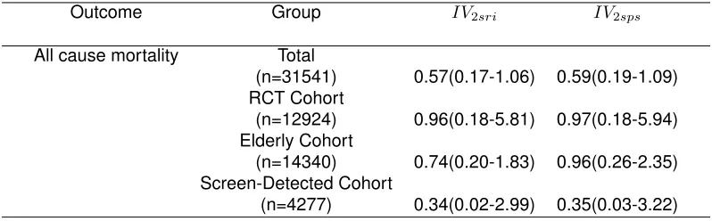
To assess the effectiveness of androgen deprivation with or without radiation therapy in reducing overall mortality (death from any cause), we performed two-stage IV Weibull regression analysis (2SPS and 2SRI) using a local area treatment rate instrument and controlling for the propensity score. The local area treatment rate instrument was defined as the proportion of patients who received definitive treatment (surgery or radiation therapy) among all patients with prostate can-cer in the hospital referral region (HRR) and we categorized this instrument into a binary variable according to its median. This IV measures the ‘aggressiveness’ of local area treatment and cap-tures regionally distinct structural care variation not fully explained by patient characteristics. The IV was strongly associated with treatment assignment and balanced important prognostic factors (Bekelman et al., 2015). The propensity score model included potential confounding variables in-cluding age, race, ethnicity, clinical T stage, N stage, and World Health Organization tumor grade, 17 categories of co-morbid disease, urban residence, and census track median income.

the hazard function is a decreasing one (α <1), the 2SPS method produces more stable and less biased estimates than the 2SRI method. In this case, 2SPS may be a more appropriate approach to use. In the RCT Cohort, the estimated HRs (HR=0.96) from both IV methods are much larger than the meta-analytic HR from the two randomized studies. Note that the confidence intervals are also much larger in both IV analyses than in the original RCTs. In the published RCTs, the authors concluded that there was a statistically significant treatment effect (combined therapy is better) whereas from our IV analysis, we can’t draw this conclusion. In the total study sample and separately in the RCT Cohort and the Screen-Detected Cohort, the two IV estimates are quite similar. However, for the Elderly Cohort, the estimate from the 2SPS method is different from the estimate from the 2SRI method.

2.7. Discussion

Many clinical and health services studies are using health care databases to compare the treat-ment effectiveness for drug and surgical therapies, but are prone to unmeasured confounding. Two stage IV methods have been gaining popularity among clinical researchers because these meth-ods provide a relatively simple approach to analyzing survival outcome studies in the presence of unmeasured confounding. However, current knowledge about potential bias in estimating the log causal hazard ratio is limited. As demonstrated in our prostate cancer study, the large treatment effects estimated from two stage IV methods could be attributable to potential bias. We have de-rived closed-form expressions for the asymptotic bias of the 2SRI and 2SPS approaches assuming the survival times follow a Weibull distribution with shape parameterαand scale parameterK. We have demonstrated that these analytic results are consistent with our simulation results.

of unmeasured confounding. In this case, we recommend exercising caution when interpreting results from two-stage IV survival models.

We have shown that even when all IV assumptions are met, both the 2SRI and the 2SPS methods could fail to consistently estimate the causal hazard ratio among compliers. Our analytic results for bias may help to guide researchers in deciding when the bias is likely to be reasonably small so that two stage IV methods may be reasonably applied. Furthermore, in a sensitivity analysis approach, one may estimate the shape parameter and the censoring proportion among patients assigned to treatment or control from the data. With the shape parameter and censoring proportions fixed based on our known data the level of the unmeasured confounding could be varied to examine how the estimates would change, as shown in Figures 1 and 2. Alternative methods include partial likelihood estimation (Cuzick et al., 2007).

2.8. Appendix

Appendix A: Mixture of Weibull Distributions

1) Prove the distribution function of observed survival timeT conditional on random assignmentR

can be expressed as the following equations:

F(T|R= 0) = 1−(e−( t θ1

AT

)α

ρA+e −( t

θ0

N T

)α

ρN +e −( t

θ0

C

)α

ρC) (A.1)

and,

F(T|R= 1) = 1−(e−( t θ1_C)

α ρC+e

−( t θ_{N T}0 )

α ρN +e

−( t θ_AT1 )

α

ρA) (A.2)

below:

R=1 if assigned to treatment;0 if assigned to control

Z=1 if receives treatment; 0 if receives control

ρr=P(R= 1)

ρA=P(AT)

ρC=P(C)

ρN = 1−ρA−ρC

T1₌

potential outcome for a patient under treatment

T0=potential outcome for a patient under control

T1

|AT _∼weibull(α, θ1

AT)

T1

|C_∼weibull(α, θ1

C)

T1|N T ∼weibull(α, θ1N T)

T0

|AT _∼weibull(α, θ0

AT)

T0

|C_∼weibull(α, θ0

C)

T0

|N T ∼weibull(α, θ0

N T)

Proof:

F(T(1)|Z= 1, R= 1) =P(T(1)≤t|Z= 1, R= 1)

= P(T

(1)

≤t, Z= 1, R= 1)

P(Z= 1, R= 1)

= P(T

(1)

≤t, AT, R= 1) +P(T(1)

≤t, C, R= 1) P(AT, R= 1) +P(C, R= 1)

= P(T

(1)

≤t, AT)P(R= 1) +P(T(1)

≤t, C)P(R= 1)

(P(AT) +P(C))P(R= 1) ∵R⊥(T

(1)

, T(0)),

R_⊥principal strata

= P(T

(1)

≤t|AT)P(AT) +P(T(1)

≤t|C)P(C)

P(AT) +P(C)

= (1₋e−( t θ1

AT

)α

) P(AT)

P(AT) +P(C)

+ (1₋e−( t θ1_C)

α

) P(C)

P(AT) +P(C)

F(T(0)

|Z= 0, R= 1) =P(T(0)

≤t_|Z= 0, R= 1)

= P(T

(0)

≤t, Z= 0, R= 1)

P(Z= 0, R= 1)

= P(T

(0)

≤t, N T, R= 1) P(N T)P(R= 1)

=P(T(0)

≤t_|N T) ∵R_⊥(T(1)_{, T}(0)_{), R}

⊥principal strata

= (1−e−( t θ0

N T

)α

F(T|R= 1)can be expressed as:

F(T|R= 1) =P(T ≤t, Z = 1|R= 1) +P(T ≤t, Z = 0|R= 1)

=P(T _≤t_|Z= 1, R= 1)P(Z = 1_|R= 1)

+P(T _≤t_|Z= 0, R= 0)P(Z= 0_|R= 1)

=P(T(1)≤t|Z= 1, R= 1)P(Z = 1|R= 1)

+P(T(0)

≤t_|Z = 0, R= 1)P(Z= 0_|R= 1)

= ((1₋e−( t θ1_AT)

α

) P(AT)

P(AT) +P(C)+ (1−e

−( t θ1_C)

α

) P(C)

P(AT) +P(C))(P(AT) +P(C))

+ (1₋e−( t θ0_{N T})

α

)(P(N T))

= 1−(e−( t θ_C1)

α ρC+e

−( t θ0_{N T})

α ρN +e

−( t θ1_AT)

α ρA)

F(T(1)

|Z= 1, R= 0) =P(T(1)

≤t_|Z= 1, R= 0)

= P(T

(1)

≤t, Z= 1, R= 0)

P(Z= 1, R= 0)

= P(T

(1)

≤t, AT, R= 0) P(AT, R= 0)

= P(T

(1)

≤t_|AT)P(AT)P(R= 0)

P(AT)P(R= 0)

=P(T(1)

≤t_|AT)

= 1−e−( t θ_AT1 )

F(T(0)|Z = 0, R= 0) =P(T(0)≤t|Z = 0, R= 0)

=P(T

(0)

≤t, Z = 0, R= 0)

P(Z = 0, R= 0)

=P(T

(0)

≤t, N T, R= 0) +P(T(0)

≤t, C, R= 0) P(N T, R= 0) +P(C, R= 0)

=P(T

(0)

≤t|N T)P(N T) +P(T(0)

≤t|C)P(C)

P(N T) +P(C)

= (1₋e−( t θ0

N T

)α

) P(N T)

P(N T) +P(C)

+ (1₋e−( t θ0_C)

α

) P(C)

P(N T) +P(C)

F(T_|R= 0)can be expressed as:

F(T|R= 0) =P(T ≤t, Z = 1|R= 0) +P(T ≤t, Z = 0|R= 0)

=P(T _≤t_|Z= 1, R= 0)P(Z = 1_|R= 0)

+P(T ≤t|Z = 0, R= 0)P(Z= 0|R= 0)

=P(T(1)

≤t_|Z= 1, R= 0)P(Z= 1_|R= 0)

+P(T(0)

≤t_|Z = 0, R= 0)P(Z= 0_|R= 0)

= ((1−e−( t θ1

AT

)α

)P(AT)

+ [(1₋e−( t θ0

N T

)α

) P(N T)

P(N T) +P(C)+ (1−e

−( t θ0

C

)α

) P(C)

P(N T) +P(C)](P(C) +P(N T))

= 1−(e−( t θ1

AT

)α

ρA+e −( t

θ0

N T

)α

ρN+e −( t

θ0

C

)α

ρC)

Appendix B: Proofs related with Derivation of Closed Form Solution

1) Assume survival time T _∼ W eibull(α, K) and censoring time L _∼ W eibull(α, λ). Let Y = min(T, L)andδ=I(T _≤L). Show that

Y _∼W eibull(α,( 1

λα +

1

Kα)−1/α)

and,

P(δ= 1) = 1

1 + Kα

λα

Proof:

P(Y ≥y) =P(min(T, L)≥y)

=P(T _≥y, L_≥y)

=

Z +∞

y

αt

α−1

Kαexp(−(

t K)

α_)dt

Z +∞

y

αl

α−1

λα exp(−(

l λ)

α_)dl

=exp(−(y K)

α

)exp(−(y λ)

α

)

=exp(−( y

( 1

λα+

1

Kα)−1/α

)α)

Thus,Y ∼W eibull(α,( 1

λα+

1

Kα)

−1/α₎

P(δ= 1) =P(0_≤T _≤L,0_≤L_{≤ ∞})

=

Z +∞ 0

αl

α−1

λα exp(−(

l λ)

α₎

Z l

0

αt

α−1

Kα exp(−(

t K)

α_)dtdl

=

Z +∞

y

αl

α−1

λα exp(−(

l λ)

α_)[1

−exp(−( l

K)

α_)]dl

= 1−

Z +∞

y

αl

α−1

λα exp(−(

l λ)

α

)exp(−( l K)

α

)dl

= 1₋ 1

1 + (λ/K)α

= 1

1 + (K

λ)α

2) Assume survival timeTis a mixture of three Weibull distributions with Densityf(t) =P3_i=1pif(ti).

T1 ∼ W eibull(α, K1), T2 ∼W eibull(α, K2), andT3 ∼W eibull(α, K3). The weights arep1, p2, p3

andP3i=1pi = 1. The censoring timeL ∼W eibull(α, λ). LetY = min(T, L)andδ =I(T ≤L).

Show that

P(δ= 1) =p1

1 1 + K1α

λα

+p2

1 1 + Kα2

λα

+p3

1 1 +Kα3

λα

Proof:

P(δ= 1) =P(δ= 1, G= 1) +P(δ= 1, G= 2) +P(δ= 1, G= 3)

=P(δ= 1_|G= 1)P(G= 1) +P(δ= 1_|G= 2)P(G= 2) +P(δ= 1_|G= 3)P(G= 3)

=p1

1 1 + K1α

λα

+p2

1 1 +Kα2

λα

+p3

1 1 +K3α

λα

3) Given X follows a Weibull distribution(α∗, K). Show that

E(Xα_{) = Γ(} α

α∗ + 1)K α

(B.3)

Proof:

E(Xα_{) =}

Z

Xα α∗

Kα∗X

α∗−1_e−(X

K)

α∗ dx

=

Z

yαα∗ 1

Kα∗e − y

Kα∗dy Lety=xα

∗

= 1

Kα∗ Z

y(αα∗+1)−1_e−

y

Kα∗dy

= 1

Kα∗(K

α∗₎(α

α∗+1)Γ(α

α∗ + 1)

Z ₁

(Kα∗

)(α

α∗+1)_Γ( α

α∗ + 1)

y(α

α∗+1)−1e− y

Kα∗dy

= Γ(α

α∗ + 1)K α

4) Given X follows a Weibull distribution(α∗_{, K). Show that}

E(log(X)) = −γ

Proof:

E(log(X)) =

Z ∞ 0

log(X) α

∗

Kα∗X

α∗−1

e−(XK) α∗

dx

=

Z ₁

α∗log(y)

1 Kα∗e

− y

Kα∗dy Lety=xα

∗

=

Z ₁

α∗(log(u) +α

∗_log(K))e−u_{du Lety=uK}α∗

= 1

α∗ Z

log(u)e−udu

| {z } −γ

+log(K)

Z

e−udu Lety=uKα∗

= −γ

α∗ +log(K)

5) Given X follows a Weibull distribution(α∗_{, K). Show that}

E(Xα_log(X)) 1

α∗Γ(

α

α∗ + 1)(K

α_)(ψ(α

α∗ + 1) +α

∗_log(K))

(B.5)

Proof:

E(Xα_{log(X)) =}

Z ∞ 0

Xα_log(X) α∗

Kα∗X

α∗−1_e−(X

K)

α∗ dx

=

Z

yαα∗ 1 α∗log(y)

1 Kα∗e

− y

Kα∗dy Lety=xα

∗

= 1

α∗

1 Kα∗Γ(

α

α∗ + 1)(K

α∗₎α

α∗+1

Z

log(y) 1

Γ(α

α∗+ 1)(Kα ∗

)αα∗+1 y(α

α∗+1)−1e− y

Kα∗dy

| {z }

E(log(y))

y_∼gamma( α α∗ + 1, K

α∗₎

= 1

α∗

1 Kα∗Γ(

α

α∗ + 1)(K

α∗

)αα∗+1_(ψ(α

α∗ + 1) +α

∗_{log(K)) ψ()is digamma function}

= 1

α∗Γ(

α

α∗ + 1)(K

α_)(ψ(α

α∗ + 1) +α

∗_log(K))

6) Let Ti denote the survival time andCi denote the censoring time for subjecti. Ti andCi are

independent. Ti ∼ weibull(α, K), andCi ∼ weibull(α, λ). LetYi =min(Ti, Ci)denote observed

follow-up time andδi be the indicator variableδi = (Ti≤Ci). Show that: