A Computer Aided Diagnosis System for Lung Cancer based on Statistical and Machine Learning Techniques

A Computer Aided Diagnosis System for Lung

Cancer based on Statistical and Machine

Learning Techniques

Hamada R. H. Al-Absi1_{, Brahim Belhaouari Samir}2*_{, Suziah Sulaiman}1

1_{Department of Computer & Information Sciences, Faculty of Science and Information Technology} Universiti Teknologi PETRONAS, 31750 Tronoh, Perak, Malaysia

2_{College of Science, ALFAISAL University, P.O.Box 50927, Riyadh 11533, Kingdom of Saudi Arabia} Email: [email protected], [email protected], [email protected]

Abstract— lung Cancer is believed to be among the primary factors for death across the world. Within this paper, statistical and machine learning techniques are employed to build a computer aided diagnosis system for the purpose of classifying lung cancer. The system includes preprocessing phase, feature extraction phase, feature selection phase and classification phase. For feature extraction, wavelet transform is used and for feature selection, two-step statistical techniques are applied. Clustering-K-nearest-neighbor classifier is employed for classification. The Japanese Society of Radiological Technology’s standard dataset of lung cancer has been utilized to evaluate the system. The dataset has 154 nodule regions (abnormal) - where 100 are malignant and 54 are benign - and 92 non-nodule regions (normal). An Accuracy of 99.15% and 98.70 % for classification have been achieved for normal versus abnormal and benign versus malignant respectively, this substantiate the capabilities of the approach presented in this paper.

Indexed Terms — Computer Aided Diagnosis, Lung Cancer, Statistical Feature Selection, Cluster k-Nearest Neighbor term

I. INTRODUCTION

Cancer is a disease that is referred to as the number one cause of death worldwide. According to the World Health Organization (WHO) [1], cancer was the reason for 7.4 million deaths (13% of all deaths) occured in 2008. More than 70% of all cancer deaths occur in middle income nations. It is projected that deaths caused by cancer will be growing to reach 13.1 million by the year 2030 [1].

Lung cancer is a form of cancer that has become a significant cause of death globally [2]. According to GLOBOCAN Project – which is carried out by the International Agency for Research in Cancer (An agency of the WHO) – lung cancer has accounted for 12.7 % of the total cancer incidents and 18.2 % of the total mortality caused by cancer, both rates are more than any other form of cancer. Figure 1 shows a summary for the cancer

incident and mortality rates in both sexes worldwide as it was published by GLOBOCAN project [3].

Figure 1. Cancer incidence and mortality rates [3]

Given that the cause of cancer remains unknown, early detection and treatment of cancer is the most promising ways to reduce the number of deaths. In order to diagnose cancer, medical imaging modalities such as Mammography, Computed Tomography and Magnetic Resonance Imaging, etc. have been developed to produce images of body organs that help to identify abnormalities. Radiologists and physicians depend on these images to diagnose diseases; yet, radiologists are incapable of indentifying subtle regions. For that, Computer Aided Diagnosis (CAD) systems have been designed to assist radiologist to recognize subtle regions and discover malginant (cancerous) cells [4].

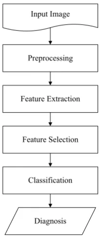
CAD methods are generally designed to guide radiologists in diagnosing pulmonary nodules which necessarily suggest the presence of lung cancer. CAD systems typically incorporate four stages; preprocessing, feature extraction, feature selection and classification. Figure 2 shows a block diagram of the primary computer aided diagnosis system's elements.

Input Image

Preprocessing

Feature Extraction

Feature Selection

Classification

Diagnosis

Figure 2. General block diagram for CAD system

As this is a significant area of research, many CAD systems have been developed for lung cancer and for many other types of cancer. However, High false positives and detecting subtle regions are still among the issues that researchers are working to tackle. CAD systems with high false positive decrease the efficiency of the diagnosis [5], therefore, the number of false negatives should be decreased.

II. RELATED WORK

Large numbers of Computer Aided Diagnosis systems have previously been designed in the area of cancer diagnosis. For lung cancer, Hardie et al. [6] designed a CAD technique for lung nodule detection in chest radiography. The system had been evaluated with a data set which contains 167 chest radiography containing 181 lung nodules; the technique employed adaptive distance-based threshold algorithm for nodule segmentation. Thereafter, features were calculated from each nodule using geometric features, intensity features and gradient features. Finally, a Fisher linear discriminant classifier was adopted to classify the calculated features. The system's accuracy was 78.1%. Chen et al [7] presented a computer aided diagnosis for lung nodules on CT images. The system utilized Neural Network ensemble-based classifier for the classification of benign and malignant nodules. The system attained an Az value of 0.915.

Lee et al. [8] presented a lung nodule detection employing an ensemble classifier assisted by clustering.

Lung images of 32 individuals which enclosed 5721 images have been used to examine the technique. The system attained sensitivity of 98.33% and specificity of 97.11%. Tan et al [9] developed a system for the detection and classification of lung nodules. Vessel enhancement filters and a computed divergence feature to locate the centers of the nodule clusters. After that, the detected nodules are subjected to a classification stage where invariant features are classified through a feature selective classifier based on Genetic Algorithm and Artificial Neural Network. The classifier is compared with fixed-topology neural network and support vector machine classifiers. Results show that the fixed-topology neural network performs better than the other classifiers where a detection rate of 87.5% is achieved. A system has been presented by Dehmeshki et al. [10] in order to detect lung nodules making use of shape-based genetic algorithm template matching (GATM). In this system, a preprocessing enhancement step had been conducted making use of spherical-oriented convolution-based filtering scheme, and a 3D geometric shape feature has been utilized to determine the fitness function. The system had been examined with a dataset of 70 CT images comprising 178 nodules. The system attained an accuracy rate of 90%. Another system has been proposed by Pereira et al [11] which presented a technique for lung nodule classification with multiclassifiers. The technique begin by filtering images utilizing a multi-scale filter bank which comprise of 36 filters at various scales and orientation, isotropic filters, gaussian and laplacian of gaussian. A multiple classifiers based on different multiple-layer perceptron (MLP) were utilized to classify the images. The system was examined with JSRT dataset, with 19 classifier combination; the Borda count combination attained 97% sensitivity with 43% error. A computerized method for lung cancer detection has also been designed by Sousa et al. [12]. The system has six stages, namely, thorax extraction, lung extraction, lung reconstruction, structure's extraction, tubular structures elimination, and false-positive reduction. Every single stage carries out a particular activity which leads to detecting lung nodules. The sensitivity attained was 84.84%, and specificity attained was 96.15%.

III MATERIALS AND METHODS A. Dataset

In this paper, the Japanese Society of Radiological Technology (JSRT) standard dataset of chest radiographs [14-15] is utilized to evaluate the method. The dataset includes 247 chest radiographs. Table I shows the distribution of the dataset images.

TABLEI

JSRTDATASETIMAGESDISTRIBUTION

Benign Malignant Total

Abnormal (Nodule) 54 100 154

Normal (Non-nodule) - - 93

Total Images 247

Regions of 128x128 were extracted from the original 2048x2048 images. For the abnormal (nodule) regions, the regions have been extracted based on the provided coordinates of all the 154 nodules images. Figure 3 shows an example of one chest radiography.

Figure 3. Example image of the JSRT (JPCLN001.IMG) [14]

B. Methods

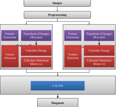
This section presents a computer aided system for lung cancer diagnosis. The section is divided into parts; each one explains a processes. Figure 4 shows the components of the proposed system.

Preprocessing

Training Phase _{Testing Phase}

Transform of Images (Wavelet) Calculate Energy Calculate Statistical

Metric (s)

Classification Phase

C-K-NN

Diagnosis

Feature Extraction

Feature Selection

Transform of Images (Wavelet) Calculate Energy Calculate Statistical

Metric (s) Feature

Extraction

Feature Selection

Images

Figure 4. Proposed CAD system for lung cancer classification

 Preprocessing

Two preprocessing techniques are employed in this CAD system. The first technique is histogram equalization to enhance the contrast of the image so the intensity levels (which will be in the range [0 1]) would generate a flat histogram.

Let 𝑝𝑟

(

𝑟𝑗

)

, 𝑗= 1,2,…,𝐿 _{represent a particular image’s} histogram intensity level. The histogram equalization transformation shall be:

𝑠_𝑘 = 𝑇

(

𝑟_𝑘

)

= 𝑘

∑

𝑗= 1

𝑝_𝑟

(

𝑟_𝑗

)

= 𝑘

∑

𝑗= 1

𝑛_𝑗

𝑛 (1)

for k = 1,2,…,L. where 𝑟𝑘 _{is the intensity value of the} input image and 𝑠𝑘 _{is the intensity value of the output} image [16]. Figure 5 demonstrates a lung sub-image before and after implementing histogram equalization.

a b

c b

Figure 5. Histogram equalization effect on the image. (a) Original Image (b) Original Image’s Histogram. (C) Image after applying

Histogram Equalization. (d) Equalized image histogram

The second technique is image filtering. Laplacian filter is utilized to spotlight the rapid intensity change in regions within an image.

 Feature Extraction using Wavelet Transform

The transform of a signal is regarded as an alternative way of presenting the signal. And it also saves the important information contained in the signal. Wavelets employ various sets of fundamental functions to allow for the decomposition of continuous and discrete signals. Wavelet Transform provides a time-frequency description of the signal.

utilized in the transformation through translation (shifting) and scaling.

1 * t-τ

X_WT(τ,s)= x(t).Ψ dt s s 













(2)

The Wavelet Transform is a multiresolution method that has been widely employed in feature extraction because of the excellent performance in contrast to other feature extraction techniques. An in-depth description of wavelets and its concept is available at mallat [17].  Feature Selection

It is essential to lower the number of the coefficients generated by the wavelet [18]. This can be done by determining those coefficients which contains relevant information only.

The selected features are computed in two stages, which are calculating a statistical energy as well as a statistical metric. In both stages, only features less than a specific threshold are selected. Details of the two stages are as follows:

Statistical Energy: This can be calculated as follows:

𝐸𝑛𝑒𝑟𝑔𝑦_𝑚𝑒𝑡𝑟𝑖𝑐(𝑘) =

∑

𝑖

∑

𝑗

|

𝑛𝑖_𝑗(𝑘)

|

∑

𝑖

𝑛_𝑖(𝑘) (3)

𝑤ℎ𝑒𝑟𝑒 𝑛_𝑗𝑖(𝑘) 𝑖𝑠 𝑓𝑒𝑎𝑡𝑢𝑟𝑒 𝑘 𝑜𝑓 𝑖𝑚𝑎𝑔𝑒 𝑗 𝑖𝑛 𝑐𝑙𝑎𝑠𝑠 𝑖 .

After calculating the statistical energy, all energy values less than a certain threshold are removed.

Statistical Metric: This can be calculated as follows: Assume m1, m2 and m3 are the mean of class1, class2, and

class3, respectively and 𝑚𝑇 _{is the mean of all classes.}

𝐿𝑒𝑡 𝑚_𝑇(𝑘) = 𝑛

∑

𝑖= 1

𝑚_𝑖(𝑘)

𝑛 _{Where n = number of classes, so}

𝑣𝑎𝑟_𝑚𝑜𝑑(𝑘)=_𝑛1

∑

(

𝑚_𝑖(𝑘) ‒ 𝑚_𝑇(𝑘)

)

(4)

however,

∑

(𝑚𝑖(𝑘) ‒ 𝑚𝑇(𝑘))2 _{is not adequate to} measure the classification contribution of the coefficients because it may provide similar values in the two cases. For that reason, there exists a need to present a different metric to measure the coefficients’ contribution. The metric is as follows:

𝑉𝑎𝑟_𝑚𝑜𝑑(𝑘)= min

𝑖 ≠ 𝑗

|

𝑚_𝑖(𝑘)‒ 𝑚_𝑗(𝑘) 𝑆2_𝑖(𝑘) 𝑛_𝑖(𝑘)+

𝑆2_𝑗(𝑘) 𝑛_𝑗(𝑘)

|

(5)

where𝑆𝑖 _{is the statistical metric of class} 𝑖_, 𝑚𝑖 _{is the mean} of class 𝑖_{, and} 𝑛𝑖 _{is the number of classes.} 𝑆𝑖 _{can be} calculated as follows:

𝑆2_𝑖= 𝑛_𝑖

∑

𝑗= 1

(

𝑥𝑖_𝑗(𝑘)‒ 𝑚_𝑖(𝑘)

)

2

𝑛_𝑖‒1

(6)

where i=1, 2, 3, …, ni, and 𝑛𝑖 is the number of the

features in class 𝑖_.

 classification

A classifier which is a combination of K-means modified algorithm and K-Near Neighbor (K-NN) is used within this study. This classifier was introduced by Samir Brahim [13]. The classifier is called Cluster K-Nearest Neighbor (C-K-NN). The algorithm is explained further below:

Every single class,𝐶𝑖 s should become a cluster to various subclasses, 𝐶𝑖,𝑗, with 1≤ 𝑗 ≤1, and each subclass will be represented by its mean, μ𝑖,𝑗. Hence, the cluster analysis determines a set of groups, which will decrease the within-group variation and increase the between-group variation. K-means cluster algorithm is applied for every class for clustering purposes then both the number of subclasses for every class and the initial k-vectors to initialize the K-means cluster algorithm are defined to find the ideal number of the subclasses. The number of subclasses is iterated beginning with 1 and the irritation process should stop by the following two conditions:

o All the representatives, μ𝑖,𝑗, should be close with respect to the metric 𝑑 _{of their classes,} 𝐶𝑖 _{, ( i.e., if we} classify all the representatives, μ𝑖,𝑗 _{, we have found} 100% accuracy). If there are some misclassifications ofμ𝑖,𝑗_{, we have to decrease the parameter} α _by multiplying it with another factor,α'_{, which is less}

than 1.

o The statistical metric of each class 𝐶𝑖, 𝑣𝑎𝑟𝑖, does not decrease significantly in comparison to the previous iteration.

We may use

△ 𝑉𝑎𝑟

𝑉𝑎𝑟 ≤ α_{as a criterion to quantify if}

there is a decrease or it still approximately remains constant. In certain cases, it is better to stop the iteration

if the condition

△ 𝑉𝑎𝑟

𝑉𝑎𝑟 ≤ α _{has been checked twice or}

more (i.e., after which the statistical metric will be smoothened).

For initialization of the K-means cluster algorithm in general, we choose k-vectors, which belong to our classes' data. This will therefore make the algorithm unstable in the sense of the final variance:

𝑣𝑎𝑟 𝐶_𝑖= 𝑚_𝑖

∑

𝑗= 1

𝑣𝑎𝑟 𝐶_𝑖,𝑗

which depends on the initial vectors.

From here, the question "How to choose the initial vectors in order to find a minimal variance?" arises. To answer this, in this paper, we have developed two algorithms: the Hierarchical Near-to-Near and Hierarchical Near-to-Mean algorithms, which might require some modification for different applications.

Hierarchical Near-to-Near Algorithm

This algorithm consists of calculating the distance

𝑑(𝑥_𝑖,𝑛 , 𝑥_𝑖,𝑚) _{for all} 𝑥_𝑖,.∈ 𝐶_{𝑖 and starting to cluster our}

classes to 𝑁𝑖‒1 _{subclasses where} 𝑐𝑎𝑟𝑑

(

𝐶𝑖

)

= 𝑁𝑖_{. We} put the two closest data in the same subclasses

where 𝑛 ≠ 𝑚𝑚𝑖𝑛 𝑑

(

𝑥𝑖,𝑛 , 𝑥𝑖,𝑚

)

= 𝑑

(

𝑥𝑖,𝑛𝑜 , 𝑥𝑖,𝑚𝑜

)

,

and we put each of the other data in separate subclasses,

𝐶_𝑖,𝑗=

{

𝑥_𝑖,𝑗

}

, ∀𝑗 ∈{1,…., 𝑁}‒

{

𝑛_𝑜,𝑚_𝑜

}

.

In the next step, the following index 𝑛1 _and 𝑚1_are considered for which

𝑚𝑖𝑛 𝑛 ≠ 𝑚 (𝑛,𝑚)≠ (𝑛𝑜,𝑚𝑜)

𝑑

(

𝑥_𝑖,𝑛 , 𝑥_𝑖,𝑚

)

= 𝑑

(

𝑥_𝑖,𝑛1 , 𝑥_𝑖,𝑚1

)

.

If 𝑥𝑖,𝑛1_and 𝑥𝑖,𝑚1 _{belong to the same subclass,}𝐶𝑖,𝑟_{, we} shall split this subclass into two other subclasses:

𝐶_{𝑖,𝑟+ 1}= 𝐶_𝑖,𝑟‒

{

𝑥_𝑖,𝑛1 , 𝑥_𝑖,𝑚1

}

(7)

𝐶_𝑖,𝑟=

{

𝑥_𝑖,𝑛1 , 𝑥_𝑖,𝑚1

}

(8)

In the case where 𝑥𝑖,𝑛1_and 𝑥𝑖,𝑚1_{belong to two different} subclasses, 𝐶𝑖,𝑟1 _and 𝐶𝑖,𝑟2_{, respectively, we shall put} 𝑥𝑖,𝑛1 in the subclass, 𝐶𝑖,𝑟2_{, if} 𝑐𝑎𝑟𝑑( 𝐶𝑖,𝑟2) > 𝑐𝑎𝑟𝑑( 𝐶𝑖,𝑟1) _and we may put𝑥𝑖,𝑚1_{in the subclass ,} 𝐶𝑖,𝑟1 _{, if}

𝑐𝑎𝑟𝑑( 𝐶_𝑖,𝑟2)≤ 𝑐𝑎𝑟𝑑( 𝐶_𝑖,𝑟1)_{. Indeed, to get the cardinality} of the set we may use the distance between the vectors to the set as 𝑑(𝑣𝑒𝑐𝑡𝑜𝑟,𝑚𝑒𝑎𝑛 𝑜𝑓 𝑠𝑒𝑎𝑡)_{. When we obtain} 𝑘

subclasses, we stop the iteration, and our initial k-vectors will be the mean of each subclass.

Hierarchical Near-to-Mean Algorithm

This algorithm is almost the same as the Hierarchical Near-to-Near algorithm, except we will deal with the mean of subclass 𝐶𝑖,𝑟 _{in the processing. We start by} splitting our class 𝐶𝑖 _{into two subclasses:}

𝐶_𝑖,1=

{

𝑥_{𝑖,𝑛𝑜}, 𝑥_{𝑖,𝑚𝑜}

}

(9)

and

𝐶_𝑖,2=

{

𝑥_𝑖,𝑗

│

𝑗 ∉

{

𝑛_𝑜, 𝑚_𝑜

}}

, ₍₁₀₎

where 𝑑

(

𝑥𝑖,𝑛𝑜 , 𝑥𝑖,𝑚𝑜

)

=_{𝑛 ≠ 𝑚}𝑚𝑖𝑛 𝑑(𝑥𝑖,𝑛 , 𝑥𝑖,𝑚)

We then updated our classes, 𝐶𝑖 _{, by replacing} 𝑥𝑖,𝑛𝑜 _and

𝑥_{𝑖,𝑚𝑜 with their average,}

𝐶1_𝑖=

{

…,𝑥_{𝑖,𝑛𝑜 ‒1},𝑆₀,𝑥_{𝑖,𝑛𝑜+ 1},…,𝑥_{𝑖,𝑚0 ‒1},𝑆₀,𝑥_{𝑖,𝑚𝑜+ 1},…

}

Where 𝑠𝑜=(𝑥𝑖,𝑛𝑜+ 𝑥𝑖,𝑚𝑜)/2 Next, we consider 𝑥𝑖,𝑛1 _and 𝑥𝑖,𝑚1 _as:

𝑑

(

𝑥_𝑖,𝑛1 , 𝑥_𝑖,𝑚1

)

=𝑚𝑖𝑛

{

𝑑(𝑥_𝑖,𝑛 , 𝑥_𝑖,𝑚)

│

𝑑(𝑥_𝑖,𝑛 , 𝑥_𝑖,𝑚)≠0

}

We then replace 𝐶1𝑖 _{and all the data in} 𝐶1𝑖 _{that are} equal to 𝑥𝑖,𝑛1 _or 𝑥𝑖,𝑚1 _by 𝑆1_{, which is the mean of the} union of the two subclasses where 𝑥𝑖,𝑛1 _and 𝑥𝑖,𝑚1 _belong to:

𝑆₁=𝐶𝑛1𝑥_𝐶𝑖,𝑛1+ 𝐶𝑚1𝑥𝑖,𝑚1

𝑛1+ 𝐶𝑚1 (11)

where 𝐶𝑛1 _{is the number of the repetitions of} 𝑥𝑖,𝑛1 _inside of 𝐶1𝑖_{, and} 𝐶𝑚1 _{is the number of the repetitions of} 𝑥𝑖,𝑚1 inside of 𝐶1𝑖_{. Our algorithm stops once the number of} distinct vectors inside of 𝐶𝑟𝑖 _{is equal to k. Our}

classification algorithm does not need to keep all the data, only the average of each subclass. This is the outstanding feature of this new clustering. To classify a new data or vector 𝑥_{, we use k-NN algorithm, i.e., we assign} 𝑥 _{to the}

class 𝐶̂𝑖 _{for which:}

̂𝑖=𝑎𝑟𝑔_𝑖𝑚𝑖𝑛_𝑖,𝑗 𝑑

(

𝑥,μ_𝑖,𝑗

)

(12)

Where 𝑎𝑟𝑔𝑖 𝑑

(

𝑥,μ𝑖0,𝑗0

)

=𝑖0_.

IV RESULTS AND DISCUSSION

In this paper, two experiments have been carried out. The first experiment is to classify normal from abnormal images and the second experiment to classify benign from malignant images. The following sub-sections report the results obtained for both experiments.

A. Classification Performance

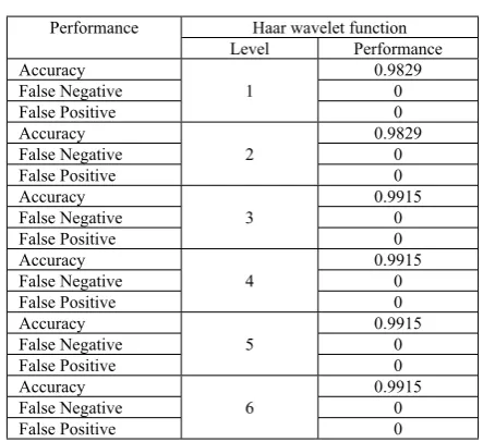
In this section, the performance of the methods on classifying normal from abnormal images as well as benign from malignant images is demonstrated. The accuracy, false negatives and false positives are shown in table II when Haar Wavelet was utilized for the Normal vs. Abnormal experiment. The performance reached 99.15 % accuracy rate with zero false positives and zero false negatives with Haar Wavelet levels 3, 4, 5 and 6.

TABLEII

PERFORMANCE OF THE METHODS ON NORMAL VS.ABNORMAL

CLASSIFICATION

Haar wavelet function Performance

Level Performance

Accuracy 0.9829

False Negative 0

False Positive

1

0

Accuracy 0.9829

False Negative 0

False Positive

2

0

Accuracy 0.9915

False Negative 0

False Positive

3

0

Accuracy 0.9915

False Negative 0

False Positive

4

0

Accuracy 0.9915

False Negative 0

False Positive

5

0

Accuracy 0.9915

False Negative 0

False Positive

6

0

Furthermore, when the Haar Wavelet function was applied to the benign against malignant experiment, the performance reached 98.70 % accuracy with zero false negatives and false positives at the function levels 1,2,4 and 6. Table III reports the results obtained at different function level.

TABLEIII

PERFORMANCE OF THE METHODS ON BENIGN VS.MALIGNANT

CLASSIFICATION

Haar wavelet function Performance

Level Performance

False Negative 0

False Positive 0

Accuracy 0.9870

False Negative 0

False Positive

2

0

Accuracy 0.9870

False Negative 0.0200

False Positive

3

0

Accuracy 0.9870

False Negative 0

False Positive

4

0

Accuracy 0.9870

False Negative 0.0200

False Positive

5

0

Accuracy 0.9870

False Negative 0

False Positive

6

0

B. Usefulness of Feature Selection

Feature selection has an influence on the performance of our computer aided diagnosis systems. It works to eliminate repetitive and needless information which was extracted during the feature extraction stage. Table IV shows how our two-step feature selection methods have reduced the number of coefficients extracted by the haar wavelet.

TABLEIV

THE AFFECT OF FEATURE SELECTION ON REDUCING THE NUMBER OF COEFFICIENTS

Experiment Normal

Vs. Abnormal

Benign Vs. Malignant Haar Wavelet function Level 3 2

Initial coefficients 16384 16384 After Energy calculation 6562 11470 After Statistical Metric calculation 291 291

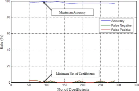
To show the effectiveness of the feature selection step, figure 6 shows an illustration when the haar wavelet with level 3 was used on the Normal Vs. Abnormal experiment. In this figure, the influence of the number of coefficients is noticed where the highest accuracy with minimal false negatives and false positive occurs at the ideal number of features (coefficients).

Figure 6. The affect of the No. of Coefficients to the performance

C. Cross Validation

Cross validation is a statistical approach to assess learning algorithms. It operates by splitting the data into two parts, one is used to train and the other to test. Cross validation is available in many strategies; in this paper, the k-fold strategy is utilized to validate the system. A 10-fold cross validation was performed on the Haar Wavelet with the highest performance for each experiment. Table V reports the results for the cross validation.

The averaged accuracy obtained after the cross validation was 98.75 % for the Normal Vs. Abnormal experiment; while it was 98.70 for the Benign Vs. Malignant experiment. This shows the effectiveness of our computer aided diagnosis system and its ability to diagnose lung nodules.

TABLEV

10-FOLD CROSS VALIDATION RESULTS ON BOTH EXPERIMENTS

Experiments

k-folds _{Normal Vs. Abnormal Benign Vs. Malignant}

Fold 1 100 98.70

Fold 2 95.83 97.40

Fold 3 95.83 100

Fold 4 100 98.70

Fold 5 100 98.70

Fold 6 100 98.70

Fold 7 100 98.70

Fold 8 100 98.70

Fold 9 100 98.70

Fold 10 95.83 98.70

Average 98.75 98.70

V CONCLUSION AND FUTURE WORK

The paper introduced a computer aided diagnosis system for lung nodules based on cluster k nearest neighbor algorithm and statistical feature selection methods. The results shown in the previous section proves the capabilities of the CAD system in lung cancer classification (Normal Vs. Abnormal and Benign Vs. Malignant). A 99.15 % and 98.70 % accuracy rates have been achieved for the normal vs. abnormal and benign vs. malignant experiments respectively with zero false positives and false negatives. The methods were verified with Cross Validation and the results obtained prove the advantage of the proposed system. Further experiments will be performed to examine the methods in other datasets with different modalities (i.e. CT scan) as well as other forms of cancer.

ACKNOWLEDGMENT

PETRONAS, Malaysia, for supporting this work with the Graduation Assistantship Scheme.

REFERENCES

[1] World Health Organization (WHO), “Cancer facts sheet, 2010”

http://www.who.int/mediacentre/factsheets/fs297/en/ (Accessed October 2013)

[2] Qiang Li, Recent progress in computer-aided diagnosis of lung nodules on thin-section CT. Computerized Medical Imaging and Graphics 31 (2007); pp. 248–257.

[3] GLOBOCAN, Cancer Fact Sheet 2008, http://globocan.iarc.fr/factsheet.asp

(Accessed October 2013).

[4] J. Tang, R. Ranjayyan, I. El Naqa, Y. Yang, Computer aided detection and diagnosis of breast cancer with mammogram: recent advances. IEEE Transaction Information Technology in Biomedicine, 13 (2), 2009, pp. 236-251.

[5] S. A. Taylor, et al., "Influence of Computer-Aided Detection False-Positives on Reader Performance and Diagnostic Confidence for CT Colonography," American Journal of Roentgenology, vol. 192, pp. 1682-1689, June 1, 2009 2009.

[6] R C. Hardie, Steven K. Rogers, Terry Wilson, Adam Rogers; Performance analysis of a new computer aided detection system for identifying lung nodules on chest radiographs. Medical Image Analysis 12 (2008); pp. 240– 258.

[7] H. Chen, Y. Xu, Y. Ma, and B. Ma, “Neural network ensemblebased computer-aided diagnosis for differentiation of lung nodules on CT images: clinical evaluation,” Academic Radiology,vol. 17, no. 5, pp. 595– 602, 2010.

[8] S.L.A. Lee, A.Z. Kouzani, E.J. Hu, Random forest based lung nodule classification aided by clustering. Computerized Medical Imaging and Graphics 34 (2010); pp. 535–542

[9] M. Tan, R. Deklerck, B. Jansen Nad, M. Bister, and J. Cornelis, “A novel computer-aided lung nodule detection system for CT images,” Medical Physics, vol. 38, no. 10, pp. 5630–5645, 2011.

[10] J. Dehmeshki, Xujiong Ye, XinYu Lin, Manlio Valdivieso, Hamdan Amin; Automated detection of lung nodules in CT images using shape-based genetic algorithm. Computerized Medical Imaging and Graphics 31 (2007); pp.408–417 [11] C. Pereira, et al., "A Multiclassifier Approach for Lung

Nodule Classification," in Image Analysis and Recognition. vol. 4142, A. Campilho and M. Kamel, Eds., ed: Springer Berlin Heidelberg, 2006, pp. 612-623. [12] J. R. F. Sousa, Aristófanes Corrˇea Silva, Anselmo

Cardoso de Paiva, Rodolfo Acatauassú Nunes,

Methodology for automatic detection of lung nodules in computerized tomography images. Computer Methods and Programs in Biomedicine 98 (2010); pp. 1–14.

[13] Brahim Belhaouari, samir (2009) Fast and Accuracy Control Chart Pattern Recognition using a New cluster-k-Nearest Neighbor. Journals of Word Academy of Science, Engineering and Technology.

[14] Shiraishi J, Katsuragawa S, Ikezoe J, Matsumoto T, Kobayashi T, Komatsu K, Matsui M, Fujita H, Kodera Y, and Doi K.: Development of a digital image database for chest radiographs with and without a lung nodule: Receiver operating characteristic analysis of radiologists' detection of pulmonary nodules. AJR 174; 71-74, 2000

[15] Japanese Society of Radiological Technology Lung Dataset.

http://www.jsrt.or.jp/web_data/english01.html?category=3 (Accessed: October 2011)

[16] R. C. Gonzalez, et al., Digital Image Processing Using

MATLAB, 1st ed.

[17] S. G. Mallat, "A theory for multiresolution signal decomposition: the wavelet representation," Pattern Analysis and Machine Intelligence, IEEE Transactions on, vol. 11, pp. 674-693, 1989.

[18] H. R. H. Al-Absi, Brahim B. Samir, Khaled Bashir Shaban, and Suziah Bt. Sulaiman, “Computer Aided Diagnosis System based on Machine Learning Techniques for Lung Cancer,” International Conference on Computer and Information Sciences (ICCIS2012), Kuala Lumpur, Malaysia, June 12-14, 2012.

Hamada R. H. Al-Absi has obtained his Bachelor of Technology in Information & Communication Technology and Master of Science in Information Technology in 2009 and 2010 respectively from Univeristi Teknology PETRONAS, Perak, Malaysia. Currently he is pursuing his PhD at the department of Computer and Information Sciences at Universiti Teknologi PETRONAS, Malaysia. His research interests are in pattern recognition and machine learning.

Brahim Belhaouari Samir received his Master degree from INP/EENSET Toulouse, France 2000 and Ph.D. in Stochastic Processes from EPFL, Lausanne Switzerland in 2006. After completing the Ph.D. degree, he held a Postdoctoral at Ecole Polytechnique Federale De Lausanne, Lausanne, Switzerland. Now, he is an assistant professor at the College of Science and General Studies, Alfaisal University, Kingdom of Saudi Arabia. His main research interests are in data analysis, statistical signal processing, and pattern recognition.