A Method for Diagnosing the Condition of Energy Elements, Control And Management Of Energy Efficiency Of Energetic Consumption Systems

International Journal of Research in Engineering and Science (IJRES)

ISSN (Online): 2320-9364, ISSN (Print): 2320-9356

www.ijres.org Volume 2 Issue 4 ǁ April. 2014 ǁ PP.38-43

A Method for Diagnosing the Condition of Energy Elements,

Control And Management Of Energy Efficiency Of Energetic

Consumption Systems

V.Karpov

, T. Kabanen

, J. Resev

1_{Saint-Petersburg state Agrarian University, Pushkin-1,Box No 1, 196600, St.-Petersburg, Russia.}

2_{Tallinn University of Technology Tartu Colleg , Puiestee 78,51008 Tartu, Estonia.}

3

Tallinn University of Technology Tartu Colleg , Puiestee 78,51008 Tartu, Estonia..

ABSTRACT :To implement the method of diagnosing the elements of energetic consumption systems (ECS) , all production processes are broken into three categories: basic energy technological processes of obtaining products (ETP1), auxiliary energy technological processes (ETP2) and energy technological processes which ensure living conditions (ETP3).

Technical diagnostics determines the technical condition of an element which is characterized at a specific time and in certain environmental conditions by the values of parameters defined in the technical documents of the elements. As a result of technical diagnostics, one of two working conditions of elements is determined: usable or unusable. During the energy diagnostics of ECS, the element’s condition and ETP are determined by calculating their relative energy consumption and energy efficiency (for example, specific energy consumption per unit of production).

The developed method of diagnostics allows comparing the losses in elements depending on the load which varies with time and determining the increase in energy losses in the element. It also allows determining the proportion of runtime under equal loads, and the load creating the maximum energy loss, i.e., the most energy-consuming mode in which the deterioration of the element’s condition has the greatest effect on energy losses in this ETP .Losses are minimized by changing or limiting the operation of or restoring the condition of the element.

Keywords: energy efficiency, economic effectiveness

I.

INTRODUCTION

To implement the method of diagnosing the elements of energetic consumption systems (ECS) , all production processes are broken into three categories: basic energy technological processes of obtaining products (ETP1), auxiliary energy technological processes (ETP2) and energy technological processes which ensure living conditions (ETP3).

Technical diagnostics determines the technical condition of an element which is characterized at a specific time and in certain environmental conditions by the values of parameters defined in the technical documents of the elements. As a result of technical diagnostics, one of two working conditions of elements is determined: usable or unusable. During the energy diagnostics of ECS, the element’s condition and ETP are determined by calculating their relative energy consumption and energy efficiency (for example, specific energy consumption per unit of production).

II.

MATERIALS AND METHODS

The method of diagnosing the condition of energy elements, control and management of energy efficiency of consumer energy system, which is based on finite ratio method (FRM) [1], requires the simultaneous and continuous registration of energy values on input and output of elements and ETP [2]. Based on the registered parameters for a representative period of time, the specific energy consumption per unit of production P is determined.

This is achieved by determining the value of energy consumption at the beginning of each line containing ETP:

- Qpr is energy consumed for producing production P in line containing ETP1: P

spec pr Q el Q pr

Q  ₁  (1)

Where: Qel1 is the power intensity of the line feeding ETP1; - _Qspec_pr is the specific power intensity of a product P;

2 2

2 2

R spec R Q el Q R

Q    (2)

Where: Qel2 is the power intensity of the line feeding ETP2; spec

R

Q ₂ is the specific power intensity of obtaining the result R2;

- QR3 is the energy consumed to obtain the result R3 in the line containing ETP3:

_{3 3 3}

3

R

Q

Q

Q

R el

R







Where: Qel3 is the power intensity of the line feeding ETP3; spec

R

Q

3

is the specific power intensity of obtaining the result R3.

Actual specific energy consumption in line ETP1 per unit of production P is defined as:

P Q

Qspecpr.act  pr (4)

As well as actual specific energy consumption in line ETP2 per unit of production P:

P Q QRspecact R

2

2 

(5)

And actual specific energy consumption in line ETP3 per unit of production P:

P

Q

Q

3

3



Obtained values of actual specific energy consumption per unit of production are compared with archived passport data (which consider regulatory data, requirements of building code, standards and others), and based on the results of the comparison, the ETP with the biggest difference in specific energy consumption per unit of production is chosen.

The ETP with the biggest difference of specific energy consumption per unit of production undergoes an energy audit which simultaneously registers the values of consumed energy on input and output of elements and production or the result obtained in the ETP for a representative period of time t (for example, shift, 24 hours, week).

Next, the measurement data is compared with the archived passport data and based on the results of the comparison, the element with the biggest difference in specific energy consumption per unit of production is chosen. The time of registration of the entire actual load range of the element of the energy circuit is established and measurements are carried out on the element by simultaneously registering the energy values on the input

Qs=f (t) and the output Qe=f (t).

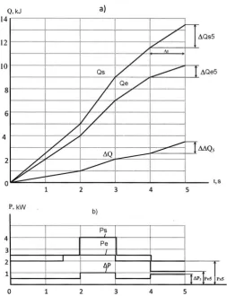
Let us consider one example of the method of diagnosing the condition of an energy element. Figs.1a and 1b depict the graphs of dependences of measured energy and calculated power on input, output and losses on elements since the time t.

Energy losses ΔQ(t) on the element are determined according to the following formula:

∆Q(t) = Qs(t) – Qe(t) (7)

Representative runtime t of the element is divided into N intervals of time with a step of Δt. The number of time

intervals N is determined according to the formula:

N = t/ Δt (8)

where Δt is the step of differentiation which depends on the shape of the curves Qs = f (t) and Qe= f (t) (for

Fig. 1. Graphs of the dependence of energy and power of elements on time t: a) Input energy – Qs(t), output energy – Qe(t) and losses – ΔQ(t);

b) Input power – Ps(t), output power – Pe(t) and losses – ΔP(t).

The values of increase in dependences Qs = f(t), Qe = f(t) and ΔQ = f(t) are determined in each of N time

intervals:

∆

Q



Q



Q

,

Q



0

;

i



1

...

N

∆

Q



Q



Q

,

Q



0

;

i



1

...

N

Fig. 1a depicts the fragments for determining the increase in energy: - on the input of the element – ΔQs5,

- on output of the element – ΔQe5,

- losses in element ΔΔQ5 in time interval i = 5.

The values of power on input Ps, on output Pe and losses ΔP in the element in N intervals (Fig.1b) are

determined under the assumption that in the time interval Δt the value of power does not change: - Psi = ΔQsi/Δt – power on the input of the element in time interval i;

- Pei= ΔQei/Δt – power on the output of the element in time interval i;

- ΔPi = Psi – Pei and ΔPi = ΔΔQi/Δt – power losses in element in time interval i.

Table 1 shows the results of the measurements and calculations of energy values (energy and power) of the element by time intervals.

Table 1. The results of measurements and calculations of the element’s energy values by time intervals Name of parameters Designation, and unit

of measurement

Value of parameters

Number of interval I 1 2 3 4 5

Value of measuring device on input

Value of measuring device on output

Qe, kJ 2 4 7 9 10

Losses in element ΔQ, kJ 0.5 1 2 2.5 3.5

Increase in energy on input ΔQs, kJ 2.5 2.5 4 2.4 2

Increase in energy on output ΔQ, kJ 2 2 3 2 1

Increase in energy losses in element

ΔΔQ, kJ 0.5 0.5 1 0.5 1

Power on input Ps, kW 2.5 2.5 4 2.5 2

Power on output Pe, kW 2 2 3 2 1

Power losses in element ΔP, kW 0.5 0.5 1 0.5 1

Step Δt, s 1 1 1 1 1

Current time t, s 1 2 3 4 5

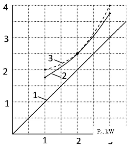
Figure 2 shows graphs of power dependences on input of element relating to power on its output – Ps= f(Pe).

Fig. 2. Dependence of the power on the element’s input on the power on the element’s output.

Ps= f(Pe): 1 – in a lossless element (for comparing actual and ideal modes);

2 – constructed based on the archived passport data of the element;

3 – constructed based on the results of measurements carried out on the element during the energy audit (for example, induction motor).

The number of time intervals with equal (or approximate) values of power on output of element Pe is then

determined. In this example, the number of time intervals with equal (or approximate) values of power on output of element Peis as follows (Table 2):

- when Pe= 1 kW; there is 1 interval; nj=1 = 1; - when Pe = 2 kW; there is 3 intervals; nj=2 = 3; - when Pe = 3 kW; there is 1 interval; nj=3 = 1,

P

kW

where nj is the number of work intervals of element with equal power























N

j

N

n

1

The portion of the element’s runtime at loads with similar (or approximate) values of power (as a ratio of the number of intervals with equal values of power to the number of intervals N) is determined.

The portion of the element’s runtime at power values:

- Pe= 1 kW: tp(1 kW) = nj=1/N=1/5=0.2;

- Pe = 2 kW: tp(2 kW) = nj=2/N=3/5=0.6;

- Pe = 3 kW: tp(3 kW) = nj=3/N=1/5=0.2.

Increase in energy losses in intervals with similar (or approximate) values of power on the output of the element

Pe in relation to the archived data of the power on the output of the element Pe is determined (Fig. 1; Table 2).

Table 2. The results of comparing archived data with data from calculations during energy audit of the element Data Ps(аrch), kW Pe(аrch),

kW

ΔParch, kW ΔР, kW nj, instances Proportion of runtime, tp ΔQ, kJ Archived (passport) data 1.75 2.5 3.75 1 2 3 0.75 0.5 0.75 - - - - - - - - - - - - Data Ps(meas), kW Pe(meas),

kW

ΔPΔPmeas, kW

ΔР, kW nj, instances

Proportion of runtime,

tp

ΔQ, kJ

During energy audit 2 2.5 4 1 2 3 1 0.5 1 0.25 0 0.25 1 3 1 0.2 0.6 0.2 0.25 0 0.25

In this example, increase in energy losses at time intervals with the same power values on the output of element

Pe has the following values (Table 3):

- The runtime of the element at Pe = 1 kW is tp(1 kW) = 0.2. Increase in power losses Δp is determined as the difference of values of power losses at the energy audit ΔPmeas and power losses according to archived data

ΔParch using the formula:

∆p = ∆Pmeas - ∆Parch = 1- 0.75 = 0.25 kW (10)

The actual power loss value exceeds the archived (passport) data by 0.25 kW. The value of the increase in energy losses ΔQ is determined according to formula:

∆Q = ∆p · ∆t · nj-1 = 0.25 · 1 · 1 = 0.25 kJ (11 - The runtime of the element at Pe = 2 kW is tp(2 kW)= 0.6.

The actual value of power losses and power losses according to archived passport data on element are equal. The increase in energy losses ΔQ at this load is zero;

- The runtime of the element at Pe= 3 kW is tp(3 kW)= 0.2. Increase in power losses Δp is:

∆p = ∆Pmeas = ∆Parch = 1- 0.75 = 0.25 kW (12)

The actual power loss value exceeds the archived (passport) value by 0.25 kW. The increase in energy losses ΔQ is determined according to the formula:

∆Q = ∆p · ∆t · nj-1 = 0.25 · 1 · 1 = 0.25 kJ (11)

The results of the energy audit have shown that at a load of Pe = 1 kW for a proportion of runtime tp(1 kW)= 0.2 and Pe = 3 kW for a proportion of runtime tp(3 kW) = 0.2, there is an increase in energy losses equal to ΔQ = 0.25 kJ.

III.

Conclusion

The developed method of diagnostics allows comparing the losses in elements depending on the load which varies with time and determining the increase in energy losses in the element. It also allows determining the proportion of runtime under equal loads, and the load creating the maximum energy loss, i.e., the most energy-consuming mode in which the deterioration of the element’s condition has the greatest effect on energy losses in this ETP.

REFERENCES

[1] Karpov,V., Yuldashev Z. 2010. Energy Efficiency. Finite Ratio Method. St. Petersburg: St. Petersburg´_{s State University of} Agriculture, 147 pp.

[2] Patent no. 2439500 RF. IPC О 01 Б 7/00. Multi-purpose module of an information and measuring system / Patent owner and applicant: St. Petersburg State Agrarian University, V. N. Karpov and Z. Š. Juldašev. Authors: V. N. Karpov, А. N. Halatov, Z. Š. Juldašev, А. V. Kotov, J. А. Starostenkov, V. А. Podberjozski; no. 2009140534/28; application 02.11.2009; published 10.01.2012. Bulletin no. 1. 8 pages: illustration.

[3] Kabanen T. and Karpov V. 2011. As an Addition to the Structural Theory of Optimizing Energy Efficiency in Consumer Systems. “Agronomy Research 2011”.

[4] Karpov V. Introduction to energy saving in an agro-industrial complex of undertakings. St. Petersburg State Agrarian University, St. Petersburg, 1999. 72 pages.

[5] Karpov,V., Gustsinski, A., Peiko,L, Zujev,V., Strubtsov, P. Finite relation method in an energy saving theory and in control of consumer's energy system. St. Petersburg State Agrarian University collection of research papers "Energy saving, useof electrical equipment and automatisation of processes in an agro-industrial complex", St. Petersburg, 2001. Pages 16-34.