Kernel-based Informative Feature Extraction via Gradient Learning

Kernel-based Informative Feature Extraction via

Gradient Learning

Songhua Liu1,2, Jiansheng Liu1, Caiying Ding1,3,4, Chaoquan Zhang1 1

College of Science, Jiangxi University of Science and Technology, Ganzhou, P. R. China 2

School of Computer Science and Technology, Xidian University, Xi’an, P. R. China 3

Center of Interdisciplinary, Lanzhou University, Lanzhou, P. R. China 4

Institute of Physics, Chinese Academy of Science, Beijing, P. R. China Email: [email protected]

Abstract—We consider the problem of feature extraction for kernel machines. One of the key challenges in this problem is how to detect discriminative features while mapping features into kernel spaces. In this paper, we propose a novel strategy to quantify the importance of features. Firstly, we derive an informative energy model to quantification of feature difference. Secondly, we move the features in the same class closer and push away those belong to different classes according to the model and derivate its objective function. Finally, gradient learning is employed to maximize this function. Experimental results on real data sets have shown the efficient and effective in dealing with projection and classification.

Index Terms—Kernel methods, nonlinear transformation, feature extraction, gradient learning.

I. INTRODUCTION

Obtaining important features with kernel machines is a challenging problem in classification tasks. It is also essential in exploratory data analysis, where the purpose is to map data onto a feature space for improved visualization. We are interested in methods that reveal discriminative features of the data sets. This can be achieved either by selection or by a transform from a large number of original features.

Feature selection methods [1-4] keep only useful features and discard others. Feature transform methods [5-9] construct new features out of the original features. However, algorithms that perform feature selection often lead to a combinatorial problem since all features need to be evaluated, but feature transform only need some criterion related to the performance of classifiers that would reflect the importance of a feature or a number of features. For this very reason, finding a transform might be easier than selection features. A further motivation for transforms is the ability to extract distributed relevant information across several original features, which produces a more compact representation than selection.

In this paper, we propose a novel method that aims to extract significant features by a new criterion within

kernel framework in conjunction with gradient learning, called kernel informative feature extraction (KIFE). The algorithm has some distinct characteristics: (1) It can extract high order statistics and nonlinear discriminative features; (2) this method can avoid the high time usage associated with eigenvalue decomposition in existing methods; (3) traditional criterion mutual information (MI) can be derived within the proposed KIFE framework, which helps users obtaining important features.

The rest of the paper is organized as follows. In Section II, we briefly summarize background and prior work. Then, the main algorithm is derived in Section III. Section IV presents the experimental results, and finally conclusions are drawn in Section V.

II. BACKGROUND AND PRIOR WORK

A. Notations

Let us denote by X the original feature set and by variableCthe class labels. xciis a sample in the input

space X, where c∈[1, ]C , N d

X∈R × andt∈[1,N_c],Nis the number of features in X,d is dimensionality of the features, Nc is the number of classes. We make use of a

dual notation for the featurexciin the input space, it is

written with a single subscript xi when its class is

irrelevant, index1≤ ≤i N. If the class is relevant, assume that we haveJcfeatures for cth class, we writexci, where

the class index 1≤ ≤c N_c , and the index within class1≤ ≤i J_c.

For a given kernel function :k X× →X R, the training featuresxi , 1≤ ≤i Jcare implicitly mapped to a feature

space F with usually high dimensionality. Let φ( )⋅ denotes the mapping fromXtoFandyi =φ( )xi ∈F, then

( , ) ( ), ( )

ij i j i j

k =k x x = φ x φ x (1)

B. Related Proir work

In general, feature extraction algorithms require certain criterions. Recently, research has been done on using different objective functions to address this problem. For example, Ref. [10] described a generalized discriminant Manuscript received September 29, 2010; revised December 7,

analysis (GDA) method, which depends on the eigendecomposition of the kernel matrix, which bears high computational complexity. Invoked by this problem, Ref. [11] used a low-rank approximation to a complete eigendecomposition of the kernel matrix. Recently, Ref. [12] proposed a kernel based nonlinear feature extraction, which transforms this problem to a kernel parameter learning problem. Ref. [13] presented a method for learning discriminative feature transforms using as criterion the MI between class labels and transformed features. Another recent paper by [14] employed conditional information and information losses to extract main features in input features.

However, the similarity measure in many of these papers depends only to the Euclidean measure. When samples have equal Euclidean distances to training samples, the kernel mapped the samples into the same vectors. This may not perfectly fulfill the purpose of classification-oriented feature extraction. On the other hand, MI according to Shannon’s definition is computationally expensive.

III. THE ALGORITHM FOR THE KIFE

In this section, we describe KIFE as Algorithm 1, which trained with training data Xand its class label set

C. After the kernel matrix is obtained, the algorithm has three stages. In the first stage, we define a function to quantification of the feature difference. In the second stage, we derive the objective function for feature extraction. Then, gradient learning is used to optimize the objective function and find the optimal coefficient matrix.

A. Detailed Description of Our Main Algorithm

In the first stage of KIFE, we propose an informative energy model. The main idea is that we quantify the difference between features according to their graph energy [15]. Our goal is to transform the kernel space so that the distance in the transformed space correlated with the difference of the labels of features. So, we need to define informative energy for our method.

The graph energy in [15] is defined as

2

1

1

( ) ( , 2 ) ( , )

N

j j i j i

i

E G x x I H x x

Z

σ σ

=

=

∑

−

where 2

2

1

( , ) exp

2 T

G yσ y y

σ

⎛ ⎞

= _⎜− _⎟

⎝ ⎠ the Gaussian kernel function, σj∈σ is the kernel width parameter, H is an

indicator function, 2

1 1

( , 2 )

N N

j i

j i

Z G x x σ I

= =

=

∑∑

− is a

normalization variable. The Energy value is 1 when the featurex_iandx_jare in the same class, otherwise 0 when they are in the different class.

For the feature y_ci =φ(x_ci) in the kernel space, we define its informative energy according to the graph energy model. The main difference is that we consider each feature in the kernel space as a particle, and pull or push other particles in this space. This means that the

resultant effect of a particle is the sum of the separate effects between the same class and the different classes. For each feature we defined two informative energy function: similar and dissimilar energy. For the features in the same class, the similar energy is computed as follows

2

1

1

( ) ( , 2 )

c

J

c ci cj ci

j

E y G y y I

N = σ

=

∑

− (2)

where I is the identity matrix.

Then the dissimilar energy considering features between different classes is computed as

2

1 1

1

( ) ( , 2 )

p c J

N

p c ci pl ci

p l

E y G y y I

N σ

≠

= =

=

∑∑

− (3)

These two energy functions vary between 0 and 1. A highEcindicates that two features in the same class are

quite similar. But a lowEp c≠ indicates that two features in

the different class are quite different. We can use these two values to quantify the difference between any feature pairs.

In the second stage, we derive the objective function for feature extraction. In order to improve the performance of the projection and classification, we need to move the features in the same class as close as we can. Meanwhile, the features belong to different classes are push away as far as possible.

As mentioned above, we have the simple idea that E y_c( _ci) should as large as possible, andE_{p c≠} (y_ci)should be as small as possible. This can ensure the separation between the different classes and the aggregation within the same class. Then, the total resultant effect can be computed as

1 1

1

( ) ( ) (1 ) ( )

c c

N J

c ci p c ci

c i

E y E y E y

N = = α α ≠

=

∑∑

− − (4)

where

2 2

1

1

1 1

c

N p

c

p p c

J J

k k

α =

≠

⎡_{⎛ ⎞ ⎛ ⎞} ⎤

⎢ ⎥

= _⎜ − _⎟ + _{⎜ ⎟}

+ +

⎢⎝ ⎠ ⎝ ⎠ ⎥

⎣

∑

⎦

presents the

effects from the same class and the different class, kis the number of neighborhood of yci . The first term

ofαmeans effects of all features toyci, the second term

means effects of other features to yciexcept the features

in classc.

However, yci =φ(xci)cannot be computed explicitly. So we transform it to a coefficient matrix learning problem. In the kernel space, we can projectyciinto a new

feature space, and define this space asFfor simplicity. Owing to the kernel trick, we can modifyycias following

1 1

, ( ) ( , )

c

J C

ci ci st st ci

s t

y vφ x β K x x

= =

whereK is the kernel matrix, K x x( ,_{i j})=k_ij ,β is the coefficient when project the original y_ci onto the direction v . In this form, we can compute the variablesypl−yciin (2) and (3) as

(

)

,

( , ) ( , )

pl ci s ci t ci

s t

y −y =B⎛_⎜ K x x −K x x ⎞_⎟

⎝

∑

⎠ (5)

where elements ofBis constructed byβ as well as the kernel matrix.

In the third stage, we need to employ optimization methods to maximize the objective function (4). There are many algorithms we can used, such as traditional quotient method of GDA, but it bears eigendecomposition problem, which may result in high computational complexity. Recently, semi-definite programming (SDP) is widely used for this optimization [16]

. But it is also quite time consuming when the number of features is large, so we adopt gradient ascent algorithm.

Substituting (5) into (4), we can transform the feature

ylearning problem to the coefficient matrixBlearning problem as follow

1 1

1

( ) ( ) (1 ) ( )

c c

N J

c ci p c ci

c i

E B E y E y

N = = α α ≠

=

∑∑

− − (6)

Maximizing (6) creates a transformed feature space with wide separation of the different class and better clustering of the same class. The gradient for the objective function is

1 1

( ) ( )

1

(1 ) c c

N J

p c ci c ci

c i ci ci

E y

E y E

B N α y α y

≠

= =

∂ ∂

∂

= − −

∂

∑∑

∂ ∂ (7)

In Eq. (7), the computation of c( ci) ci

E y y

∂

∂ by chain rule is

c c ci

ci

E E y

B y B

∂ ∂ ∂

=

∂ ∂ ∂ and

( )

p c ci

ci

E y

y ≠

∂

∂ is

p c p c ci

ci

E E y

B y B

≠ ≠

∂ ∂ ∂

=

∂ ∂ ∂ ,

where c ci

E y

∂ ∂ is

2

2 1

( )

1

( , 2 )

c

J

cj ci

c

cj ci

j ci

y y E

G y y I

y N = σ σ

− ∂

= −

∂

∑

(8)

and p c

ci

E y

≠

∂

∂ is

2

2 1 1

( )

1

( , 2 )

p c J

N

p c pl ci

pl ci

p l

ci

E y y

G y y I

y N σ σ

≠

= =

∂ −

= −

∂

∑∑

(9)

and yci B ∂

∂ is

( , )

ci

s ci s

y

K x x B

∂ =

∂

∑

(10)

substituting (8) (9) and (10) into (7), we can obtain the gradient of the objective function.

Maximizing the objective function (6) using gradient ascent algorithm, we can get the final coefficient matrix B , which can be used for classification and projection.

Finally, the KIFE is briefly described by the following

Algorithm 1. KIFE

Input: Training data set X , class label setC , and integerk.

Output: A coefficient matrixB. // Initialization

Compute the kernel matrixK =(kij)1≤ ≤i N,1≤ ≤j N.

// The first stage

Get the graph energy of each feature according to (2) and (3).

// The second stage

Construct the objective function according to (6). // The third stage

Run the gradient learning optimization method according to (7), (8), (9) and (10).

Return the final coefficient matrixB.

In this section we will explain how the gradient of the objective function (6) provides information on the geometry and statistical variables to predicting the class label given a new feature. Our KIFE is motivated by the following idea: the gradient is a local concept as it measures local changes of the objective function (6). In the optimization processing for the objective function, we found thatBvarying with the gradients of (6) as follows

1

r r

E

B B

B η

+

∂

= +

∂

whereris the learning step,ηis learning rate, these two parameters can be obtained using the cross-validation method.

We present visualization experiment with synthesized data. In this example we learn a nonlinear projection from a high-dimensional feature space onto a discriminative direction for visualization purposes, specially to visualize classification ability. The data is non-Gaussian densities. It is three-dimensional, and two classes. Class one has 200 samples from a bimodal Gaussian distribution, with centers at (1,0,0) and (-1,0,0). Class two has 200 samples, also from a bimodal Gaussian distribution, with centers at (0,1,0) and (0,-1,0).

Since we have two classes, KIFE is able to produce a two-dimensional projection. In this example, GDA was used as the initial state to learn the KIFE-projection. The result is presented in Figure 1. Using the gradient ascent algorithm, KIFE can converge to the global optimum in 16 iterations, which now exhibits much better separation.

(a) The origianl data (b) Before learning (c) After learning

Figure 1. Projection results on synthesized data.

one, the symbol “×” is those features in class two. Figure 1(b) shows the status of the original features in the input space. After KIFE learning, the final status is presented in Figure 1(c).

From Figure 1 we can found out several characteristics of this example: (1) features in the same class are clustered; (2) features in the different class are pushed away.

Recall that informative energy function (2) and (3) can reflect the distance of features in the kernel space. The central quantity is an estimate of the gradient of the difference of features, which is controlled by those neighborhoods. So we find kneighborhoods ofyci, those

in the same class are moving closer and in the different class are push away. From the view of nearest neighborhood (NN), this can improve the performance of classification and projections. Then our KIFE can be viewed as a graph, each node is the feature in transformed space and is connected with its nearest neighborhood.

B. Relation to MI criterion

We show that different setting of the trade-off parameter α will lead to special versions of KIFE algorithm, which are highly related to the popular criterion MI.

We have the following theorem:

Theorem 1. Letα in (6) a constant, whenk=N−1, then our objective function (6) is the same as MI criterion. Proof. In [13], MI is computed by Renyi entropy, according to definitions in our method, we can rewrite the MI computed in [13] as

2

IN ALL BTW

MI=V +V − V (11)

where the quantities appearing in (11) are as follows

2 2

1 1 1

1

( , 2 )

p p c J J

N

IN pk pl

p k l

V G y y I

N = = = σ

=

∑∑∑

− (12)

2

2 2

1 1 1

1

( , 2 )

c

N N N

p

ALL k l

p k l

J

V G y y I

N

N = = = σ

⎛ _{⎛ ⎞} ⎞ ⎜ ⎟ = _{⎜ ⎟} − ⎜ _{⎝ ⎠} ⎟ ⎝

∑

⎠

∑∑

(13) 2 2

1 1 1

1

( , 2 )

p

c J

N N

p

BTW pj k

p j k

J

V G y y I

N

N = = = σ

=

∑ ∑∑

− (14)

substituting (12), (13) and (14) into (11), we can obtain the MI values.

In our KIFE, the objective function is

1 1

1

( ) ( ) (1 ) ( )

c c

N J

c ci p c ci

c i

E B E y E y

N = = α α ≠

=

∑∑

− − where 2 2 1 1 1 1 c N p c p p c J J k k α = ≠ ⎡_{⎛ ⎞ ⎛ ⎞} ⎤ ⎢ ⎥ = _⎜ − _⎟ + _{⎜ ⎟} + + ⎢⎝ ⎠ ⎝ ⎠ ⎥ ⎣

∑

⎦ .

When we consider allN−1features in the kernel space as neighborhoods of certain feature yci , this

meansk=N−1. Then, we can computed the parameter in (6) as

2 2

1

2

1 c Nc p c

p p c

J

J J

N N N

α =

≠

⎛ ⎞

⎛ ⎞

= +_{⎜ ⎟} + _{⎜ ⎟} −

⎝ ⎠

∑

⎝ ⎠ (15)

substituting (15) into (6), we rewrite (6) as

(

1 2 3

)

2

1 ( )

E B E E E

N

= + +

where 1

E , 2

E , 3

E are computed as follows, for convenient, we write_G(⋅ − ⋅_{, 2}σ2_I)

asG(⋅ − ⋅)

1

1 1 1

( )

c c c

N J J

cj ci

c i j

E G y y

= = =

=

∑∑∑

−

2 2

1 1 1 1 1

2

1 1 1 1

( ) ( )

( ) ( )

p

c c c c

p

c c c

J

N J J N

c

cj ci pl ci

c i j p l

p c J

N N J

P

cj ci pl ci

p c i l

p c

J

E G y y G y y

N

J

G y y G y y

N = = = = = ≠ = = = = ≠ ⎛ ⎞ ⎛ ⎞ _{⎜ ⎟} = _{⎜ ⎟ ⎜} − + − _⎟ ⎝ ⎠ ⎜_⎝ ⎟_⎠ ⎛ ⎞ ⎛ ⎞ + _{⎜ ⎟} ⎜_⎜ − + − ⎟_⎟ ⎝ ⎠ _{⎝ ⎠}

∑

∑ ∑

∑∑

∑

∑ ∑

∑

3

1 1 1 1 1

2 ( ) ( )

p

c c c c J

N J J N

c

cj ci pl ci

c i j p l

p c

J

E G y y G y y

N = = = = = ≠ ⎛ ⎞ ⎜ ⎟ = − _⎜ − + − _⎟ ⎜ ⎟ ⎝ ⎠

∑ ∑ ∑

∑∑

For _E1

, it computes informative energy in the same class, this is the same as VIN in (12) except the

normalization factor 1₂

N . So,

1 2 1 IN E V N = . For 2

E , we can find that

1 ( ) c J cj ci j

G y y

=

−

∑

computes

informative energy for class (c c≠ p), the other term

1 ( ) p J pl ci l

G y y

=

−

∑

computes informative energy for class

( )

into one term without considering the class label. ThenE2can be modified as

2

2

1 1

2

1

( , 2 )

c

N N N

p

k l

p k l

J

G y y

N

E σ I

= = =

⎛ _{⎛ ⎞} ⎞

⎜ _{⎜ ⎟} ⎟ −

⎜ _{⎝ ⎠} ⎟

=

⎝

∑

⎠

∑∑

For 3

E ,

1 1 1

( ) ( )

p

c c J

J N

cj ci pl ci

j p l

p c

G y y G y y

= = =

≠

− + −

∑

∑∑

computes

informative energies for class c c( ≠ p) and class p p( ≠c) , they can be merged into one term

as 2

1 1

( , 2 )

c

J N

k ci

i k

G y y σ I = =

−

∑∑

. ThenE3 can be modified as

2 3

1 1 1

2 ( , 2 )

p

c J

N N

p

pj k

p j k

J

E G y y I

N σ

= = =

= −

∑ ∑∑

−

substituting_E1

,_E2

and_E3

into

(

1 2 3

)

2

1 ( )

E B E E E

N

= + + ,

we obtain

( ) _{IN ALL} 2 _BTW

E B =V +V − V

CompareE1,E2andE3with (12), (13) and (14), we know that whenk=N−1, E B( )is equal to MI.

Then, MI criterion is a special case of our objective function (6). □

As mentioned above, we can get the same criterion as MI, the main difference is that we can change the parameter k to obtain the high performance of classification and projections, and this is the same idea as NN algorithms. However, we cannot necessarily hope to preserve the quality of quantification of difference of features, we may sacrifice its power to obtain corresponding gains in classification accuracy and computational efficiency. Experimental results show that KIFE appears promising in the contexts of classification and projections. This feature is especially desirable for kernel-based methods such as those yield very large kernel matrices for important feature extraction.

C. KIFE for Dimension Reduction via Gradient Learning

In this section, we show how to using KIFE for dimension reduction. The main problem in the kernel space is that its dimensionality depends on the number of features. So we need reduce the dimensionality for visualization and complexity reduction. Here, we employ the gradient learning algorithm [17]. It has some merit suit for our model: (1) it is simple to run; (2) it holds for Euclidean spaces as well as the manifold setting.

Firstly, we define graph Laplacian

1 2 1 2

L= −I D− WD− (16)

where I is the identity matrix, ii ij j

D =

∑

W ,Wij is a

similarity metric between two pointsyiandyj.

In literature [17], they defined a regression function to computeWij. Here, we propose a novel similarity metric

according to the difference quantification function (4)

(

) (

)

2

2 ₁ 2

1 2

( , )

( ) ( )

exp

ij E i j

i j i j

i j

W W y y

E y E y y y

y y

σ σ

=

⎛ _{− ∇ + ∇ ⋅ −} ⎞

⎜ ⎟

= _⎜− − _⎟

⎜ ⎟

⎝ ⎠

where ( )_i i

E E y

y ∂

∇ =

∂ ,

1

σ andσ2

are parameters.

In the similarity metricWij,

2

i j

y −y represents the local geometry of the marginal distribution and the second term pastes together gradient estimates between neighboring features.

The main differences between the metric in [17] and ours are: (1) the first term in [17] is used in unsupervised dimension reduction such as Laplacian eigenmaps or diffusion maps, but we can use it considering its class label; (2) the second term in [17] can be interpreted as a first order Taylor expansion leading to the following approximation

(

) (

)

1

( ) ( ) ( ) ( )

2 ∇E yi + ∇E yj ⋅ yi−yj ≈E yi −E yj .

But ours can be computed explicitly according to the function (4); (3) the method in [17] is defined in the input spaceX, but ours is defined in the feature spaceF.

Once the similarity metricWij is obtained, we can

compute the graph Laplacian according to (16). Then, dimension reduction is achieved by projection onto a spectral decomposition of the matrixL.

The pseudo-code of KIFE for dimension reduction is in the following form.

Algorithm 2. KIFE for dimension reduction using gradient learning

Input: Training data set X , class label setC , and integerk.

Output: A dimension reduction matrix. // Initialization

Give an integerD, it represent the final dimension. // The first step

Compute the similarity metricW_ij. // The second step

Compute the graph LaplacianLaccording to (16). // The third step

Run decomposition onL. // The fourth step

Pick the topDeigenvectors.

Return the final dimension reduction matrix.

IV. EXPERIMENTAL RESULTS

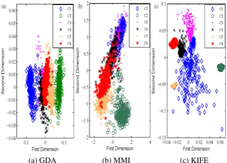
(a) GDA (b) MMI (c) KIFE

Figure 2. Projection results on Statlog. the algorithms 1 and 2 of Section III. The algorithm 1 is

mainly used as a preprocessing for classification tasks. The algorithm 2 is used for dimensional reduction.

In this section, we evaluated KIFE on real benchmark data sets of varying size and difficulty. The Phoneme set is available with maximize mutual information (MMI) algorithm in [13]. The rest of data sets are cited from the UCI data sets (http://archive.ics.uci.edu/ml/). The data sets and some of their characteristics are presented in Table 1.

In Table 1, Training/Sampling means that the number of the original features/the number of features sampling for training,D is the dimension reduction number for projection, dis the original dimension of the data set.

We will conduct two experiments: dimension reduction for projection and classification. We compare KIFE with two existing methods. In order to facilitate the comparison, we duplicate the GDA in [10] and the MMI in [13]. The kernel widthσis selected by the method in [13].

A. Visualization of Class Separation

In the first experiment, we illustrate a projection from 36-dimensional Statlog feature space onto two. We employ algorithm 2, the extension of KIFS, to perform dimension reduction. Two existing dimension reduction methods are duplicated for comparison: GDA and MMI. GDA uses the label information to find informative projection such that the separation of data of different classes can be maximized and data of same classes should be highly aggregated. To that end, GDA tries to maximize the inter-class scatter matrix and minimize the intra-class scatter matrix simultaneously. However, GDA suffers from the singular problem when dealing with high-dimensional data, and its dimension reduction number is controlled by the number of classes. MMI is a non-parametric learning method. Promising performance of MMI have been shown in [13] for classification, but it is mainly used as a linear projection algorithm. Since our quantification method is based on a energy function which is similar to MMI, we empirically compared our method with GDA and MMI.

The Statlog is the Statlog satellite image database from UCI Machine Learning Repository. It has 4435 features for training, and 2000 for testing. Its dimensional is 36 and the number of classes is six. For dimension reduction task, we randomly sample 1800 from the training data and use total testing data. Those six classes are according to the label in Figure 2, where C1 represents red soil, C2 is cotton crop, C3 is grey soil, C4 is damp grey soil, C5 is soil with vegetation stubble, and C6 is very damp grey soil. This data is one of the many sources of information

available for a scene. The interpretation of a scene by integrating spatial data of diverse types and resolutions including multispectral and radar data, is a difficult task. The GDA projection is presented in Figure 2(a), MMI-projection in Figure 2(b), and KIFE-MMI-projection in Figure 2(c).

From the Figure 2, we observed that GDA separates C1, C2 and C5 very well. MMI separates C2 and C5 but places other four classes almost on the top to each other. The criterion of KIFE is a combination of representing each class as compactly as possible and as separated from each other as possible. Figure 2(c) has achieved this: all classes are represented as quite compact clusters. But we should note that C1 is scattered and has small cross parts with other classes. We can obtain the following conclusions: (1) GDA can separate the red soil, cotton crop and vegetation stubble. The other three soil features are overlapping with each other. (2) MMI can separate the cotton crop and vegetation stubble, but the other four soil features cannot be separated well. (3) KIFE firstly separate the cotton crop from other soil features, the other four soil features are separate well except the red soil. This means that the gradient information in the transform processing may be useful for classification problem.

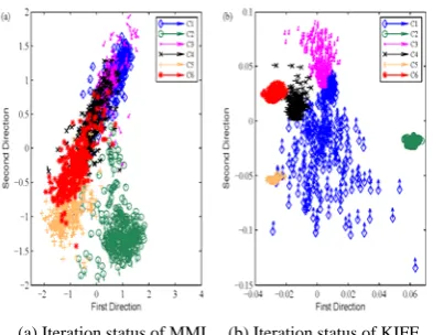
In order to evaluate how the features transform according to KIFE, we plot the gradient of each feature until the coefficient matrix is obtained. In this setting, linear discriminant analysis (LDA) is used as an initial state of MMI, and GDA for KIFE. We also used LDA as an initial state of KIFE, experimental result has shown that our method is not sensitive to the initialization, but need 41 steps to converge to the optimal solution.

Figure 3 shows the iteration status of 24 steps using gradient learning. Figure 3(a) shows the gradient learning about MMI, we can find out why MMI cannot separate other four classes. The direction of C3 has no regular arrangement, and it overlaps with C1. However, KIFE shows better results. All classes have better clustering performance except C1. From the direction of C1 in figure 3(b), we find out that features in C1 have the tendency toward the within class center, and C1 has little overlapping area with C3.

TABLE I.

CHARACTERISTICS OF THE DATA SETS AND PARAMETER SETTINGS

Data Training/Sampling Testing/Sampling Nc/d/D

Iris 150/105 150/45 3/4/2

Statlog 4435/1800 2000/2000 6/36/2

Letter 16000/2000 4000/1500 26/16/8

(a) Iteration status of MMI (b) Iteration status of KIFE

Figure 3. Iteration status of 24 steps using gradient learning.

Figure 4. Influence of the k values. This result is useful when the feature is difficult to

classify. We can predict its potential class label according to its move direction in feature space.

B. Classification Results

In the second experiment, we applied our feature extraction method to improve the classification of nearest neighbor algorithm knnclassify in Matlab.

We must first determine k, the number of the nearest neighbor to construct the objective function. We selected thekfrom {3,5,7,9,11} according to their classification performance. We averaged over 100 runs with random sampling of Landsat data set according to Table 1. Figure 4 shows the interaction between the value ofkand the accuracy of nearest neighbor algorithm.

It can be observed that we can obtain high classification performance when k=5. Therefore, we assignedk=5.

In order to evaluate whether our KIFE feature extraction method actually results in a new space that characterizes the difference between features better, we perform our algorithm using other data sets showed in Table 1. Iris is perhaps the best known data used in the pattern recognition literature. The data set contains three classes of 50 instances each, where each class refers to a type of iris plant. One class is linearly separable from the other two, the latter one are not linearly separable from each other. For this small sample, we use cross-validation to random select features for training and testing. The Phoneme is widely used resource for research in speech recognition. It contains 20 classes of 20 dimensional. The Letters is a database of character image features. It contains 26 capital letters, we randomly sample 2000 from 16000 for training and 1500 from 4000 for testing. Detailed description is listed in Table 1, we run experiments 10 runs, the performance of these methods are show in Table 2.

On the other hand, we report the computation time of the KIFE algorithm, as KIFE avoids the eigendecomposition of GDA. For MMI and KIFE, we terminate the algorithms when the iteration step is up to 24. We can observe that KIFE has the similar computational complexity, and they are all superior to

GDA. However, the classification performance of GDA is superior to MMI, because GDA can extract nonlinear features. KIFE combines the merits of these two algorithms, so it shows high performance on these data sets.

The above experiments show that it may be beneficial to combine KIFE with classifiers, because KIFE can extract important features and can be used for dimension reduction.

Other advantages of our algorithm are

• KIFE can be easily extended to dimension reduction based on gradient learning. It can be used in many applications, such as in [18-20].

• It can extract high order statistics and nonlinear statistics from data sets. Contrary to GDA and MMI, our method holds both for Euclidean and manifold setting.

• Computational efficiency. Our approach naturally draws advantages from gradient ascent implementation. But the extension of KIFE for dimension reduction needs eigendecomposition, which can be considered as a preprocessing step for classification or regression tasks.

• Extraction ability. The important feature extracted by our method can improve the visual ability of projection, and can be used for classification task when the number of features is large.

The informative energy function can be used as a quantification of feature difference. We expect that this function can be used in bioinformatics in future work.

V. CONCLUSION

A novel algorithm, KIFE, for feature extraction is presented. The algorithm works in an iterative fashion and the final coefficient matrix is obtained during successive iterations. Experimental shows that KIFE has lower time complexity than GDA, and it is superior to MMI in classification performance.

TABLE II.

TEST PERFORMANCE OF PROJECTION ALGORITHMS(%/S)

Iris Statlog Phoneme Letters

Another algorithm for dimension reduction is also evaluated, which is an extension of KIFE. This can be considered as a preprocessing step for classification. Nevertheless, the fascinating idea of using our approach is that we build a connection between feature extraction and gradient learning.

In future work we intend to apply the proposed method to larger data sets, especially for bioinformatics. We also want to modify our algorithm to parallel implementations. In addition, how gradient of the objective function influence the performance of the classifiers is an interesting topic.

ACKNOWLEDGMENT

The authors wish to thank Editor and referees. This work was supported by the Doctoral Foundation of Jiangxi University of Science and Technology, Jiangxi Educational Committee Foundation for Youths, National Natural Science Foundation of China (61070137, 60702063).

REFERENCES

[1] M. Yang, F. Wang, P. Yang. “A novel feature selection algorithm based on hypothesis-margin”, Journal of Computers, 2008, 3(12): 27-34

[2] L. Li, M. Li, Y. Lu, Y. Zhang. “A new multi-objective genetic algorithm for feature subset selection in fatigue fracture image identification”, Journal of Computers, 2010, 5(7): 1105-1111

[3] I. Rodriguez-Lujan, R. Huerta, C. Elkan, and C. S. Cruz. “Quadratic programming feature selection”, Journal of Machine Learning Research, 2010, 11: 1491-1516

[4] S. Zhu, D. Wang, K. Yu, T. Li. “Feature selection for gene expression using model-based entropy”, IEEE/ACM Transactions on Computational Biology and Bioinformatics, 2010, 7(1): 25-36

[5] F. Oveisi, A. Erfanian. “A minimax mutual information scheme for supervised feature extraction and its application to EEG-based brain-computer interfacing”, EURASIP Journal on Advances in Singnal Processing, 2008

[6] K. Lee. “Exploration on feature extraction schemes and classifiers for shaft testing system”, Journal of Computers, 2010, 5(5): 679-686

[7] K. Torkkola, W. M. Campbell. “Mutual information in

learning feature transformations”, Proceedings of the 17th International Conference on Machine Learning, Stanford, USA, 2000, 1015-1022

[8] U. Ozertem, D. Erdogmus, R. Jessen. “Spectral feature projections that maximize Shannon mutual information with class labels”. Pattern Recognition, 2006, 39: 1241-1252

[9] X. Yuan, B. Hu. “Robust feature extraction via information theoretic learning”, Proceedings of the 26th International Conference on Machine Learning, Montreal, Canada, 2009, 1193-1200

[10]G. Baudat, F. Anouar. “Generalized discriminant analysis using a kernel approach”, Neural Computation, 2001, 12: 2385-2404

[11]A. R. Teixeira, A. M. Tome, E. W. Lang. “Feature

extraction using low-rank approximations of the kernel matrix”, Proceedings of the 5th International Conference on Image Analysis and Recognition, Lecture Notes In Computer Science, Povoa de Varzim, Portugal, 2008, 5112: 404-412

[12]M. Wu, J. Farquhar. “A subspace kernel for nonlinear feature extraction”, Proceedings of the 20th International Joint Conference on Artifical Intelligence, Hyderabad, India, 2007, 1125-1130

[13]K. Torkkola. “Feature extraction by non-parametric mutual information maximization”, Journal of Machine Learning Research, 2003, 3: 1415-1438

[14]R. Kamimura. “An information-theroretic approach to

featuren extraction in competitive learning”, Neurocomputing, 2009, 72: 2693-2704

[15]X. Zhu, Z. Ghahramani. “Learning from labeled and

unlabeled data with label propagation”, Technical Report CMU-CMLD-02-107, Carnegie Mellon University, Pittsburg, PA, 2000

[16]C. Shen, H. Li, M. J. Brooks. “Feature extraction using sequential semidefinite programming”, Proceedings of the 9th biennial Conference of the Australian Pattern Recognition Society on Digital Image Computing Techniques and Applications, Glenelg, Australia, 2007, 430-437

[17]Q. Wu, J. Guinney, M. Maggioni, S. Mukherjee. “Learning gradients: predictive models that infer geometry and statistical dependence”, Journal of Machine Learning Research, 2010, 11: 2175-2198

[18]J. Cai, H. Wang, D. Zhou. “Gradient learning in a

classification setting by gradient descent”, Journal of Approximation Theory, 2009, 161: 674-692

[19]N. D. Ratliff, J. A. Bagnell. “Kernel Conjugate Gradient for Fast Kernel Machines”, Proceedings of the 20th International Joint Conference On Artifical Intelligence, Hyderabad, India, 2007, 1017-1022

[20]G. Tzimiropoulos, V. Argyriou, S. Zafeiriou, T. Stathaki. “Robust FFT-based scale-invariant image registration with image gradients”, IEEE Transactions on Pattern Analysis and Machine Intelligence, 2010, 32(10): 1899-1906

Songhua Liu received his PhD degree in Technology of Computer Application from Xidian University, Xi’an, China, in 2011. He is currently a lecturer in the College of Science in Jiangxi University of Science and Technology, Ganzhou, China. His research interest covers machine learning and intelligent information processing, image processing, machine learning, bioinformatics.