Vol. 04, Issue 08 (August. 2014), ||V2|| PP 12-20
Simulation Studies of Bioreactor Using Artificial Neural Network
Based Direct Inverse Method
Ballekallu Chinna Eeranna
Dept.of petroleum Engineering, Lords institute of engineering and Technology Hyderabad,
Abstract: In this paper presents about control of Bioreactor useing Artificial Neural Network. bioreactor has become an active area of research in recent years. This is partially attributable to the fact that bioreactors can be extremely difficult to control. Their dynamic behavior is invariably non-linear and model parameters vary in an unpredictable manner. Accurate process models are rarely available due to complexity of the underlying biochemical processes. A feedback controller is needed to account for disturbances and time-varying behavior. Neural network based model predictive controller designed for the control of bioreactor. In the first step the neural network model of bioreactor is obtained by levenburg- marquard training the data for the training the network generated using mathematical model of bioreactor.
Keywords: Neural network direct inverse, predictive control, Bioreactor,Productivity and Dilution rate.
I. INTRODUCTION
A control system is defined as a system in which deliberate guidance or manipulation is used to achieve a prescribed value of a variable. In the last two decades, a new direction to control has gained considerable attention. This new approach to control is called „Intelligent control‟. The term „conventional control‟ refers to theories and methods that are employed to control dynamic systems whose behavior is primarily described by differential and difference equations. The term „intelligent control‟ addresses to more general control problems. It may refer to systems, which cannot be adequately described by a differential equations framework. There are three basic approaches to intelligent control knowledge-based experts systems, fuzzy logic and neural networks.
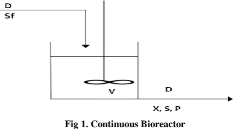
II CONTINUOUS BIOREACTORS
In most of the continuous fermentation processes, one of the output variables is chosen as the controlled variable (biomass concentration or product concentration) and its estimated optimal open loop profile of a constant set point is tracked. A continuous stirred tank fermenter (CSTF) is an ideal reactor, which is based on the assumption that the reactor contents are well mixed.
Fig 1. Continuous Bioreactor
3. PROBLEMS WITH THE CONVENTIONAL CONTROLLER
result in a total of 5 steady states (three stable and two saddle points) even though a sufficient control action is present.
4. CONTROL OF BIOREACTORS USING NEURAL NETWORK
The inherent non-linearity of the fermentation process often renders control difficult. Neural network has become popular tool for modeling and control of dynamic process, demonstrating the ability of handling non-linearity. Many neural network controllers are of the rule-based type where the controller‟s output response is described by a series of control rules.
The unique features of this neural network control technique include:
A wide operation range for handling a non-linear process.
Robustness for dealing with random disturbance and possible system parameter Drafting.
Relatively simple implementation.
In the present work, neural network control is designed and evaluated for the continuous bioreactor with one input and one output to overcome the control problems associated with linear P1 controller due to the input multiplicity.
5. MATHEMATICAL MODELLING OF A CONTINUOUS BIOREACTOR
A schematic of a continuous bioreactor is shown in figure.1-We assume that the bioreactor has constant volume, its contents are well mixed, and the feed is sterile. The dilution rate D and the feed substrate concentration Sf are available as manipulated inputs. The effluent cell-mass or biomass concentration X,
substrate concentration S and product concentration P are the process state variables. In ethanol production, for example, X, Y, and P represent yeast, glucose, and ethanol concentrations, respectively.
5.1 MODEL DERIVATION:
The dynamic model is developed by writing material balances on the biomass (cells), the substrate (feed source for cells) and the product. Biomass grows by feeding on the substrate results in generation of product.
Biomass Material Balance
We write biomass material balance as: Rate of accumulation = i/p – o/p + generation d(VX)/dt=FXf – FX + Vr1 (1)
Substrate Material Balance:
The substrate material balance is written as: Rate of accumulation =i/p – o/p – consumption d(VS)/dt = F Sf – FS – Vr2 (2)
Product Material Balance:
Finally, the product material balance is written as: Rate of accumulation =i/p – o/p + genrn
D (VP)/dt = 0 – F P + Vr3 (3)
The reaction rate (mass of the cells generation/Volume/time) is normally written in the following form: r1 = µX (4)
As yield Y = r1/r2, r2 = r1/Y
And hence r2 = µ X/Y (5)
Similarly r3 = (αµ+β) X (6)
Defining F/V as D, the dilution rate, and assuming biomass feed concentration as Zero, we find: dX/dt = - D X +µ X
dS/dt = D Sf – Ds – µX/Y
dP/dt = - D P + (α µ+ β) X
Finally, the model equations can be written as;
X = -DX + µX (7)
S = D (Sf - S) – µX/Y (8)
P = -DP + (αµ +β ) X (9)
This unstructured model can describe a variety of fermentations. Because Y, and P are assumed to be independent of the operating conditions, above model is called a constant yield model. The specific growth rate model is allowed to exhibit both substrate and product inhibition:
1 2/
/
1
K
S
S
K
S
P
P
m m m
(10)Model equation of the system on which the study is based:
In practice, the model parameters in equations (7)-(10) are chosen to fit experimental data (Munack and Thoma, 1986; Enfors et a!., 1990). If the bioreactor deviates significantly from the operating conditions where the data was collected, the model parameters previously determined may no longer be valid. The cell-mass yield Y and the maximum specific growth rate tm tend to be especially sensitive to changes in the operating conditions. From a process control perspective, these two model parameters can be viewed as unmeasured disturbances because they may exhibit significant time-varying behavior. Many types of fermentations can be modeled by choosing the model parameters appropriately . For instance, the product is totally growth-associated if a α ≠ 0, β = 0, totally non growth-associated if a = 0, β≠ 0, and a combination of the two if α ≠ 0, β≠0. Simple Monod kinetics (Johnson, 1987) can be obtained by setting Pm = K1 =α „c. In many fermentations such as penicillin production, cell growth is inhibited by high substrate concentrations so that 0 < K1 < cc. If the growth rate approaches zero at high product concentrations then 0 <Pm < α.
Nominal model parameters and operating conditions used throughout the study are listed below:
Variable Nominal value
Y 0.4 g/g
Α 2.2 g/g
Β 0.2 h-1
µm 0.48 h-1
Pm 50 g/1
Km 1.2 g/1
K1 22 g/1
Sf 20 g/1
If the biomass and substrate are of negligible value when compared to that of the product, the productivity Q can be defined as the amount of product cells produced per unit time:
Q = DP (11)
6. DESIGN OF A DIRECT INVERSE NEURAL NETWORK CONTROL
Conceptually, the most fundamental neural network based controllers are probably those using the “inverse” of the process as the controller. The simplest concept is called direct inverse control.
The principle of this is that if the process can be described by:
y(t +1) =g(y(t),…… , y(t -n +1),u(t), ….,u(t),..,u(t-m) ) (11) where the system output y(t+1) depends on the preceding n-output and m-input values, the system inverse model can be generally presented in the following form u(t) =g -1(y(t +1), y(t),…. , y(t -n +1),u(t -1),u(t -m) (12)
Here y(t+1) is an unknown value, and hence can be substituted by the output quantity desired value r(t+1). The simplest way to arrive at a system inverse neural model is it to train the neural network to approximate the system inverse model. There are several references available which use this idea, e.g., Psaltis et al. (1988), Hunt & Sbarbaro (1991), and Hunt et al. (1992).
6.1 Simulation Results and Discussion of Proposed Direct inverse neural network controller with Conventional PI (designed at higher input dilution rate) Controller
X = – DX + µX
S = D (S
f–S) – µX/Y
P = –DP+ (αµ+ β) X
The performance of proposed direct inverse neural network controller and conventional PI controller to the Continuous Bioreactor with input multiplicities at higher dilution rates is evaluated using the closed loop block diagrams as shown in Figs 2 & 3. During the identification and control tasks the NNSYSID (M. Nørgaard, 1996) and NNCTRL (K. J. Hunt, D. Sbarbaro, R. Zbikowski and PGawthrop, 2000) toolboxes for MATLAB
were used. The parameters of conventional PI controller used in the simulation studies are, Kc=0.005, =9.35 hr (Chidambaram M and G.P. Reddy (1995))
The simulation studies for servo and regulatory problem have been presented below at higher dilution rates.
Fig 2. Closed loop block diagram of Direct Inverse Neural Network Control of Bioreactor
Fig 4
.
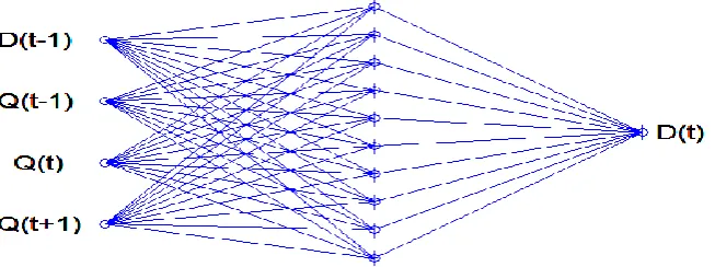
Structure of Bioreactor inverse neural network model at Lower input
During the identification and control tasks the NNSYSID (M. Nørgaard, 1996). and NNCTRL (K. J. Hunt, D. Sbarbaro, R. Zbikowski and P. J. Gawthrop, 1992) toolboxes for MATLAB are used.
6.1.1 Higher dilution rate (D =0.2278hr-1) 6.1.1.1 Servo problem:
The servo response has been studied by giving a step change in set point of productivity with direct inverse neural network and PI controller.
At lower dilution rate the servo problem has been analyzed by giving step change in set point of productivity from 3.0 to 3.1(+10%) and the corresponding responses are shown in fig.5.In this response the NNDIC+I reaches the set point at around 20 hrs without any offset whereas PI is reaching the set point at 60hrs.The corresponding manipulated variable in terms of dilution rate versus time behavior are shown in fig 6
Fig 7 shows the step change in the set point of productivity from 3.0 to 2.9.In this response the NNDIC+I reaches the set point at around 20 hrs without any offset whereas PI will reach the set point after 200 hrs.The corresponding manipulated variable in terms of dilution rate versus time behavior are shown in fig 8
6.1.1.2 Regulatory problem:
The regulatory response in productivity of direct inverse neural network controller and PI controller for dilution rate input of disturbance in feed substrate concentration have been studied and they are stated below:
The regulatory response in productivity of direct inverse neural network and conventional PI is shown in fig 9 for a step change in feed substrate concentration (Sf) from 20 to 22(+10%).This fig shows that the
response of the Direct inverse neural network controller is faster than that of the linear PI. Proposed neural network control has less deviation 2% whereas conventional PI controller has a larger deviation of about 35%. Direct inverse neural network controller has low settling time than the PI controller. The corresponding control actions for manipulated variable in terms of dilution rate versus time behavior are shown in fig 10
The regulatory response in productivity of direct inverse neural network and conventional PI are shown in fig 11 for a step change in feed substrate concentration (Sf) from 20 to 16(-20%).This fig shows that the
7. CONCLUSIONS
In the present work, the performance of conventional PI controller and Neural Network based controller is studied for the set point changes at higher input dilution rates. Based on the above studies the following conclusions are made.
At higher input dilution rate, response of PI controller for set point change from 3 to 3.1 g/l/h is stable with offset and for another set point change of 3 to 2.9 g/l/h is stable with offset response due to input multiplicities. Whereas proposed neural network based direct inverse controller is giving stable and faster responces.
REFERENCES
[1] Chidambaram,M and Reddy, G.P. (1995) Nonlinear control of systems with input multiplicities , Computers and Chemical Engineering, 19 pp249-252.
[2] Abonyi, J ,.Babuska, R. and Ayala Botto, M and Szeifert, F L. Nagy and Nagy (2002) Identification and control of nonlinear systems using fuzzy hammerstein models, Industrial & Engineering chemistry Research.39 pp4302-4314 .
[3] Dash, S.K. and Koppel, L.B.(1989) Sudden destabilization of controlled chemical Processes Chemical Engineering Communications, 84 , pp 129-157.
[4] Koppel,L.B. (1982) Input multiplicities in nonlinear multivariable control systems AIChE Journal.28 pp935 -945.
[5] Koppel, L.B.(1983) Input multiplicities in process control, Chemical Engineering Education, pp58-63, & 89-92.
[6] D.B.Anuradha, G.Prabhaker Reddy and , J.S.N.Murthy, “Direct Inverse Neural Network Control of A Continuous Stirred Tank Reactor”, Proc. IMECS, .2, Hong Kong,236-241,2009.
[7] M. A. Henson &.D.E. Seborg , “Nonlinear control strategies for continuous fermenter”, Chemical engineering Science, 47,821-835, 1982.
[8] K. Hornik, M. Stincombe, and H. White, "Universal approximation of an unknown mapping and its derivatives using multilayer feedforward networks", Neural Networks 3, 1990, pp.211-223.
[9] B. Kosko, Neural Networksand Fuzzy Systems: A Dynamic Systems approach to Machine Intelligence, prentice Hall, 1992.
[10] L. Fausett, Fundamentals of Neural Networks, New Jersey: Prentice-Hall, 1994.