An adjustable linear Halbach array

Author’s Accepted Manuscript

An adjustable linear Halbach array J.E. Hilton, S.M. McMurry

PII: S0304-8853(12)00100-X

DOI: doi:10.1016/j.jmmm.2012.02.014

Reference: MAGMA57359

To appear in: Journal of Magnetism and Magnetic Materials

Received date: 16 November 2011 Revised date: 25 January 2012

Cite this article as: J.E. Hilton and S.M. McMurry, An adjustable linear Halbach array,

Journal of Magnetism and Magnetic Materials,doi:10.1016/j.jmmm.2012.02.014

This is a PDF file of an unedited manuscript that has been accepted for publication. As a service to our customers we are providing this early version of the manuscript. The manuscript will undergo copyediting, typesetting, and review of the resulting galley proof before it is published in its final citable form. Please note that during the production process errors may be discovered which could affect the content, and all legal disclaimers that apply to the journal pertain.

An adjustable linear Halbach array

J. E. Hiltona,∗, S. M. McMurryb

a_{CSIRO Mathematics, Informatics and Statistics, Clayton South, VIC 3169, Australia} b_{School of Physics, Trinity College Dublin, Ireland}

Abstract

The linear Halbach array is a well known planar magnetic structure

ca-pable, in the idealized case, of generating a one-sided magnetic field. We

show that such a field can be created from an array of uniformly magnetized

rods, and rotating these rods in an alternating fashion can smoothly transfer

the resultant magnetic field through the plane of the device. We examine

an idealized model composed of infinite line dipoles and carry out

computa-tional simulations on a realizable device using a magnetic boundary element

method. Such an arrangement can be used for an efficient latching device,

or to produce a highly tunable field in the space above the device.

Keywords:

Magnetic field, Permanent magnet flux source, Halbach array, Simulation

1. Introduction

Applications requiring specifically tailored magnetic fields are widespread

in industry and research. The field sources for such applications come in a

diverse variety of shape and form, but can be approximately divided into

pow-∗_{Corresponding author}

ered and static categories. Powered sources use electromagnets, which require

an electric current to create the field. Static sources consist of arrangements

of permanently magnetized hard magnetic material, possibly augmented with

softer magnetic materials (Coey, 2002). Although far higher field strengths

can be reached with electromagnetic sources, static sources have the natural

advantage that they require no continuous input of energy.

The discovery in the 1970’s of magnetic materials with both high

coer-civity and remanence, such as SmCo and NdFeB compounds, spurred

devel-opment of static field sources as a viable alternative to powered field sources.

Of these an important subset are designs based on particular arrangement

of permanent magnetic sources known as a ‘Halbach array’, or a ‘flux sheet’.

The first such design was described by Mallinson (Mallinson, 1973) as a sheet

of magnetic material with an alternating magnetization pattern. This

partic-ular magnetization pattern gave the design the unique, and counter-intuitive,

ability to confine the magnetic field to only one side of the sheet.

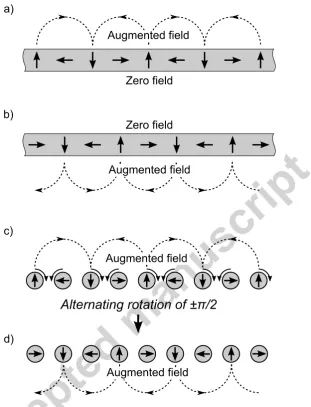
Continu-ous distributions of this pattern are shown in Figs. 1a and 1b, along with a

schematic representation of the resulting field. As the field is augmented on

one side and canceled on the other, the resultant field is effectively doubled

on the augmented side. Mallinson showed the field would be confined in this

manner if the components of magnetization were any Hilbert transform pair,

the simplest of which is m = sin(x)ˆi+ cos(x)ˆj, where m is the

magnetiza-tion vector and x the position along the sheet. A familiar example of such

a magnetization pattern is found in the polymer loaded ferrite material on

the back of fridge magnets. Such magnetic devices are now also widely used

Traveria, 1998), far from the ‘magnetic curiosity’ Mallinson described in his

original paper.

Rolling up such a flux sheet into a cylinder gives a field source known as

a ‘Halbach cylinder’, which was discovered independently by Klaus Halbach

during investigations into magnetic systems for particle accelerators

(Hal-bach, 1980). These remarkable designs can give a uniform, or multi-polar

field, confined entirely within the cylindrical bore of the design. Many

con-figurations and permutations of such cylinder designs are possible. Nesting

two Halbach cylinders allows a variable field within the bore of the device,

which can be precisely controlled by the relative angle between the two

cylin-ders (Ni Mhiochain, 1999). The magnetization distribution required for a

Halbach array can, remarkably, even be created by induced magnetization in

a highly permeable soft magnetic material (Peng, 2003). An idealized

infi-nite length Halbach cylinder produces an entirely uniform homogeneous field

within the bore of the cylinder. However, realizable designs suffer from ‘end

effects’ due to finite length, which reduces the field homogeneity within the

bore. Methods such as shimming and shaping the geometry (Hilton, 2007)

can correct this, significantly improving the uniformity of the field within

such finite length cylindrical designs.

Replacing the individual magnetic segments of a Halbach cylinder with

transversely magnetized rods allows the field within the bore of the design

to be controlled by the relative rotation of each rod. This design, called a

‘magnetic mangle’ was first suggested and investigated by Cugat (Cugat et

al., 1994). In this study we investigate a variation of this design in which an

the cylindrical axes, are arranged into a linear Halbach array. Rotating each

element of the array in the opposite direction to the neighboring elements

is shown to smoothly transfer the magnetic field from one side of the array

to the other. In a similar manner to how a linear Halbach array can be

considered an ‘opened’ Halbach cylinder, the structure investigated here can

be understood as an ‘opened’ magnetic mangle design. Although a wide

range of tunable field sources exist (Coey, 2002; Bjørk et al., 2010), including

designs based on movable Halbach arrays, this design appears to have been

overlooked. Arrangements of this design producing fields above and below

the plane of the rods are shown schematically in Figs. 1c and 1d, respectively.

In the following sections, we first investigate an idealized model of the

device using an array of infinite line dipoles. The resultant torques and

energy of each dipole are evaluated in order to asses the practicalities of any

such device. Then a finite size, realizable device is computationally modeled

using a magnetic boundary element method. We show that such a device

produces a strong, switchable magnetic field in the space above the device

and is not subject to excessive torques. Finally, we suggest a practical design

for such a device based on a simple gearing arrangement.

2. Modelling of the design

2.1. An array of magnetic line dipoles

The arrangement shown in Fig. 1c and 1d can be modeled, to a first

approximation, as a sequence of line dipoles. This basic model allows the

investigation of field and torque behavior on the dipoles as they are rotated

for a magnetic point dipole in Cartesian space, with unit vectorsˆi,ˆj, and kˆ

in the x, y and z directions, respectively. This is given by:

ψ(r) = m·r

4π|r|3 (1)

wherem is the point dipole moment. For a line dipole, confined to thex−y

plane and extending to ±∞ in the z direction, this becomes:

∫ _∞

−∞

m·r

4π|r|3dz =

λ·r

4π|r|2 (2)

where λ is the line dipole moment. The magnetic field of a line dipole is

significantly different to that of a point dipole. In polar co-ordinates the

field magnitude of a line dipole is independent of the polar angle to the

dipole, unlike a point dipole (Cugat et al., 1994). This effect is exploited in

arrangements such as this to provide the augmentation and cancellation of

the field on opposite sides of the plane of the dipoles. The scalar potential

from a collection of N such dipoles is given by:

ψ(r) = 1 4π

N

∑

a=1

λa·(r−ra)

|(r−ra)|2

(3)

where ra is the position of dipolea and the line dipole moment, in this case,

is given by:

λa(ϕ) =λ

(

sin[(−1)aϕ− aπ

2 ]ˆi+ cos[(−1)

a_ϕ− aπ

2 ]

ˆ_j) ₍₄₎

where ϕ is an overall rotation of the dipoles in the structure. It should be

noted that the rotational dependency onϕ for each dipole is opposite to that

arrangement where the dipoles are evenly spaced along thex axis, separated

by a distancel. This gives a final expression for the magnetic scalar potential

as:

ψ(r, ϕ) = 1 4π

N

∑

a=1

λa·(r−alˆi)

|(r−alˆi)|2 (5)

The torque on each dipole at rotation angle ϕ is an important measure

of the practicality of any device based on this design. The torque on dipole

b,τb, from the dipole array can be evaluated from Eq. (5) as:

τb(ϕ) =−

1

4πλb× ∇ N

∑

a=1,a̸=b

λa·(r−alˆi)

|(r−alˆi)|2 (6)

where the torque vector is aligned with the z axis. The energy of each

dipole allows the stability of the dipole at a particular rotation angle to be

investigated. The energy of a dipole in a field is given by U =−λ·H/µ0, so

the energy of a dipole b in the array is:

Ub(ϕ) = −

1

4πµ0λb · ∇ N

∑

a=1,a̸=b

λa·(r−alˆi)

|(r−alˆi)|2 (7)

2.2. Magnetized finite length segments

In order to investigate the practicalities of an actual magnetic device, the

arrangement was computationally modeled as a sequence of rods of hard

mag-netic material, uniformly magnetized perpendicular to the cylindrical axis.

The fields from these arrangements were calculated using a magnetic

bound-ary element method based on the magnetic charge model (Hilton, 2007). The

surface of each rod was decomposed into triangular sheets of magnetic charge,

as the summation of the fields from each of these sheets. The method has

been applied to a wide range of similar magnetic structures, and has been

carefully validated against existing analytical field solutions, as well as

exper-imental measurements of new magnetic designs (Hilton, 2007). The torque

on each magnet in the design can likewise be calculated from the torque

on each triangular charge sheet about the center of mass of each magnet.

The torque calculations have been verified by comparison to experimentally

measured torques (Ni Mhiochain, 1999) on complex magnetic structures.

3. Results

3.1. Field and torque of the dipole array

The expression for the array of infinite line dipoles was solved using the

computational package Mathematica. For convenience, the constant λ/4π

and the dipole spacing, l, were both set to unity. The resulting scalar

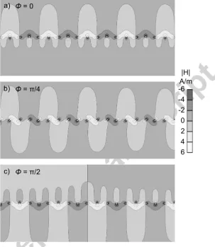
po-tential for a array of 65 line dipoles is shown in Fig. 2 at three rotation

angles. The field clearly reverses from above to below the plane of the line

dipoles as the dipoles are rotated alternately clockwise and anticlockwise as

ϕ is changed from 0 through to π/2 radians. The asymmetry in the scalar

potential is caused by end effects due to the finite number of dipoles in the

array. The scalar potential is symmetrical at ϕ = π/4 as the dipoles are

arranged in pairs orientated at ±π/4 radians to the vertical.

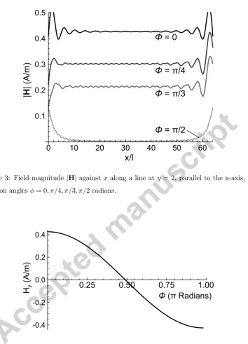
The field magnitude,|H|, along a line parallel to the x-axis at a position

y = 2 is shown in Fig. 3 for a range of ϕ. It should be noted that the

low values for |H|, in comparison to real-world magnetic structures, are due

discussion of the results, as we are concerned with only the form of the field

within this section. Oscillatory effects from the finite number of dipoles are

apparent at the start and end of the array, but the field magnitude over the

mid part is approximately uniform. Rotation of the array, surprisingly, does

not appear to affect the uniformity of the field magnitude, which smoothly

reduces to zero as each dipole in the array is alternately rotated through

ϕ = 0 → π/2 radians. At ϕ = π/2 radians the field magnitude at y = 2 is

reduced to zero.

The Hy field component at the mid point of the array, x = 32, at a

position y = 2 is shown in Fig. 4 for ϕ = 0 → π. The x-component of

the field, Hx ∼ 0 at this point for the entire range of ϕ. The y-component

smoothly varies as the cosine of the rotation angle, ϕ. The field is zero at

ϕ =π/2, as shown in Fig. 3, but reverses in the rangeπ/2→π

Torques on each dipole in the array were calculated from Eq. (6) and

are plotted against dipole position in Fig. 5. The effect of the finite number

of dipoles is again apparent at the start and end of the array. However, the

torque rapidly reaches a fixed value for dipoles only several steps from the

ends of the array. The torque on each dipole varies as the sine of the rotation

angle, reaching a maximum value at ϕ=π/4, and is approximately zero over

the bulk of the array at ϕ= 0, π/2.

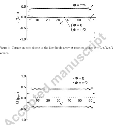
The energy of each dipole in the array was calculated from Eq. (7) and

is plotted against dipole position in Fig. 6 for ϕ = 0, π/2. At ϕ = π/4, all

dipoles have approximately zero energy. The energy minimum of a dipole at

ϕ = 0 orϕ=π/2 was found to occur at the energy maxima of its neighboring

showing that the dipoles are alternately at stable and unstable mechanical

equilibria at these orientations.

A series of line dipoles therefore shows the desired behavior, producing a

field which varies asHy ∼cos(ϕ). The largest torques are experienced by the

dipoles within the stray field regions at the ends of the array. The torques

within the bulk of the array are approximately zero for ϕ = 0 and ϕ =π/2.

However, each dipole at these orientations is either at an energy minimum or

maximum with respect to its neighboring dipoles, showing that mechanical

stabilization of the array is necessary for a practical device.

3.2. Field and torque of a magnetic rod arrangement

In the simple dipole model, end effects caused by the finite number of

dipoles were observed at the start and ends of the array. Practical

mag-netic designs also suffer from additional effects caused by the finite length of

the magnetic components in the design (Ni Mhiochain, 1999; Bjørk , 2011).

These can decrease both the effective magnetic field and the homogeneity

of the field over the working area of the device. To investigate these effects

in a realizable device, a practical sized magnetic design was modeled.

Six-teen transversely magnetized rods were used in the device, N = 16, with

a remnant magnetization of Br = 1.2T, typical of a standard grade of the

hard magnetic material NdFeB. The rods were chosen to be 10cmlong, with

diameter 1 cm, separated by an air gap of 2.5 mm between each rod. The

circular cross-section of each rod was discretized into a 20 sided regular

poly-gon, and the magnetic charge on each element was calculated from the dot

product of the element and the magnetization distribution within the rod,

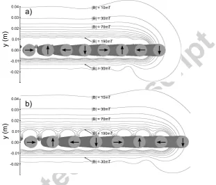
The magnetic flux density, |B|, from the arrangement is shown in Fig.

7, where only half the design is shown as the field is symmetrical about

the y axis. As expected, the field reverses as each rod is rotated alternately

throughϕ = 0→π/2. The magnitude of the field atϕ= 0, π/2 is reasonably

uniform and homogeneous within central part of the design, even for such an

arrangement consisting of only 16 rods.

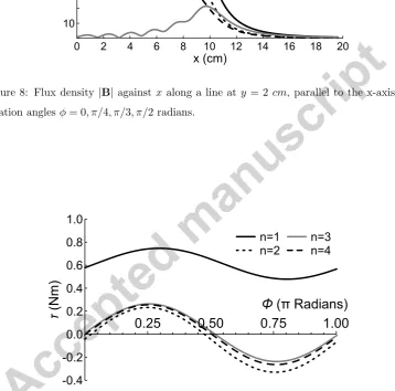
The flux density, |B|, along a line parallel to the x-axis at y = 2 cm

is shown in Fig. 8 for ϕ = 0, π/4, π/3, π/2. The end of the array is at

approximatelyx= 10cm. The field profile atϕ = 0 is similar to the array of

line dipoles, consisting of a constant field over the central part of the array

with an oscillatory stray field at the ends of the device. The field aty= 2cm

shows almost an ideal reduction from 75mT to zero as the magnetic segments

are rotated.

The torque on four rods in the design is shown in Fig. 9, where the torque

is evaluated about the center of mass of the rod. The four rods are labeled

in Fig. 7a as n = 1,2,3,4. The torque on each rod varies sinusoidally with

rotation angle ϕ, as found in the simplified line dipole model. Similarly, the

rods experiencing the maximum torques are located at the ends of the array.

The magnetic rod model therefore qualitatively agrees with the basic line

dipole model, showing the same field and torque variations with rotation

angle, ϕ.

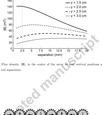
3.3. Variation of the geometry for the magnetic rod arrangement

The design can be readily optimized, as the field shows a non-linear

de-pendency on rod separation. The flux density, |B|, from the arrangement

ϕ = 0. Increasing the rod separation does not affect the field homogeneity

in the central region above the plane of the rods, and appears to slightly

increase the maximum magnetic field strength away from the plane of the

rods. A plot of the flux density against separation is shown in Fig. 11 at

x= 0 for several values of y. At large rod separations, |B| →0. The vertical

dashed line shows the 25 mm separation used in the preceding section. It

can be seen that the optimal spacing, giving the maximum field strength, at

any chosen vertical position above the rods varies with the vertical position.

4. Discussion

The magnetic field strength in the plane above a flux sheet is given, in the

idealized case, by |B|2 = Ke−ky (Mallinson, 1973). As the field varies with

the cosine of the rotation angle, the field in an arrangement of magnetized

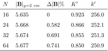
rods can therefore be approximated by |B|2 = K′e−k′ycos2(ϕ), where K′, k′

are constants depending on the magnetic remanence, rod separation and

other geometric factors. For the design discussed in the previous section,

with N = 16 and a rod separation of 25 mm, these constants were found

from data fitting to be K′ = 0.923, k′ = 256 for y > 1 cm. The field was

very close to the expected exponential form, with the natural logarithm of

the exponential fit having R2 = 0.9998. For designs with N rods, the field

was found to be relatively invariant for N > 16, with < 1% difference in

the measured field at y= 2 cm compared between designs with N = 16 and

N = 64. The field at y= 2 cm and the percentage difference in the field in

comparison to a design with N = 16 is given in Table 1 for a selection ofN,

N |B|y=2cm ∆|B|% K′ k′

16 5.635 0 0.923 256.0

24 5.668 0.582 0.866 252.1

32 5.674 0.691 0.855 251.3

64 5.677 0.741 0.850 250.9

Table 1: Flux density |B|at y = 2cm, ϕ = 0 for variousN, % difference in |B| from a

design withN = 16 and fitting parametersK′, k′.

Simulations show that such a design is easily realizable and will not be

subject to excessive torques during rotation on each of the rods. Mechanical

stabilization is required, however, as no global energy minima exist for the

system. Rods at energy minima, and stable mechanical equilibrium, have

neighbors at energy maxima at unstable equilibria. A very straightforward

solution exists, however, giving both mechanical stabilization as well as

al-lowing the ability to rotate rods alternately. This is simply to use an equal

gearing of each rod to the neighboring rod, as shown in Fig. 12. It can be

noted that a flux sheet can be discretized into more sections to give a

mag-netization pattern which varies more smoothly (Bjørk et al., 2010), but this

would require a far more complex gearing mechanism.

Such a design can be used for a range of practical applications. For

example, the latching strength of such a device varies with the cosine squared

of the rotation angleϕ. This can be shown by evaluating the Maxwell stress

tensor in the idealized case of a highly permeable soft magnetic material

parallel to the plane of the rods. The latching strength for each pole in the

device is then given by Flatch =N By2A/4µ0 (Furlani, 2001), where N is the

device, this gives Flatch ∼ Ncos2(ϕ)A/4µ0. For the design in the preceding

section with a rod separation of 25mm, this gives a maximum latch strength

on a soft magnetic plate aty= 2cmofFlatch∼180N, which smoothly varies

to zero as the rods are rotated.

5. Conclusion

A series of magnetized rods, arranged in the form of Mallinson’s flux sheet,

produces a field confined to one side of the plane of the rods. The field can

be transferred through the plane by alternating rotation of each rod. Such

an arrangement can be fabricated into a practical device by a simple gearing

arrangement, as shown schematically in Fig. 12. Such a device would have

a range of applications, such as a mechanical magnetic latching or a variable

field source. Two such parallel arrangements might be used as a variable

wiggler magnet for free electron laser and synchrotron devices. It is our hope

that this simple design, which appears to have been previously overlooked,

will be a useful addition to the family of tunable field source devices.

J. M. D. Coey, Permanent magnet applications, Journal of Magnetism and

Magnetic Materials 248 (2002), 441-456.

J. C. Mallinson, One-Sided Fluxes A Magnetic Curiosity? IEEE

Transac-tions on Magnetics, 9 (1973), 678-682.

J. Juanhuix, M. Traveria, Magnetic design and light characteristics of a

Wig-gler for the LLS, 6th European Particle Accelerator Conference,

K. Halbach, Design of permanent multipole magnets with oriented rare earth

cobalt material, Nuclear Instruments and Methods 169(1) (1980), 110.

T. R. Ni Mhiochain, D. Weaire, S. M. McMurry, J. M. D. Coey, Analysis of

torque in nested magnetic cylinders, Journal of Applied Physics, 86 (1999),

64126424

J. E. Hilton, S. M. McMurry, Halbach cylinders with improved field

homo-geneity and tailored gradient fields, IEEE Transactions on Magnetics 43(5)

(2007), 1898-1902.

Q. Peng, S. M. McMurry, J. M. D. Coey, Cylindrical permanent-magnet

structures using images in an iron shield, IEEE Transactions on Magnetics

39(4) (2003), 19831989.

O. Cugat, P. Hansson, J. D. M. Coey, Permanent Magnet Variable Flux

Sources, IEEE Transactions on Magnetics 30(6) (1994) 4602-4604.

R. Bjørk, C. R. H. Bahl, A. Smith, N. Pryds, Comparison of adjustable

permanent magnetic field sources, Journal of Magnetism and Magnetic

Materials 322 (2010) 36643671.

R. Bjørk, The ideal dimensions of a Halbach cylinder of finite length, Journal

of Applied Physics 109 (2011), 013915

E. P. Furlani, Permanent magnet and electromechanical devices: materials,

Figure 1: a) Continuous magnetization pattern generating a one-sided field above the plane

of the magnet. b) Continuous magnetization pattern generating a one-sided field below

the plane of the magnet. c) Discretization of the continuous distribution generating a field

above the plane of the magnet. d) Discretization of the continuous distribution generating

a field below the plane of the magnet. Alternating clockwise and anti-clockwise rotation

Figure 2: Contours of magnetic scalar potential for a element array of line dipoles, with

Figure 3: Field magnitude |H| againstxalong a line aty = 2, parallel to the x-axis, at

rotation angles ϕ= 0, π/4, π/3, π/2 radians.

Figure 4: Field componentHy aty = 2 in center of array as a function of rotation angle

Figure 5: Torque on each dipole in the line dipole array at rotation anglesϕ= 0, π/4, π/2

radians.

Figure 6: Energy of each dipole in the line dipole array at rotation angles ϕ= 0, π/4, π/2

Figure 7: Flux density, |B| for array of magnetized rods, with rotations a) ϕ = 0, b)

Figure 8: Flux density |B| againstxalong a line at y = 2 cm, parallel to the x-axis, at

rotation angles ϕ= 0, π/4, π/3, π/2 radians.

Figure 10: Flux density, |B| for array of magnetized rods, with ϕ = 0 and spacing a)

Figure 11: Flux density, |B|, in the center of the array at four vertical positions as a

function of rod separation.

Figure 12: A straightforward implementation of the device using an equal mechanical

We model an adjustable ‘one sided’ flux sheet made up of a series of dipolar magnetic field sources.

We show that magnetic field can be switched from one side of sheet to other by an swap rotation of each of magnetic sources.

Investigations show that such an arrangement is practical and can easily be fabricated.