Kauffman

(1)

Forestry & Natural-Resource Sciences Last Correction: Mar. 27, 2016

AUTOMATED ESTIMATION OF FOREST STAND AGE USING

VEGETATION CHANGE TRACKER AND MACHINE LEARNING

Jobriath S. Kauffman, Stephen P. Prisley

Center for Natural Resources Assessment & Decision Support, Virginia Polytechnic Institute & State University, USA

Abstract.The ability to automatically delineate forest stands and determine their age is useful for natural

resources professionals. Two common approaches to estimating forest area and age-class distributions are inventory-based methods, such as Forest Inventory and Analysis (FIA), and remote sensing based methods. Vegetation Change Tracker (VCT) is an algorithm that uses time series stacks of Landsat images to identify forest disturbances. However, additional computation is required to identify type of disturbance. This paper evaluates the usefulness of machine learning tools, such as support vector machine (SVM), for reclassifying VCT disturbances as stand-clearing disturbances or partial disturbances. Overall accuracy for a 2010 VCT disturbance map of the entire state of Virginia was determined to be 87 percent. 100 percent of 2010 Virginia clearcut harvests recorded in a reference dataset were classified as disturbances by VCT. Neighboring disturbed pixels, as classified by VCT, were clumped together and reclassified as stand-clearing disturbances or partial disturbances using SVM and variables for average disturbance magnitude and shape and size metrics of the clumped pixels, with an overall accuracy rate of 86 percent. The users and producers accuracy rates for stand-clearing disturbances were 88 percent and 95 percent respectively. In addition, an algorithm was developed in R for determining years since last stand-clearing disturbance for each pixel in a time series stack of reclassified VCT disturbance maps from 1984 to 2011. Neighboring pixels of the same age, in number of years since last stand-clearing disturbance, were clumped together and correspond, in general, to clearcut harvest boundaries.

Keywords: forest disturbance, harvest type, forest age, harvest delineation, automated, machine learning.

1 Introduction

The fact that there is value in mapping forest stands is unquestioned. Distributions of forest by stand age and type at various spatial scales provide valuable infor-mation for optimizing forest production and sustainabil-ity. Both field measured forest inventories and remotely sensed data have been used to estimate forest area and age. Each of these methods has its strengths and limi-tations. Precise field measured inventory estimates from sample plots are possible over large areas but are costly for fine scale estimates across a large area due to the large number of sample plots required. Remotely sensed data can be obtained just as easily for a specific point as it can for an entire image. Automated processing of these large amounts of data is an obstruction that is be-coming easier to overcome. While cost effective methods for yearly, statewide, border-to-border mapping of forest by age and major species group have been elusive they are nonetheless obtainable.

The U.S. Forest Service Forest Inventory and Analysis program (FIA) comprises the most comprehensive field measurement of forest inventory today. The sampling process utilizes a hexagonal grid system placed over the forty-eight contiguous states. Each of the hexagons cov-ers approximately six thousand acres. A forest inventory plot is randomly located within each hexagon. Trees are measured on four subplots within each plot, totaling approximately 1/6 of an acre (Bechtold and Patterson 2005).

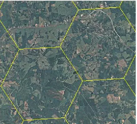
Virginia contains approximately 4700 sampling hexagons. This large sample size allows for accurate estimates over large areas comprising the entire state or multiple counties. However, Figure 1 demonstrates that there can be a great amount of variation in forest distri-bution over a six thousand acre hexagon that cannot be represented on a small scale by one FIA plot. This high-lights the value of smaller scale representation of timber products and biomass at the stand or pixel level.

Copyright c2016 Publisher of theMathematical and Computational Forestry & Natural-Resource Sciences

(2)

Kauffman et al. (2016)/Math. Comput. For. Nat.-Res. Sci. Vol. 8, Issue 1, pp. 4–13/http://mcfns.com 5

Figure 1: Representation of variation in forest distribu-tion over 6000 acre hexagons in central Virginia.

Timber product volume and biomass estimates at small scales are difficult to obtain but increasingly valu-able for sustainvalu-able forest management. Maps of forest by major species groups are common, including nation-wide land cover mapping such as the 30 meter pixel scale National Land Cover Database (NLCD) land cover map (Homer et al. 2015). Age estimates, in combination with forest type, from remote sensing data at the stand or pixel level can make a major contribution towards fur-ther refining volume estimates at this small scale.

A simple way to calculate “age” of a forest is to mea-sure the number of years since the last clearcut. Algo-rithms using time series stacks of Landsat data, such as Vegetation Change Tracker (VCT), have proven to be reliable for detecting forest disturbances (Huang et al. 2010). After other known dark objects such as water and dark soils have been masked from Landsat images dating back to 1984 (Landsat 4), VCT uses forest training pix-els identified from the forest peak in histograms of top of atmosphere reflectance in the near infrared and two short-wave infrared spectral bands (Huang et al. 2008, Huang et al. 2010). The means and standard deviations of these training pixels in the red and shortwave infrared bands are used to calculate an integrated forest z-score (IFZ) for each pixel in the image (Huang et al. 2010).

In time series of yearly height of season IFZ values, forested pixels will remain persistently below a threshold IFZ value, while non-forested pixels will remain above the threshold or fluctuate above and below it (Huang et al. 2010). Thus, a sudden increase in a pixel’s otherwise persistently low IFZ score indicates the timing of a for-est disturbance within the time series. In this way, the VCT algorithm described by Huang et al. (2010) can be

used to generate VCT products such as yearly distur-bance maps at the 30 meter pixel level. The magnitude of these disturbances can also be calculated by finding the difference between a pixel’s average IFZ score (or other index) and its IFZ score for the disturbance year. Normalized difference vegetation index (NDVI) and nor-malized burn ratio index (NBRI), and IFZ4 are also in-corporated in the VCT algorithm and used to calculate similar measures of disturbance magnitude (Huang et al. 2010). NDVI measures photosynthetic capacity us-ing the red and near-infrared bands. The calculation for NBRI is similar to NDVI but uses the near-infrared band and short-wave infrared band (band 7). Changes in NBRI can be used to measure burn severity. IFZ4 is cal-culated similarly to IFZ but uses only the near-infrared band. Maps of disturbance magnitudes of disturbed pix-els measured each of these ways are in production for the contiguous United States.

Within secondary succession forests, especially those in which frequent harvest and regeneration occurs, groups of neighboring 30 meter pixels representing forest of the same age were most likely harvested together, or cleared by some other mechanism, at some point in the past. Clumping these neighboring pixels of the same age together can be used as a method for creating objects that conform to past harvest boundaries.

The Virginia Department of Forestry began keep-ing records of all harvests in Virginia in 2009 in order to facilitate inspections of best management practices (BMPs). The GPS point location of the first logging deck the BMP inspector comes to on the date of in-spection is collected along with other harvest attributes. Typically, there are five or six thousand harvests per year in Virginia. Delineating these harvests with a GPS during inspection or by post-harvest photo interpreta-tion is costly and time consuming. Therefore, efforts to automate this process and extend the records back to 1984, the first available year of VCT disturbance maps, are worthwhile.

(3)

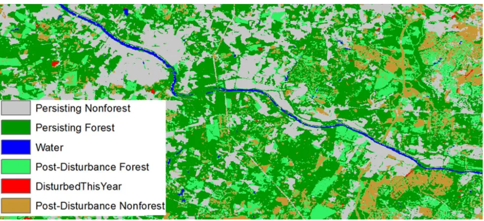
Figure 2: Portion of 2010 Virginia VCT map.

This research demonstrates procedures for using yearly VCT disturbance maps to create clumps of neigh-boring pixels that were disturbed collectively. These clumps can then be spatially linked to recent harvest records, and metrics related to shape, size, and aver-age disturbance magnitude of each clump can be used to train machine learning tools used for classifying dis-turbances as either stand-clearing or partial. Through-out this paper the term “enhanced VCT” will be used when referring to VCT disturbance maps that have been reclassified to include only stand-clearing disturbances. Raster stacks of stand-clearing disturbance maps can be used to subsequently create an “age” map by calculating the number of years since the last stand-clearing distur-bance. The process for creating a map of this type for Virginia will be described in the next section. VCT data products are anticipated to be available nationally, cre-ating opportunities to repeat these methods anywhere in the contiguous United States, especially in areas domi-nated by harvest disturbances.

2 Methods

2.1 2010 VCT disturbance map validation VCT disturbance maps and disturbance magnitude maps cre-ated from the VCT algorithm were obtained for all of Virginia. An accuracy assessment of the 2010 VCT dis-turbance map for Virginia was performed using before and after aerial photography, 2008 National Agriculture Imagery Program (NAIP) and 2012 NAIP respectively. Figure 2 depicts a portion of the 2010 VCT disturbance map. VCT yearly disturbance maps are classified into

six groups: persisting non-forest, non-forest after a dis-turbance, persisting forest, forest after a disdis-turbance, forest disturbed in the current year, and water. 100 sample points within each class were randomly chosen. For simplicity the two non-forest groups (200 points to-tal), and the two forest groups (200 points total) were combined together. This assessment can be used to val-idate the accuracy of using the map to identify each of these classes, including forest and forest disturbances.

2.2 Evaluating the ability to detect clearcuts In conjunction with the 2010 VCT disturbance map accu-racy assessment the ability of VCT to detect clearcut harvest was evaluated. VCT mapped all sample points that were clearcuts as disturbances. In order to add weight to this assessment the Virginia harvest records were used to look for possible errors outside of the sam-ple used for validation in which VCT classified a clear-cut harvest as something other than a disturbance. All harvest locations that did not intersect a VCT distur-bance were inspected using the before and after aerial photography in order to find out if there was perhaps a stand-clearing disturbance that VCT missed. If VCT is doing reasonably well at detecting stand-clearing dis-turbances, the next step would be to reclassify all VCT disturbances as stand-clearing or not.

(4)

to allow for more cloud free pixels. The latest scene used for Virginia in 2009 was taken on September 14th, while the earliest scene taken for Virginia in 2010 was on June 3rd. Therefore, point locations of Virginia tim-ber harvest data records from the Virginia Department of Forestry for inspections between these dates were in-tersected with the 2010 VCT disturbance maps cover-ing Virginia. This encompasses all of the land area in Virginia within Landsat path/row scenes 14/34, 14/35, 15/33, 15/34, 15/35, 16/33, 16/34, 16/35, 17/33, 17/34, 17/35, 18/34, 18/35, 19/34, and 19/35.

Cells classified as disturbances within each VCT dis-turbance map were evaluated for adjacency to neighbor-ing disturbed cells with the Queen’s case of 8 directions (right, left, above, below, or diagonal) using the ‘clump’ function in the R ‘raster’ package (Hijmans 2015). In this manner, connected groups of neighboring disturbed pixels were assumed to be the result of the same forest disturbance. Therefore, they were clumped together and given a common identity. Since VCT detects both stand-clearing disturbances and partial disturbances, the abil-ity to calculate stand “age” must be facilitated by re-classifying VCT disturbances as stand-clearing or not. Classification of VCT disturbances by type using ma-chine learning tools, including SVM, is appropriate and has proven to be effective (Zhao et al. 2015).

Average VCT disturbance magnitudes as measured by IFZ, NDVI, NBRI, and IFZ4 were obtained for each dis-turbance clump. In addition, various shape and size metrics were calculated for each clump using the ‘Patch-Stat’ function in the ‘SDMtools’ R package (VanDer-Wal et al. 2014). Clearcut harvests tend to have higher disturbance magnitudes, larger areas, and less complex shapes as they conform to more linear parcel boundaries. There were 1170 VCT disturbance clumps from 2010 that intersected with one of the harvest site point lo-cations in the date range specified above. Half of the disturbance clumps were used for training and half for validation of three machine learning tools used to reclas-sify VCT disturbance clumps as stand-clearing or par-tial disturbances. k nearest neighbor (kNN; Meyer et al. 2015), support vector machine (SVM; Venables and Ripley 2002) , and the ‘rpart’ (Therneau et al. 2015) R package classification algorithms were trained using a somewhat arbitrary selection of variables, including dis-turbance magnitudes measured three ways (IFZ, NDVI, and NBRI), area, and fractal dimension index of the training clumps. Fractal dimension index is a measure of shape complexity. The kNN algorithm classifies a point in the feature space according to the majority class of a predefined number of nearest neighbors. SVM is also a supervised classification algorithm that maximizes the separation between two classes with a hyperplane. The ‘rpart’ package is an implementation of the

Classifica-tion and Regression Trees (CART) algorithm, following Breiman et al., 1984 in most details. CART and rpart recursively split the feature space by finding the value of a variable that separates the training sample data into classes that minimize incorrect classification. In an ef-fort to maximize automation of the reclassification pro-cess, no further effort was made to calibrate the models or select the most advantageous features for improving accuracy. For the kNN algorithm, k=9 was arbitrar-ily chosen for the number of nearest neighbors. Kernel methods for producing non-linear classifiers are possible with SVM, but the default ‘linear’ kernel was used for simplicity. Each of the three trained models was used to classify each member of the validation set as a stand-clearing disturbance or a partial disturbance, and the results were compared to the actual harvest data.

The trained machine learning classification tools were used to reclassify each clump in each disturbance map as a stand-clearing disturbance or not based on the ma-jority class of the three models. This process was au-tomated and repeated for the 15 Landsat scenes for the entire study area, each year for the 28 years from 1984 to 2011, using R and its “raster” package (R Core Team 2015, Hijmans 2015). The resulting maps of stand-clearing disturbances are what has been defined above as enhanced VCT disturbance maps.

2.4 Calculating age R was also used to create a time series stack of the enhanced VCT maps in order to calcu-late the “age” of each pixel by determining the number of years since the last stand-clearing disturbance. Neigh-boring pixels of the same “age” using the Queen’s case of 8 directions were clumped together and the “Elim-inate” filter function in Erdas Imagine (Leica Geosys-tems 2013) was used to clean edges and eliminate small clumps less than five pixels. Thus, clumps smaller than one acre were removed, and those pixels were back-filled with information from the surrounding clumps.

3 Results

(5)

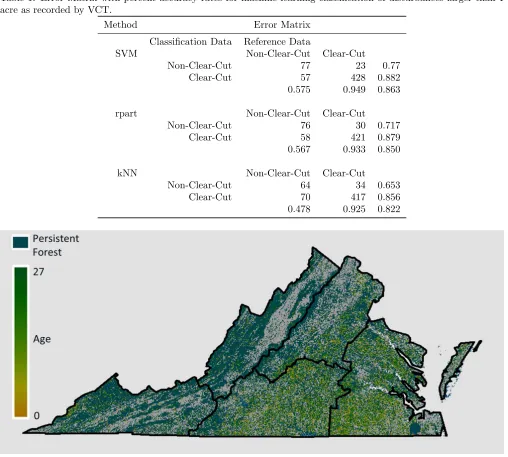
Table 1: Error Matrix with percent accuracy rates for machine learning classification of disturbances larger than 1 acre as recorded by VCT.

Method Error Matrix Classification Data Reference Data

SVM Non-Clear-Cut Clear-Cut

Non-Clear-Cut 77 23 0.77 Clear-Cut 57 428 0.882 0.575 0.949 0.863

rpart Non-Clear-Cut Clear-Cut

kNN Non-Clear-Cut Clear-Cut

Figure 3: Virginia VCT “age” map enhanced by reclassifying disturbed pixels as stand-clearing or not.

the harvest site and are sometimes outside of the har-vest site altogether, so it is not expected that all harhar-vest point locations will be within the actual boundaries of the harvest.

The greatest overall reclassification accuracy rate was achieved with SVM at 86 percent (Table 1). SVM cor-rectly classified 95 percent of clearcuts but misclassified 42.5 percent of partial harvests. The results for kNN and rpart were comparable.

An enhanced VCT “age” map for all of Virginia was created (Figure 3). This map shows age as the number

(6)

regener-Kauffman et al. (2016)/Math. Comput. For. Nat.-Res. Sci. Vol. 8, Issue 1, pp. 4–13/http://mcfns.com 9

ated to the point that VCT can discern it is forest, with IFZ values remaining above the forest threshold.

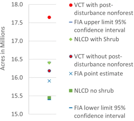
The enhanced VCT estimate of forest acres after re-moving post-disturbance non-forest pixels is within the 95 percent confidence bounds of FIA forest acre esti-mates using the 2011 population evaluation group, and is less than 2 percent higher than the FIA point es-timate (Miles 2016). It is also comparable to forest area estimates using the 2011 NLCD land cover map (Homer et al. 2015). The NLCD “shrub/scrub” class includes true shrubs and young trees less than 5 meters tall. Much of what is classified as shrub in Virginia is actually early successional forest or trees stunted from environmental conditions. Therefore two NLCD totals are shown in Figure 4. The first includes the decidu-ous forest, evergreen forest, mixed forest, and woody wetlands classes without shrub. The second also in-cludes the “shrub/scrub” class. The NLCD estimates are very close to the lower and upper 95 percent confi-dence bounds of the FIA estimate, respectively.

Figure 4: Estimates of forested acres in Virginia.

Figure 5 compares forest area estimates for the en-hanced VCT with FIA in Virginia by age class (Miles 2016). These estimates generally coincide, but special note should be made where enhanced VCT estimates fall outside the confidence bounds of FIA. In addition to low area estimates when excluding the pixels that no longer look like forest in the 0-5, 6-10, and 21-25 year age classes, and the high estimates when includ-ing these pixels in the 0-5 and 11-15 year age classes, the enhanced VCT also overestimates forest acres when compared with FIA in the over 25 age group, even when post-disturbance non-forest pixels are excluded. The

es-Figure 5: Forested acres in Virginia by age class, up to age 25.

timate without post-disturbance non-forest pixels in this age group is 12.5 million and rises to 12.7 million when these pixels are included. Possible reasons for these dif-ferences will be discussed in the next section.

Figure 6 shows the tendency of clumps of neighbor-ing reclassified VCT disturbances of the same “age” to conform to actual harvest boundaries. These clumps also frequently conform to parcel boundaries (Figure 7). Figure 8 shows how the resulting enhanced VCT gets rid of isolated pixels and provides a more realistic determi-nation of stand “age” by reclassifying disturbed pixels in a 2010 thinning as a partial disturbance, giving the accurate number of years since the most recent stand-clearing disturbance.

4 Discussion

This study demonstrates both the value of compre-hensive harvest records for use in training and validating machine learning models as well as the ability to success-fully classify disturbance clumps by harvest method uti-lizing shape metrics in an automated manner. It is the intent that similar automated methods will be used to reclassify VCT disturbances and create forest age maps and harvest boundaries in other areas of interest.

(7)

accu-Figure 6: Depiction of ability of enhanced VCT to conform to harvest boundaries. Top: post-harvest NAIP aerial photography with photo-interpreted harvest boundaries; Bottom: Same image overlaid with semi-transparent en-hanced VCT ”age” raster.

racy rates. Also, algorithm parameters were not tuned to maximum accuracy. Some strategies that would not hinder automation while improving accuracy can and will be implemented. Four disturbance magnitudes and various shape and size metrics were calculated for each disturbance clump. One simple method for selecting from these variables would be to exclude one variable from each pair of highly correlated variables while

(8)

Figure 7: Depiction of conformance of enhanced VCT stand-clearing disturbances to parcel boundaries.

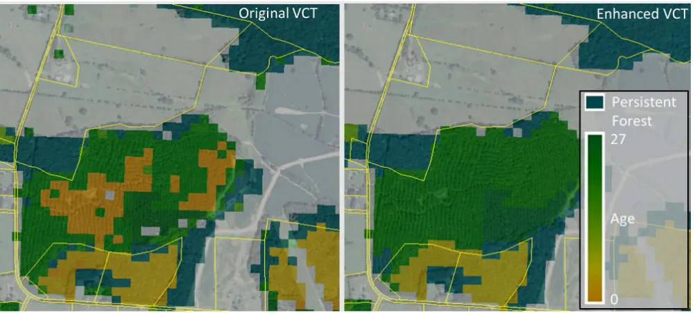
Figure 8: The enhanced VCT map reduces salt and pepper effects and more accurately depicts stand age by reclas-sifying disturbances such as this 2010 thinning as a partial disturbance before calculating years since most recent stand-clearing disturbance.

It is possible that the method used to sample clumps of disturbed pixels is biased towards clearcuts over par-tial harvests. Parpar-tial harvests often appear as multiple disjoint clumps in the same parcel rather than one solid clump like most clearcuts. Thus, it seems that there is a smaller chance that the logging deck of a partial harvest will intersect a VCT disturbance clump. The actual pro-portion of disturbances that are stand-clearing is likely

(9)

sample indicates that if VCT detects all stand-clearing disturbances and an equal area of partial disturbances, the overall map accuracy rate could be as low as 76 per-cent. On the other hand, by including parcel data, it is likely that the number of disjoint clumps in a cel could be a useful feature to help to distinguish par-tial harvests and improve accuracy. Parpar-tial harvests are more likely to appear as several disjoint clumps within the same parcel, while clearcuts most often appear as one contiguous clump.

In addition, the model used to classify harvest dis-turbances as stand-clearing or not is also used for other disturbances detected by VCT. This would indicate that the sample is biased towards harvest disturbances. The concern here seems to be minimal because harvests are the overwhelming disturbance type by area in Virginia. Other disturbances are likely to be so small that they will not affect stand age. Nonetheless, opportunities ex-ist to reclassify VCT dex-isturbances using auxiliary GIS data. These include conformance with parcel bound-aries, shape metrics of disturbance clumps, LiDAR for-est structure metrics, and variables such as distance to road and slope. Harvests are unlikely to occur in areas that are far from a road or with steep slope.

It should be noted that because a percentage of the pixels with an associated age have converted to non-forest and the number of years until regeneration begins depends on forest type and management intensity, there is room for improvement in the enhanced VCT “age” map. An analysis of the percentage of pixels that were classified as cleared according to the methods of this pa-per and return to forest according to VCT in one-year increments after disturbance is underway. Percentages can be calculated by forest type and/or ecoregion in or-der to shed light on differences in time to detect regen-eration using VCT.

When considering the area estimates in Figure 4 and Figure 5 it is important to note that there are differ-ences in how forest is defined by VCT, FIA, and NLCD (Huang et al. 2010, Bechtold and Patterson 2005, Homer et al. 2015). VCT uses a threshold cutoff of an inte-grated measure of number of standard deviations above the mean a pixel’s brightness in the red and two short-wave infrared Landsat bands is compared to the average of a forest sample. FIA imposes area, width, stocking, and use restrictions which are not accounted for with VCT. The figures for NLCD do not include developed open space which can include vegetation planted in de-veloped areas for recreation, erosion control, or aesthetic purposes. In addition the shrub/scrub class can include forest areas where there are young trees in an early suc-cessional stage that are less than 5 meters tall. However, this class and the woody wetlands class can also include true shrubs, of which there is very little in Virginia. It is

reasonable to believe that the total forest acres estimate for the enhanced VCT exceeds FIA because there are less restrictions on what it defines as forest.

Furthermore, higher estimates for enhanced VCT over FIA are not consistent across age classes when excluding VCT classified post-disturbance non-forest. This reveals a time lag after a disturbance before VCT can detect a return to forest. It is conceivable that the reclassified enhanced VCT stand-clearing disturbance maps and the enhanced VCT age map derived from them can be in-telligently combined with information from NLCD or a similar land cover map to arrive at a more accurate age map. For instance, a disproportionately high number of pixels that are classified as forest by VCT but grassland by NLCD are in the 0-5 age group. Thus, VCT forest pixels estimated to be older according to enhanced VCT and are also classified as grassland according to NLCD are less likely to be forest with the correct age estimate. Perhaps some of these pixels were incorrectly classified by VCT as forested and some are actually young forest with incorrect older age estimates.

5 Conclusion

While the enhanced VCT product is a good proxy for “age” and generally conforms to harvest boundaries, some work remains. Despite the overwhelming presence of secondary succession forest in Virginia due to clearcut harvesting practices in the south, a majority of the forest in Virginia has not been disturbed since 1984. Therefore its age cannot be precisely determined, and large clumps of undisturbed forest cannot be broken up into stand-sized pieces using reclassified VCT disturbances. These stand-sized pieces would be a good basis for modeling future change. It may be possible to use variables such as LiDAR height and structure metrics along with other remotely sensed and auxiliary GIS data to create these stand-sized units.

Additional work needs to be done to generate iden-tities for unique harvests rather than unique clusters. Partially forested parcels may include disjoint clumps of harvested pixels even if the harvest was a clearcut. Therefore parcel data should be combined with VCT data to identify disjoint clearcut harvest clumps that are most likely part of the same clearcut harvest. This could be important for modeling efforts in which only harvests that meet a minimum area threshold are con-sidered. For instance, small harvests may be excluded when modeling commercial wood supply. Further pro-cessing should be done to combine adjacent clumps that differ by one VCT year because a single harvest spanned consecutive VCT years.

(10)

as stand-clearing disturbances or not based on average disturbance magnitude, shape, and size results in a good proxy for “age” and objects that conform to harvest boundaries. The net result is an historical record of har-vest boundaries that can also be used to predict when and where future harvests will occur. A decades long historical record begins to shed light on the impact of variables such as policy change, social and cultural val-ues, and ownership demographics on harvesting prac-tices, although their overall impact may not be known for many more decades. Estimates of biomass or timber volume across time provide valuable data for procure-ment foresters, landscape ecologists, climate scientists, water resource experts, and many others.

Acknowledgments

We are very grateful to Chengquan Huang for gener-ously sharing the data that this work is based on. Spe-cial thanks to the anonymous reviewers whose dedica-tion and insightful feedback significantly improved our manuscript. Thanks also to the Center for Natural Re-sources Assessment and Decision Support and its part-ners for their support of this project.

References

Bechtold, W.A., and P.L. Patterson. 2005. The en-hanced Forest Inventory and Analysis Program– national sampling design and estimation procedures. USDA For. Serv. Gen. Tech. Rep. SRS-GTR-80. 88 p. Breiman, L., J.H. Friedman, R.A. Olshen, and C.J. Stone. 1984. Classification and regression trees. Wadsworth. 368 p.

Hijmans, R.J. 2015. raster: Geographic data analy-sis and modeling. R package version 2.4-18. Last ac-cessed online on Jan. 19, 2016, at: http://CRAN.R-project.org/package=raster.

Homer, C.G., Dewitz, J.A., Yang, L., Jin, S., Daniel-son, P., Xian, G., Coulston, J., Herold, N.D., Wick-ham, J.D., and Megown, K. 2015. Completion of the 2011 National Land Cover Database for the conter-minous United States–representing a decade of land cover change information. Photogrammetric Engineer-ing and Remote SensEngineer-ing. 81(5):345–354.

Huang, C., L.S. Davis, and J.R.G. Townshend. 2002. An assessment of support vector machines for land cover classification. International Journal of Remote Sensing. 23(4):725–749.

Huang, C., K. Song, S. Kim, J.R.G. Townsend, P. Davis, P. Masek, and S.N. Goward. 2008. Use of a dark

ob-ject concept and support vector machines to automate forest cover change analysis. Remote Sensing of Envi-ronment. 112:970–985.

Huang, C., S.N. Goward, J.G. Masek, N. Thomas, Z. Zhu, and J.E. Vogelman. 2010. An automated ap-proach for reconstructing recent forest disturbance history using dense Landsat time series stacks. Re-mote Sensing of Environment. 114:183–198.

Leica Geosystems. 2013. ERDAS Imagine version 2014. Atlanta, Georgia.

Meyer, D., E. Dimitriadou, K. Hornik, A. Weingessel, and F. Leisch. 2015. Misc functions of the Department of Statistics, Probability Theory Group (formerly: E1071), TU Wien. R package version 1.6-7. Last ac-cessed online on Jan. 19, 2016, at: http://CRAN.R-project.org/package=e1071.

Miles, P.D. 2016. Forest Inventory EVALIDa-tor web-application version 1.6.0.03. USDA For. Serv., Northern Research Station, St. Paul, MN. Last accessed online on Jan. 26, 2016, at: http://apps.fs.fed.us/Evalidator/evalidator.jsp.

Pal, M., and P. Mather. 2005. Support vector machines for classification in remote sensing. International Jour-nal of Remote Sensing. 26:1007–1011.

R Core Team. 2015. A language and environment for statistical computing. R Foundation for Statistical Computing, Vienna, Austria. Last accessed online on Jan. 19, 2016, at: https://www.R-project.org/.

Therneau, T., B. Atkinson, and B. Ripley. 2015. rpart: Recursive partitioning and regression trees. R package version 4.1-10. Last accessed online on Jan. 19, 2016, at: http://CRAN.R-project.org/package=rpart.

VanDerWal, J., L. Falconi, S. Januchowski, L. Shoo and C. Storlie. 2014. SDMTools: Species Distri-bution Modelling Tools: Tools for processing data associated with species distribution modelling ex-ercises. R package version 1.1-221. Last accessed online on Jan. 19, 2016, at: http://CRAN.R-project.org/package=SDMTools.

Venables, W.N., and B.D. Ripley. 2002. Modern applied statistics with S, 4th ed. Springer, New York. 498 p.