44
Data Processing Methods for Deep Level Transients
Measurement
Pham Quoc Trieu, Hoang Nam Nhat
*Faculty of Physics, VNU University of Science, 334 Nguyen Trai, Thanh Xuan, Hanoi, Vietnam
Received 17 December 2018
Revised 20 December 2018; Accepted 22 December 2018
Abstract: The year 2019 marks 45 years in the development of Deep Level Transient Spectroscopy (DLTS) - the signal processing method for determination of overlapping deep levels in semiconductors. From its introduction in 1974 by David Lang (D.V. Lang, J. Appl. Phys. 45, 1974, p.3023) to this date the DLTS method has undergone many changes and modifications: some were purely theoretical speculations, some were to include new experimental arrangements and techniques. This paper provides a short review on DLTS data processing techniques, focusing on the main three approaches widely used today. We also summarize the contribution of our group in the Faculty of Physics, VNU University of Science.
Keywords: DLTS, Boxcar, Arhenius plot, Fourier, Laplace, Deep levels, Traps.
1. Introduction
Deep traps play important role in physics of materials but the characterization of those deep traps faced many difficulties until an introduction of Deep Levels Transient Spectroscopy (DLTS) by D. Lang in 1974 [1]. The method was new by its time, but appeared rather too late as the semiconductor industry seems to out-run its maximum output and role in the history. Later in 2001, the first DLTS equipment from Bio-RAD was installed in Center for Materials Science, Faculty of Physics, VNU-Hanoi University of Science. This method allows the detection of overlapping deep centers by simple recording of capacitance transients according to time t in varying temperature T. Its success at the early time was unambiguous but later it shows a limiting accuracy and low overall resolution, together with high sensitivity to random noise. Since then, many improvements have been proposed but the method still struggles against low resolution until today. However, from the view point of data processing technique, this method is extremely interesting and appears useful in many other aspects of applied sciences, as it offers a practical solution to a very old problem of how to separate the
________
Corresponding author. Tel.: 84-913097735. Email: [email protected]
overlapping exponential functions, recall that the capacitance dependence on time as C(t)Ceent,
where t is time, C a scaling constant and enso called an emission factor.
By utilizing a double boxcar circuit to record the transient C(t), the author of [1] can obtain a signal of form S(T)=C(t1)C(t2). This function may be flat with no peak structure, but it can show
maxima at certain temperatures if the deep traps occur. If one scans S(T) over several T then one can construct a plot of ln(e/T2) vs. 1000/T to determine the trap parameters (Fig. 1).
T e m p e r a t u r e
S
(T
)
s e t t in g 1 s e t t in g 2
T im e
C(
t)
a
t
v
a
ri
o
u
s
T
s e t t in g 2 s e t t in g 1
Fig. 1. The different settings of gate windows S(T)=C(t1)C(t2) at fixed T (right part) and the
maxima of S(T) at two fixed rate windows according to varying T (left part) [15].
Up to date, among the data processing techniques that have been reported [2-19], there are two that attracted application: the Fourier and the Laplace technique. Both do not have the rate windows, they measure rather one value of C(T) at one time (the sampling includes either 512 or 1024 measured points), and require only one temperature scan. Although the resolution and scan time were sufficiently improved, the accuracy and separability are still low, while strongly affected by noise (either thermal or random white noise). Also, as they do not involve any rate windows then the exact emission factors (obtained at the maximal gains) can not be calculated in advance. The correspondences between the peaks and the deep centers appear in the two methods somehow subtle and arbitrary. It is worth to mention that in the Lang's original approach the setting of rate window means the selection of emission factor for which the rate window reacts mostly. We briefly discuss the Lang's signal form in the section below.
2. Lang's signal form
A discussion of Lang approach in the language of the signal forms appeared in [15]. A common task of all spectroscopic methods is to find the analytic functions which transform the measured data (in our case, the transients CT(t) recorded at specific T) into the specific functions fn(T), whose peak
structures (according to T in our case) can be analyzed. The fn(T) functions are usually referred to as
the spectroscopic functions and the corresponding methods the spectroscopic ones. For C(t) the functions need to satisfy a condition of linearity, that is, the Arhenius plots [ln(e/T2) vs. 1000/T]
obtained from the measured C(t) are linear. Here we call the fn(T) functions the signal forms. There is
not known any spectroscopic signal forms other than the Lang's, Fourier and Laplace forms until the intervention of [15]. In general, the capacitance transient can be given as:
C t C
Cieeit0
)
where C0 is C(t=), C=Ci = C(t=0)C0 and i denotes the number of present deep traps.
Now, let us denote normalized values of capacitance as Cn(t)=(C(t)C0)/C, and put t1=td,
t2=t+d, for d is a half width of a gate window, then the Lang's signal can be given in the form:
( ) ( ) ( / )[ ]
)
(T Cn t d Cn t d Ci C e ei(t d) e ei(t d) S
(2)
If the traps are far from each other in the energy scale, then we can differentiate S(T) according to some emission factor ei, while leaving the other ej zeroed, to determine the signal maximal gain.
Taking from [1] the maximum gain can be given using the variables t and d as follows:
emax = ln[(t+d)/(td)]/2d (3)
It is evident from eq. (3) that by providing t and d the emission factor emax is determined.
3. Fourier DLTS
The pre-historical idea how to obtain an optimal set of emission constants {i =1/ei , c0 and ci}
from eq.(1) is to involve a least square technique. But this was not successful due to occurrence of false extremes. A correction of Lang's original technique comes from Weiss and Kassing in 1988, and a method is called the Fourier DLTS [4]. The Fourier DLTS is an integral method since it does not measure directly C(t) but a correlation integral R(t) with some periodical filter f(t) with period Tw:
w T
w
dt T t C t f T T t R
0
, 1
) ,
( (4)
This integral passes through maximum at certain T when m(T) is equal to values preset by filter
f(t). This signal sufficiently improves the accuracy, resolution and stability but among the disadvantages belongs the fact that it loses many important information containing in C(t, T), so the radical improvement is limited. We know from the definition of the Fourier series that, a differentiable continuous real and periodical function c(t) having period Tw (i.e. c(t) = c(t+nTw) with all n=0,1,2...)
can be decomposed into a Fourier series:
1
0 cos 2 sin 2
2 ) (
n w
n w n
T nt b
T nt a
a t
c
(5)an , bn are the Fourier coefficients:
w
T
w w
n nt dt
T t c T a
0
) 2 cos( ) (
2
(6)
w
T
w w
n nt dt
T t c T b
0
) 2 sin( ) (
2
(7)
In case the c(t) is a complex function, the complex coefficients cn are defined as:
w wT
nt T i
w
n
c
t
e
dt
T
c
0
2
)
(
1
(8)
cn
anibn
21
(9)
For the discrete Fourier analysis, c(t) has only N particular values c(tk), k=0,1,..., N in a period Tw,
and the integral (8) becomes:
Nk
N k n i
k
n
c
t
e
F
02
)
(
(10)And there is an empirical dependence between the coefficients Fn and their complex counterparts cn:
F
n
Nc
nD (11) where D is an empirical real constant. The equation (11) is of great importance for the Weiss and Kassing method because it allows to calculate cn on the basis of N measurements c(tk).Now look at the integral output
w T
w
dt
t
C
t
f
T
t
R
0
)
(
)
(
1
)
(
of the signal C(t) and we see that:- the integral output R(t) plays a role of the Fourier coefficients cn ;
- the filter f(t) has the form
2
w
i nt
T
e
with period Tw.
With this intuition, the involving of Fourier series in DLTS becomes clear. The basic procedure is as follows:
a) at some specific T, measure N values of C(tk) for various times tk = kk1. The
period of C(t) will be Tw = Nt. Now find R(tk) for each C(tk).
b) suppose that c(t) follows the exponential decay and c(t) is a real function; let the filter f(t) be
nt T i
w
e
2
we can calculate the Fourier coefficient an , bn and cn.
c) now suppose C(tk) = c(tk) and we calculate Fn and cn according to (11) and find the experimental
values of anand bn
d) by comparison of theoretical and experimental values anand bn we can find at a given T and a
trap concentration NT.
e) now by repeating the steps (a), (c) and (d) one can find all possible (T). At the final, one can build the Arhenius plots and determine the activation energy ET.
The Fourier method requires only one temperature scan, the time can be determined directly from the experimental coefficients an and bn measured at each T. In the Lang's approach, one must first
fix the rate-windows then scan T and in the Fourier DLTS, one first fix T then scan all rate-windows (512 or 1024 measurements) to find . Suppose we have one trap center emitted according to the exponential law:
0
)
(
t t
Ae
B
t
C
(12)The Fourier coefficients are determined as:
e
e
B
T
A
a
w T t
w
2
1
2
00
22 2
/
2
/
1
/
1
1
2
0 w T t w nT
n
e
e
T
A
a
w
(14)
22 2 / 2 / 1 / 2 1 2 0 w w T t w n T n T n e e T A b w
(15)
So we have:
w w T t n w T n T n e e b T A w / 2 / 2 / 1 1 2 2 2 2 1 0
(16)By dividing an and bn for each other, we have several ways to calculate :
n k k n w k n a n a k a a T a
a 2 2
2 ) , (
(17)
n k k n w k n kb n nb k nb kb T b
b 2 2
2 ) , (
(18) n n w n n a b n T b a
2 ) ,( (19)
In the Fourier DLTS the four values (a1, a2), (b1, b2), (a1, b1) and (a2, b2) are mostly used and
among them the (a1, b1) is usually most correct. With n=1 we have a simple relation between a1, a2,
b1 and b2. This relation can be used to check whether or not the measured coefficients (a1, a2, b1,
b2)MEAS do follow the exponential law of emission:
2 1 2 2 1 1 b a a b (20)
If (20) does not hold so the emission is probably caused by overlapping centers.
4. The algebraic structure of reference levels
It seems unobserved from the first time of DLTS that the right part of equation (3) is almost equal to 1/t numerically. One can easily prove that ln[(t+d)/(td)]/2d really converges to 1/t when the half width of the rate windows d0 by using the Euler number definition n n e
n
(1 1/ )
lim . By giving
that ln[(t+d)/(td)]/2d ~ 1/t, the emax corresponds to Cn(t)=e1 (Fig. 2). For this reason Cn=e1 is called
a reference level of S(T). Now consider a moving of gate from t to t'=at, the emission factor changes as ei(t') = ei(at) = 1/at = (1/a)ei(t). Thus, the transient associated with gate t' will have at time t an
emission factor equal to that of the transient associated with gate t at time t/a:
a n n a t t e t t e t C a t C e
0 .0 0 .2 0 .4 0 .6 0 .8 1 .0 1 .2
0 5 0 1 0 0 1 5 0 2 0 0 2 5 0 3 0 0
t[m s ]
Cn
(t
)
a
t
v
a
ri
o
u
s
T
C =1/e
G ate t
em a x
Fig. 2. A reference level: a rate window [td, t+d] shows a maximum according to T when the Cn(t) decreases through a point Cn(t)~1/e=0.368 [15].
So a modified Lang's signal, to be called a signal of order a, can be given as:
S(T)[a] =C
n(td)1/aCn(t+d)1/a (21)
which produces a maximal output along a reference level Cn=ea. The S(T)[a] forms a class of
signals, which is referred to as a Lang's signal class. Evidently, emax{S(T)[a]}= a ln[(t+d)/(td)]/2d =
aemax{S(T)[1]} = a/t. This signal class associates each point X [y=ea, x=t] with one horizontal line
(y=ea) and one vertical line (x=t). It is obvious that:
ei(a,t)= aei(1,t)= ei(1,t/a) (22)
ei(a,t)n= anei(1,t)n=anei(1,tn)= ei(an,tn)=ei(1,(t/a)n)
This tells us about the equivalence of all techniques involving the double boxcars. We can check ref. [15] to reveal the following relations:
[ei(a,t)+ei(b,t)] = ei(a,t)+ei(b,t)= aei(1,t)+bei(1,t) = a+b)ei(1,t) = ei((a+b),t) (23)
[ei(a,tn) ei(b,tm)] = ei(a,tn) ei(b,tm)=
= aei(1,t)nbei(1,t)m=(ab)ei(1,t)n+m= ei{(ab),tn+m)} (24)
5. The signal classes and forms
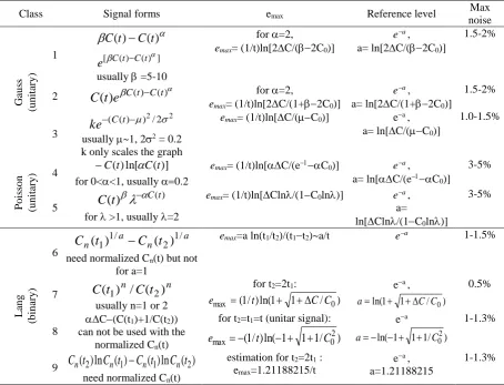
We summarize two classes of signal forms, a Gaussian and a Poisson class (to the later S(T)[a]
reduces as a special case), which possess the algebraic structure as that of S(T)[a]. These classes are
summarized in Table 1, where the last column shows the maximal pseudo-random noise level (in % of maximal signal) that does not disturb emax values more than 5%. As mentioned in ref.[15], among the
unitary signal forms, the Poisson signals (derived from the Poisson distribution) are most accurate. The Gaussian forms are also good but are also more sensitive to noise. Both classes are of ea reference level with emax=a/t. Fig. 3 compares some of them with a classic Lang's form (middle quality
0 1 2 3 4 5 6 7
0 1 0 0 2 0 0 3 0 0 4 0 0 5 0 0
T e m p e r a t u r e [ K]
S ig n a l fo r m s [ a .u .]
G a u s s ia n 1
L a n g 's 9
Po is s o n 4 L a n g 's 1
Fig. 3. Comparison of some selected signal forms to a classical Lang's S(T) form for a sample with one trap E=0.44eV.
Table 1. The finit element signal classes: signal forms, their emax and reference levels [15]
Class Signal forms emax Reference level
Max noise Gau ss (u n itar y )
1 [ () () ]
) ( ) (
t C t C e t C t C usually =5-10
for =2,
emax= (1/t)ln[2C/(2C0)]
ea,
a= ln[2C/(2C0)]
1.5-2%
2
C
(
t
)
e
C(t)C(t) for =2,emax= (1/t)ln[2C/(1+2C0)]
ea,
a= ln[2C/(1+2C0)]
1.5-2%
3
2 2/2
) ) (
(
C t
ke
usually ~1, 2 = 0.2 k only scales the graph
emax= (1/t)ln[C/(C0)] ea, a= ln[C/(C0)]
1.0-1.5% Po is so n (u n itar y
) 4 C(t)ln[C(t)] for 0<<1, usually 0.2
emax= (1/t)ln[C/(eC0)] ea, a= ln[C/(eC0)]
3-5%
5
) (
)
(t C t
C
for >1, usually =2
emax= (1/t)ln[Cln/(1C0ln)] ea, a=
ln[Cln/(1C0ln)]
3-5% L an g (b in ar y ) 6 a n a
n t C t
C (1)1/ ( 2)1/
need normalized Cn(t) but not for a=1
emax=a ln(t1/t2)/(t1t2)~a/t ea 1-1.5%
7 n n t C t
C(1) / ( 2)
usually n=1 or 2
for t2=2t1:
) / 1 1 ln( ) / 1 ( 0
max t C C
e
ea, ) / 1 1
ln( C C0 a
0.5%
8
C(C(t1)+1/C(t2)) can not be used with the
normalized Cn(t)
for t2=t1=t (unitar signal):
) / 1 1 1 ln( ) / 1
( 02
max t C
e
ea ) / 1 1 1
ln( C02 a
1-1.3%
9
C
n(
t
2)
ln
C
n(
t
1)
C
n(
t
1)
ln
C
n(
t
2)
need normalized Cn(t)estimation for t2=2t1 : emax=1.21188215/t
ea, a=1.21188215
6. Averaging functions
We now discuss the averaging functions, as the increase of accuracy and separability of all transient-processing methods depends a lot on filtering noises. At recent time, the resolutions of all applicable DLTS methods are quite limited. This is why they cannot be utilized in other important areas of experimental physics, such as in high energy physics, astronomy and related areas, although high demands are seen for accurate analysis of transients.
6.1. Time averaging functions: the correlation of signals at fixed T
The correlation integrals at a fixed variable are equivalent to averaging according to this variable [17]. There are several simple correlation functions that can be easily derived. Let be a period width, the cross-correlation of Cn(t) and 1/Cn(t) becomes:
n n n e t e t e e dt e e R
2 / 2 / ) ( 1 )( Ln(R( ))en
1
(for all T) (25)It is interesting that the autocorrelation of L(t) is pretty simple:
12 1 ) ( 2 2 / 2 / n n n n e dt e t e t eR
(26)
And the autocorrelation of L(t)/t can also be obtained straighforward:
2 2 / 2 / 1 ) ( n n n n e dt t e t e t t e
R
(27)One may also check that a cross-correlation between L(t)-1/t and 1/L(t)-1/t is always 1:
( ) 1 1
2 / 2 /
dt e t e t t t e R n n n (28)These results are very interesting and useful as they show how the emission factors can be calculated as the averaging functions.
6.2. Temperature averaging functions: the correlation of signals at fixed time
To filter the thermal noise, let us write
T -2 / e T t
-e
(T ) n C
, L(T)-1/t
T2e/T and put TLnT Ln
T L
Ln[ ( ) 1/t]
2
/
M(T) .
A cross-correlation between M(T) and 1/M(T) is:
2 1 2 1 2 ) ( 2 2 1 ) ( 1 ) ( T T T T T T TT e dT
T T T dT e T e T T R
(29)Now substitute x=1/T, x1=1/T1, x2=1/T2, x=x2-x1 and denote A=(1/x)Ln(x1/x2),
) ( 2 1
1 2
R
B A
Ln (30)
The is a temperature shift in the unit of 1/T. The correlation function directly determines the activation energy of deep level.
6.3. Temperature shift operator Cn(Tp) = Tp[Cn(T)]
Let Cn(T) be a normalized capacitance signal at certain gate t . Denote L(T) = Ln[Cn(T)] and
M(T) = Ln[-Ln(Cn(T))]. According to temperature, the shift operator
T
p moves Cn(T) ontoCn(Tp), for p is a real positive constant: Cn(Tp) =
T
p[Cn(T)].By dividing Cn(Tp) by Cn(T) we can arrive at [17]:
)] 1 1 ( [ 2
[
p e T p
(T)
C
(T)]
C
(Tp)
C
nT
p n n (31)Similarly, we can obtain
)] 1 1 ( [ 2
[
T p
e p
L(T) L(T)]
L(Tp) Tp and
) 1 1 (
2
[
p T p
Ln
M(T) M(T)]
M(Tp) Tp . Let denote =E/k we have:
L(T)] L(T)
[ 1
2
p T
p Ln p p T
(32)
So an arbitrary shift from L(T) to L(Tp)determines a energy constant significant within this temperature segment. Ref. [17] shows that not only but also can be detected via the shift operators.
7. Vibrated boxcar technique
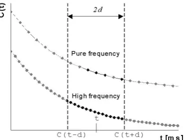
In this section we describe a measurement system which monitors the capacitance transient signals C(t) at the preset T by a variable multiplicator - a vibrating boxcar. The main idea bases on a single boxcar which instead of being fixed at certain position, vibrates with some preset frequency.
If we now imagine the decreasing of the capacitance signal over time t through a region [td, t+d] when the gate - set up before at a central position t vibrates with amplitude d, than the result C from a multiplicator circus should lie in the range [C(t-d), C(t+d)] (see Fig. 4). Giving t, d and by measuring C, the emission factor e(T) can be deduced directly without a repeated scan of temperature.
Fig. 4. The occurrence of the transients when the gate vibrates with various frequencies. When the frequency was set large enough compared to a proper relaxation time then the whole band of transient is recorded. Otherwise at lower vibrating frequency only some segments of transient falls
within a gate vibration interval.
enough in comparison with a proper relaxation time of the transient, then the recorded values should fill a whole band [C(t-d), C(t+d)]. If F is comparable to a relaxation time then only several occurrences should be recorded and if F is too small then no point could be recorded. We now consider only a case where the whole band [C(t-d), C(t+d)] is fulfilled with the transients. In general the emission factor depends on temperature according to a relation:
0 2exp( )
kT E T
e
e (33)
where e0 is a pre-factor depending on level concentration and capture cross section, E is the
activation energy and k is Boltzmann constant. In term of e the capacitance transient C(t) reads:
C
(
t
)
C
0
C
exp(
et
)
(34) A standard signal is defined as:S(T)C(td)C(td)C[exp(e(td))exp(e(td))] (35)
And by scaling S(T) on C and removing exp(et) out of the brackets we have ]
) exp(
1 ) )[exp( exp(
) (
ed ed
et C
T S
.
By denoting ]
) exp(
1 ) [exp( ],
) ( [ ) (
ed ed
Ln C
T S Ln T
s
we have finally:
s(T)et
(36) Providing that d is preset the is always a constant, the s(T) signal can be obtained by setting:s(T) = Cmax Cmin (37)
requires only one temperature scan and among advantages it does not require a temperature step to be set too fine as for other methods. In general, it needs only 5 temperatures to be maintained, so the measuring time is greatly shortened. The temperature step can be set as large as the whole temperature band divided by 5. The sensitivity of this method is strongly correlated with vibrating frequency. The method is resistible to the occurrence of random noise, since the statement (37) is already averaged so is not very much affected by the random noise.
9. Conclusion
Although many algorithms have been involved in the industrial manufacturing of DLTS equipments such as in the Fourier BIO-RAD DL5000 systems, the development is still going on to improve further the resolution of the method. The newest studies promise more sensibility and faster measurement process while providing more complex outputs and enhancement of ability of the method.
Acknowledgements
This research is funded by Vietnam National Foundation for Science and Technology Development (NAFOSTED) under grant number 103.02-2017.18. Apart of this work has been done in the Laboratory for Low Dimensional Materials and Application, Faculty of Engineering Physics and Nanotechnology, VNU-University of Engineering and Technology. We also thank the Center for Materials Science (CMS), VNU-Hanoi University of Science for providing access to the equipment.
References
[1] D.V. Lang, J. Appl. Phys. 45, (1974) p.3023.
[2] de Prony, Baron Gaspard Riche (1795). Essai éxperimental et analytique: sur les lois de la dilatabilité de fluides élastique et sur celles de la force expansive de la vapeur de l'alkool, à différentes températures. Journal de l'École Polytechnique, Vol.1, cahier 22, 24-76.
[3] Osborne, M.R. and Smyth, G.K. (1991). A modified Prony algorithm for fitting functions defined by difference equations. SIAM Journal of Scientific and Statistical Computing, 12, 362-382.
[4] S. Weiss & R. Kassing, Solid State Electronics, Vol. 31, 12 (1988) p. 1733
[5] L. Dobaczewski, P. Kaczor, I.D. Hawkins, A.R.Peaker, Mat.Sci.and Tech. 11 (1994) p. 194-198. [6] H. N. Nhat & P. Q. Trieu, VNU-J. of Sci. T-XVIII, No. 4 (2002) 32-39.
[7] C. Hurtes, M. Boulou, A. Mitonneau, D. Bois. Appl. Phys. Lett. 32 (1978) p.821-823.
[8] J. Morimoto, M. Fudamoto, K. Tahira, T. Kida, S. Kato, T. Miyakawa, Jap. J. Appl. Phys. 26 (10) (1987) p.1634 [9] M. Pawlowski, Rev. Sci. Instrum., 70 (1999) p. 3425-3428.
[10] M. Okuyama, H. Takakura, Y. Hamakawa, Solid-State Elect., 26 (1983) p.689-694. [11] F.R.Shapiro, S.D.Senturia, D.Adler, J.Apply.Phys., 55 (1984) p.3453.
[12] Z. Su, J.W.Farmer, J. Apply. Phys., 68(1990), p.4068.
[13] I. Thurzo, D. Pogany, K. Gmucova, Solid-State Elect., 35 (1992) p.1737-1743. [14] K. Ikeda, H. Takaoka, Jap.J.Appl.Phys.,21(1982) p.462-466.
[15] H. N. Nhat, P. Q. Trieu, VNU-J. of Sci. T-XVIII, No. IV (2002) 28-36. [16] M. Schwartz et al., Comm. Systems & Techniques, McGraw-Hill 1966, p.63 [17] H. N. Nhat, P. Q. Trieu, VNU-J. of Sci. T-XX, No. I (2004) 14-18
![Fig. 1. The different settings of gate windows S(T)=C(t1)C(t2) at fixed T (right part) and the maxima of S(T) at two fixed rate windows according to varying T (left part) [15]](https://thumb-us.123doks.com/thumbv2/123dok_us/1243230.1629407/2.595.165.438.213.323/different-settings-windows-maxima-fixed-windows-according-varying.webp)
![Fig. 2. A reference level: a rate window [td, t+d] shows a maximum according to T when the Cn(t) decreases through a point Cn(t)~1/e=0.368 [15]](https://thumb-us.123doks.com/thumbv2/123dok_us/1243230.1629407/6.595.182.398.120.287/reference-level-window-shows-maximum-according-decreases-point.webp)