An Inverse Problem Approach for Content Popularity
Estimation
Felipe Olmos
Orange Labs and CMAP, École Polytechnique∗
[email protected]
Bruno Kauffmann
Orange Labs[email protected]
ABSTRACT
The Internet increasingly focuses on content, as exempli-fied by the now popular Information Centric Networking paradigm. This means, in particular, that estimating con-tent popularities becomes essential to manage and distribute content pieces efficiently. In this paper, we show how to properly estimate content popularities from a traffic trace.
Specifically, we consider the problem of the popularity in-ference in order to tune content-level performance models, e.g. caching models. In this context, special care must be taken due to the fact that an observer measures only the flow of requests, which differs from the model parameters, though both quantities are related by the model assump-tions. Current studies, however, ignore this difference and use the observed data as model parameters. In this paper, we highlight the inverse problem that consists in determining parameters so that the flow of requests is properly predicted by the model. We then show how such an inverse prob-lem can be solved using Maximum Likelihood Estimation. Based on two large traces from the Orange network and two synthetic datasets, we eventually quantify the importance of this inversion step for the performance evaluation accuracy.
Categories and Subject Descriptors
C.2 [Computer-Communication Networks]: General
Keywords
Popularity Distribution, Mixture Model, Maximum Likeli-hood Estimation, Performance models, Caching
1.
INTRODUCTION
“Content is king”, says nowadays a popular Internet meme. This advent of ubiquitous content is reflected on the Inter-net, both by the importance of Content Distribution Net-works (CDNs) and transparent caching for coping with an
∗Centre de Math´ematiques Appliqu´ees, ´Ecole
Polytech-nique, CNRS, Universit´e Paris-Saclay.
.
ever-increasing traffic demand, and by the emergence of the Information Centric Networking (ICN) paradigm. Under-standing content and, in particular, its popularity is now es-sential to improve the Internet and its applications. Content-level performance models are therefore a key tool in the anal-ysis, design and dimensioning of networks.
Sparse models are particularly useful, since they capture the salient features of the system while remaining simple enough for analysis, depending only on a few parameters. These parameters have a large impact on the model out-put; yet one cannot observe them directly in measurements. Carrying a sensible analysis using the chosen model there-fore requires solving the inverse problem to find the best model parameters of the system from the measurements.
Due to the rise of content, the number of available doc-uments and their popularity distribution are now key pa-rameters for traffic models. They have attracted significant attention from the community in the context of user gener-ated content [3, 9], HTTP traffic [10, 13], and peer-to-peer networks [4, 19]. However, the measurement methods used in these works are not suited for parameterizing a perfor-mance model. In fact, they fail to take into account that the request count for a given document in a given observa-tion period, within the framework of a stochastic model, is not a fixed value, but a random variable. In particular, they ignore the fact that, in traffic traces, objects with no request are not observed, being thus azero-censored sample.
Our main objective in this paper is to provide a sound methodology for popularity estimation, with the aim of cor-rectly fitting performance models. This requires to take into account the stochastic relation between the model parame-ters and the request counts that are observed in a given dataset. To this aim, we follow [4] in constructing Maxi-mum Likelihood (ML) estimates. We illustrate the afore-mentioned issues and methodologies in the case of Poisson based traffic models in the context of caching performance. Nonetheless, the essential paradigm that we propose is ap-plicable to other traffic models and contexts. Note that the choice of relevantmodels is outside the scope of this paper.
The rest of this paper is organized as follows. We first re-view the literature in Section 2, and describe in Section 3 the datasets we use. We then explicitly identify and formulate in Section 4 the inverse problem that consists in correctly cal-ibrating performance models from trace measurements. To our knowledge, such a formulation has not been provided in previous studies. In Section 5, we propose a ML estimation method for this inverse problem. Section 6 provides a nu-merical evaluation of our approach. We discuss our results
VALUETOOLS 2015, December 14-16, Berlin, Germany Copyright © 2016 ICST
and possible extensions in Section 7.
2.
RELATED WORK
The works we here review falls into two broad categories: content popularity estimation from traffic measurements and statistical methods for mixtures models.
Due to the fact that popularity distributions usually ex-hibit a power law behavior, a common method to estimate them is to fit its rank-frequency distribution in double loga-rithmic scale. This approach has been recently criticized by Clauset et al. [4]. The main issue is that the rank-frequency plot is not a reliable statistic since, for example, it can ex-hibit power-law behavior even if the ground-truth does not. Despite these problems, the use of the latter method is still pervasive in performance evaluation [8, 11] and traffic char-acterization studies [12, 13, 2]. Authors try to improve these methods by means of various adjustments. In [13], for exam-ple, authors separate in three parts the rank-frequency plot adjusting different curves in each piece and in [12], authors adjust “stretched exponential” curves instead of power-laws. The latter adjustments indeed solve some of the fitting issues. In previous studies [11, 17], we have noted another issue in the context of performance models, which arises from the fact that it is permitted to objects to have zero re-quest. In consequence, from the point of view of the network operator, objects with no request are not observed in traces. In the statistical jargon, this is calledzero-censored and not taking this fact into account leads one to underestimate the catalog size, which has an impact on the conclusions drawn from the fitted model (see Section 6).
In the present work, we address the previous issues by using ML estimates. This method allows us to seamlessly handle the zero-censored case and it is proposed by Clauset et al. [4] as a robust method to fit heavy tailed data, which is a common property in popularity distributions. Maxi-mum likelihood methods have already been in use for flow size estimation [16] and call center modeling [18]. The latter work uses an approach similar to ours, but it is limited to a specific parametric model for non-censored data. More im-portantly, our work highlights the fact that the assumptions of the performance model must be taken into account for a proper popularity estimation.
The statistical basis of our methods is the estimation of mixed discrete distributions, a subject that has been exten-sively studied in the literature. The non-parametric case has been addressed from two points of view: the first one searches the mixing density in the space generated by La-guerre polynomials with an exponential cut-off; the estima-tor is then obtained by a projection on the latter space [20, 5]. It, however, converges slowly with the sample size un-less the density belongs to the aforementioned space. We therefore base our methodology on the second point of view, which assumes the mixing distribution to be a sum of Dirac masses. The estimation methods are then similar to an Expectation-Maximization scheme (EM) [15]. As regards the parametric case, EM schemes for finding the parameters of the mixing distribution are provided for many families in [14]. In both parametric and non-parametric cases, the estimation algorithms do not handle the case of censored data, and thus we simply use an all-purpose nonlinear opti-mization solver to obtain our results.
3.
DATASETS
We base our analysis on two real-traffic datasets, called #yt and #vod respectively. Dataset #yt comes from the YouTube traffic delivered for three months in 2013 by the Orange Network in Tunisia, while#vodcomes from the Video-on-Demand Orange service in France for 3.5 years. The traffic consists in 46 000 000 (resp. 3 400 000) requests to 6 300 000 (resp. 120 000) videos in the#yt(resp. #vod) set. More details on the collection and processing of these two datasets can be found in [17].
We also use two synthetic datasets, called#prtand#delta. This allows us to highlight in a more clear way some of our findings and, more importantly, to validate the results with controlled experiments when the ground-truth is not avail-able. The set#prt(resp.#delta) is generated by first draw-ing 10 000 000 (resp. 100 000) random samples with distri-bution Pareto (1.6,0.1) (resp. Dirac delta at 4.0) represent-ing the popularity (see section 5.1 for a model description). The number of requests for each document is then drawn according to the Poisson distribution with mean equal to the document popularity. After discarding the documents with zero request, this results into 2 600 000 (resp. 400 000) requests to 1 900 000 (resp. 98 000) documents.
4.
PROBLEM DEFINITION
In the following, we are given a stochastic object-level model predicting some performance indicator. The pre-dicted performance explicitly depends on a few parameters which characterize each object (e.g., document popularities, lifespans, sizes). It also strongly depends, however, on some implicit assumptions about the traffic or request process.
An example of such a situation is the evaluation of the hit ratio of a Least Recently Used (LRU) Cache, which is typically performed using the Independent Reference Model (IRM). In this context, users request documents among a catalog ofKdocuments. These requests are intercepted by a cache server, which can store and serve only an evolving subset of the catalog. The IRM assumes that the sequence of requests for document 1≤k≤Kis a Poisson process with intensityλk, where λk is proportional to the popularity of
document k; all such processes are mutually independent and their superposition build up the total request process. In this model, the numberNkof requests for documentkin a
time windowW is an independent Poisson random variable
P(λkW) of mean λkW. Up to a time normalization, we
assume in the following thatW = 1.
Figure 1 illustrates those two stages, both for an arbitrary performance model and the IRM case. The first stage con-sists in mapping the model parameters to a request flow (or a request flow distribution). The second step of the model computes the performance indicator, based on this request flow. In order to keep this paper concise, we now limit our-selves to the IRM model (see Section 7.1 for extensions).
Assume now that an observer has access to a sample of the actual request flow, e.g., a trace dataset or server logs. In the case of IRM, a sufficient statistics of the request process is the request countsn1, n2, . . . , nK0 for all observed
docu-ment, whereK0is the number of observed documents in the
Model parameters
Request Flow
Performance Indicator
K, λ1, λ2, . . . , λK
e
K, n1, n2, . . . , nKe
C7→H(C)
Figure 1: Schematic view of a performance model (left); example in the IRM case (right)
model using these parameters represents the data at best. A simple solution, henceforth called thenaive method, is to estimate the popularity of a document by its request count and the catalog size by the number of observed objects, that is: ˆKnv=K
0 and ˆλnvk =nk, for 1≤k≤Kˆnv.
We identify two problems at this stage. First, since the trace is zero-censored, with high probability the observed number of documentsK0 is strictly smaller than the
cata-log size K. Second, each document popularity λk is
esti-mated by a single samplenkof the random countNk. This
last limitation is well illustrated in the case of the#delta dataset. By definition, the ground-truth (real) popularities are λk = 4. In the dataset, however, the counts of
docu-ment requests are Poisson random variables of mean 4, hence ˆ
λnv
k =P(4) and the naive estimation “dilutes” the mass of
popularities over the set of positive integers. In Figure 2, we
0 0.2 0.4 0.6 0.8
0 0.2 0.4 0.6 0.8 1
H
it
Ra
ti
o
Relative Cache Size
GT Fit Naive
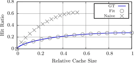
Figure 2: Hit ratio of a cache fed by #prt trace: ground-truth (GT) and prediction by the naive estimation. The cache size is normalized with respect to that of the GT.
show the impact of these limitations for the hit ratio estima-tion, based on the#prttrace. The first curve is our ground-truth. It is obtained via simulation of a LRU cache starting from an empty cache; the cache is fed by the traffic trace that is randomly shuffled to enforce the IRM assumption. The second curve is the prediction of the IRM model, when fed by the real popularities in the trace (see Section 8.1 for a quick derivation of the transient hit ratio for the IRM). As expected, it perfectly fits the ground-truth. The third curve shows the results obtained by the IRM model when fed by the parameters ˆKnvand ˆλnvk ,1≤k≤Kˆ
nv
, from the naive estimation. The hit ratio curves are seen to clearly dif-fer, and the naive method proves inaccurate for estimating document popularities when fitting a performance model.
In the absence of any prior knowledge about the popular-ity distribution, the only available data for the estimation of each document popularity is a single request count, which limits the accuracy of this approach. To overcome this lack of information, we thus aim at jointly estimating the set of
popularities, from the joint set of request counts. The latter approach allows us to use all the information contained in the joint Poisson distribution rather than just the mean.
Our problem can therefore be stated as follows:
Problem Statement: Given the measured request counts
{n1, n2, . . . , nK0}, determine the parametersKˆ andˆλ1,λˆ2,
. . . ,ˆλKˆ so that the set of random variables{N1, N2, . . . , NKˆ},
whereNk=P(ˆλk)for1≤k≤Kˆ, is the “closest” to the set
{n1, n2, . . . , nK0,0, . . . ,0}, withKˆ−K0 zeros at the tail.
5.
MAXIMUM LIKELIHOOD ESTIMATION
In this section, we show how to solve the latter inverse problem via the Maximum Likelihood method.
In the IRM setting, the parameters (λ1, λ2, . . . , λK, K)
are not ordered, and thus every request count could cor-respond to any of the popularities. The likelihood given observations n = (n1, n2, . . . , nK) thus runs through
ev-ery permutation σ of size K. Specifically the likelihood
L=L(λ1, λ2, . . . , λK, K;n) is given by
L= 1
K!
X
σ K0
Y
j=1
e−λσ(j)λnj
σ(j)
nj!
×
K
Y
j=K0+1 e−λσ(j)
!
.
This combinatorial explosion for large K makes the ML method intractable for the IRM model. We thus propose in the following a slightly modified model, which is simulta-neously tractable for ML estimations and simple to analyze.
5.1
IRM Mixture Model (IRM-M)
In order to succinctly describe the popularity parameters
λ1, λ2, . . . , λKand to ease their estimation, we slightly
mod-ify the IRM model by considering them as random variables. Specifically, we assume thatλ1, λ2, . . . , λK are an i.i.d.
sam-ple from an unknown mixing distribution with density g. Given the value of λk, the request process to the kth
doc-ument remains a Poisson process of intensityλk, and thus
the counts of each document follow a mixed Poisson distri-bution with mixing distridistri-butiong. In particular, the number of requestsN for any document satisfies
P[N =j] =Eg
e−λλj j!
=
Z ∞
0
e−λλj
j! g(λ)dλ (1)
forj∈N, where the operatorEg[·] represents the
expecta-tion under the mixing distribuexpecta-tiong.
5.2
ML estimation on IRM-M
By modifying the model, we have changed the problem of estimating the static parameters λ1, λ2, . . . , λK, to that of
estimating the mixing distributiong.
Problem Statement (IRM-M): Given the measured re-quest counts{n1, n2, . . . , nK0}, determine the catalog sizeKˆ
and the mixing density ˆgsuch that an i.i.d. mixed Poisson sample{N1, N2, . . . , NKˆ}is the “closest” to the set
{n1, n2, . . . , nK0,0, . . . ,0}, withKˆ−K0 zeros at the tail.
We now show how this problem can be solved via a ML method. LetJ= maxK0
k=1{nk}be the maximum number of
requests over all documents, and let
µj=
1
K0
K0
X
k=1
0 0.2 0.4 0.6 0.8 1
2 4 6 8 10 12 14
Pro
b
a
b
ili
ty
Popularity
GT Naive NP
10−8 10−6 10−4 10−2
10−1 100 101 102 103
Pro
b
a
b
ili
ty
Popularity
GT NP Naive
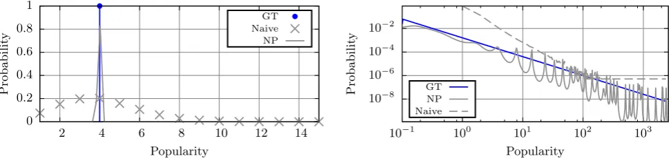
Figure 3: Mixing distribution obtained via the non-parametric methods for the #delta (left) and #prt(right) traces
be the proportion of documents with j requests, 1≤j≤J. Using (1), the log-likelihood`(g;µ) of the popularity distri-butiongfor the observationsµ= (µj)j≥1 reads as
`(g;µ) =
J
X
j=1
µjlogP[N=j|N >0]
=
J
X
j=1
µjlogEg
e−λλj j!
−logEg
h
1−e−λi.
We remark that in this setting, the catalog sizeKis decou-pled from the popularity distribution. Thus, we can first obtain an estimator ˆgof the mixing distributiong, and then approximateKby
ˆ
Kml= K0 Eˆg[1−e−λ]
(2)
which is asymptotically close to the ML estimator.
We now proceed with the detailed form of the likelihood function for theparametric and non-parametricestimation procedures. In both approaches, we numerically solve the problems with a generic non-linear optimization solver in MATLAB based on an interior point algorithm. Our code is freely available online.1 We discuss the use of specialized
algorithms in Section 7.
5.2.1
Parametric Estimation
In this setting, we determine the mixing distribution g
within a parametric family of density functions. The choice of that parametric family relies on an a-priori knowledge. The computation of the ML estimator obviously depends on this choice, and due to space restriction, we here limit ourselves to the two-parameter Pareto family with densities
g(x) =αxαm/xα+1 forx > xm, withα, xm the shape and
scale parameters, respectively. The log-likelihood function
`=`(α, xm;µ) then reads
`=
J
X
j=1
µjlog
Γ(j−α, xm)
j! −log (αx
α
m−Γ(−α, xm)).
5.2.2
Non-Parametric Family
In the absence of a-priori knowledge about the distribution
g, the non-parametric (NP) approach provides a method to obtain an estimator. In this setting, we determine a discrete distributiongof the formP[λ=xi] =θifor 1< i < I. The
1
Code :http://www.olmos.cl/code/mixed_poisson.tgz
log-likelihood correspondingly reads
`(θ;µ) =
J
X
j=1
µjlog I
X
i=1
θi
e−xixj
i
j! −log
I
X
i=1
θi(1−e
−xi).
5.3
Hit Ratio Analysis
As detailed in the Appendix 8, the IRM-M model proves to be tractable for evaluating the performance of an LRU cache. In particular, the so-called “Che approximation” is easily adapted to the IRM-M case; furthermore, we are able to derive formulas for the transient analysis of the hit ratio, when starting from an empty cache.
6.
NUMERICAL EVALUATION
The accuracy of the parameter estimation can be evalu-ated at three different levels, as expressed by the following questions: (1) Is the estimated popularity density close to the actual popularity density? (2)Is the request flow pre-dicted by the model statistically similar to the actual request flow? (3)Is the performance indicator of the fitted model, e.g., the hit ratio, accurately predicted?
Throughout this section, we assess the precision of a curve estimate by computing the so-calledmean absolute percent-age error (MAPE). More precisely, the MAPE between a reference sequence of points (xi)1≤i≤N and an estimate
se-quence (yi)1≤i≤N is defined by
MAPE(X, Y) = 1
N
N
X
i=1
|yi−xi|
|xi|
.
6.1
Estimation of popularity distribution
First, we start with the most general question, that is, the estimation of the mixing distribution. Such an inverse problem is known to be ill-posed.
For the NP estimation, we obtain an estimate ˆgnp of the
popularity density by applying the NP method, using a support with 0.01 as lower bound, exponentially increas-ing spacincreas-ings and an upper bound slightly larger than the maximum of observed requests (e.g., 2 400 for#prt and 16 for#delta). The naive fitting corresponds to the empirical measure of the request counts, that is, the mixture of Dirac measures 1
K0
PK0
k=1δnk(.).
10−1
100 101 102 103 104
100 101 102 103 104 105 106 107
F
requ
e
n
cy
Rank
GT Zipf
Figure 4: Rank frequency distribution for the #prttrace
valueλ = 4. In the #prt case, the estimated distribution is irregular, tending to accumulate mass at certain points (see Section 7.2 for possible regularization solutions). This concentration is no surprise, since in the non-censored case the ML estimator is discrete probability distribution [15]. The peaks, nevertheless, capture the power law trend, as reflected by the good estimation quality of the mixture dis-tribution. In contrast, the naive method fails at correctly estimating both the trend of distribution body and its tail.
Using Equation (2), we also calculate the catalog size, giving ˆK ≈ 11 600 000 (resp. 105 278) for the#prt (resp. #delta) case. This represents a relative error of 11.6% and 5.2%, respectively. Following Equation (2), it shows that es-timating the probability that a document receives no request for the duration of the trace, based on the very same trace, is a difficult task. As a consequence, this error is not negli-gible. It is, however, smaller, and even more significantly in the#prt case, than the relative error of the naive method (recall that ˆKnv=K
0= 1 900 000 and ˆKnv= 92 046 for the
#prtand#deltatraces, respectively).
When some a priori knowledge about the distribution shape is available, the estimates can be improved via the paramet-ric approach. In the#prtcase, the resulting Pareto fit gives the estimates ˆα= 1.597 and ˆxm= 0.099 that are very close
to the original parametersα= 1.6 andxm= 0.1. We
com-pare these results to that of the “log-log” approach, which consists in estimating the tail index by fitting a least square approximation to the log-log rank-frequency plot, as shown in Figure 4. The rank frequency plot roughly decays as 1/α. Using the first 20 000 objects to compute the regression, the estimation gives 1.704, which is worse than the ML estimate.
6.2
Request flow estimation
In this section, we specify the discussion by estimating the zero-censored request count distribution (or mixture distri-bution in statistical terms)P[N=j|N >0],j≥1.
For the naive approach, we generate 50 000 IRM traces using the estimated parameters. We then calculate the av-erage empirical distribution of the request per document. The number of generated traces ensures a coefficient of vari-ation lower that 10−4 for all points of the distribution. As
regards the ML approach, using the ˆgnpdensity, we compute
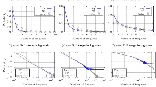
the associated zero-censored request distribution using (1). In Figure 5, we show the resulting zero-censored request distribution estimated by each method. For comparison, we include the real mixture distribution for the#prt dataset, which can be calculated explicitly. For the #yt and #vod
datasets, we show instead the observed request distribution. Two issues are raised by the naive approach, that are not present in the maximum likelihood estimation:
– first, at the head of the distribution, where most of the mass is concentrated, large estimation errors are produced by the naive approach. Such errors produce a mass shift to-wards the tail of the distribution. On the contrary, the NP estimation matches perfectly the head of the distribution; – second, the naive method over-fits the tail of the distribu-tion. We observe in Figure 5d that the naive estimate shows a “horizontal branch” at the tail, and differs significantly from the ground-truth that is approximately a straight “di-agonal” line. This horizontal branch is in fact a few isolated masses, though they look as a line on the figure. The naive estimation therefore concentrates the mass of the ground-truth distribution on a few points. On the other side, the ML estimation correctly estimates the trend of the distri-bution at all scales, though noise inaccuracies appear at the tail. This is quantified by the MAPE of 1.67 for the ML esti-mation, whereas the naive method leads to a MAPE of 668, for the full range distribution. As regards the#ytand#vod cases in Figures 5e and 5f, we similarly observe the same horizontal branch at the tail for the naive distribution. In the absence of available ground-truth, we do not compute the MAPE, but the similarity of behavior hints that the ML method also performs better on these traces.
6.3
Hit Ratio Estimation
We finally compare the hit ratios predicted by the IRM-M model with popularity distributions fitted using the naive and the ML methods, both for the#prtand#yttraces.
Figure 6 shows the obtained hit ratio curve in each case. The ground-truth curves are obtained by simulation of a LRU cache fed by the shuffled traces. The Naive (resp. NP) curves are obtained when using Formula (6) (resp. (9)) with the parameters obtained by the naive (resp. NP) method. Finally, the Zipf curve, for the #prt trace, corresponds to the hit ratio prediction when using the “log-log” parametric fitting method detailed in Section 6.1.
(a)#prt: First ten points
0 0.2 0.4 0.6 0.8 1
1 2 3 4 5 6 7 8 9 10
Pro
b
a
b
ili
ty
Number of Requests
GT NP Naive
(b)#yt: First ten points
0 0.2 0.4 0.6
1 2 3 4 5 6 7 8 9 10
Number of Requests
Emp NP Naive
(c)#vod: First ten points
0 0.1 0.2 0.3
1 2 3 4 5 6 7 8 9 10
Number of Requests
Emp NP Naive
(d)#prt: Full range in log scale
10−10 10−8
10−6 10−4 10−2
100 101 102 103
Pro
b
a
b
ili
ty
Number of Requests
GT NP Naive
(e)#yt: Full range in log scale
100 101 102 103 104 105 Number of Requests
Emp NP Naive
(f)#vod: Full range in log scale
100 101 102 103
Number of Requests
Emp NP Naive
Figure 5: Censored mixture distribution estimations obtained with the non-parametric method
0 0.2 0.4 0.6 0.8 1
0 0.2 0.4 0.6 0.8 1
H
it
Ra
ti
o
Relative Cache Size #yt: GT
#prt: GT
Naive Naive
NP
NP Zipf
Figure 6: Hit ratio for #ytand #prtdatasets. The cache size is normalized with respect to that of the ground-truth in the #prtcase and with respect toKˆml in the #ytcase.
leads to a significant error in the hit ratio estimation.
7.
DISCUSSION AND CONCLUSION
7.1
Other Applications and Extensions
Since our methodology requires only the statistics about the number of requests per document, the presented estima-tion method for content popularity can be readily applied in use-cases other than caching performance. For example, the
estimations can be used for dimensioning the bandwidth in the access network for VoD or TV multicast services or even predicting the demand for content in marketing studies.
Additionally, the wide applicability of the ML estimators makes our method a viable option for other traffic models. In particular, our framework can be extended to to renewal [6, 1] and cluster processes [17, 21]. In these cases new chal-lenges arises, due the reformulation of the ML method. For example, the randomized parameter in other traffic models is not univariate, but multivariate [17] or even an stochastic process [6]. Another factor to consider is time censure, due the greater impact of the time variable in stochastic models other than IRM-M.
7.2
Maximization techniques
The main current limitation of our maximization approach is that the estimated mixing density exhibits a lot of peaks, which is consistent with the results of Lindsay [15]. This might be a problem when one aims at understanding the nature of the popularity distribution.
A possible solution to enforce smoothness in the mix-ing density estimation is to introduce a penalization for the irregularities. Classical candidates for such a penal-ization are the L2-penalization or a logarithmic penaliza-tionR(θ) =PI
i=1(θi+1−θi)(logθi+1−logθi)/(xi+1−xi).
Another possibility is to exploit the fact that the peaks conserve the overall trend of the distribution. We thus ex-tract the peak locations. A second ML optimization is then performed using these peak locations as the new support. Though non-standard, this gives satisfactory results for the #prtdataset (not shown here due to lack of space).
7.3
Summary of results
In this paper, we have presented and solved the inverse problem that consists in estimating from a trace the popular-ity parameters for a performance model. A key point in our approach is that we consider the probability that a document receives a given number of requests, rather than the proba-bility that a request is directed to a given document. This representation is consistent with recently developed caching models [17, 21, 6]. Moreover, it allows us to avoid the fit-ting of a rank-frequency plot, which is in essence an order statistic and exhibits over-fitting. Our second contribution on the modeling aspects is that we consider popularities as random variables, rather than parameters, leading to a mix-ture model tractable via ML methods. We have illustrated our method in the case of cache performance evaluation but our framework is applicable and extensible to other settings. The inverse problem stems from the random nature of the requests countNfor a given document. In particular, a traf-fic trace contains a single sample of these requests counts. The accuracy of any method that aims at fitting indepen-dently the popularity of each document is therefore limited by the inherent variability of the random variableN. The importance of using a sound methodology correspondingly increases when the variability of the request counts is large, which is typically the case whenN is small.
Determining the parameters of the model allows one to use the performance for diverse objectives, including the dimen-sioning of operational networks or the design of new mecha-nisms. More importantly, in contrast with simulation-based analysis, it enables one to more easily explorewhat-if sce-narios, by keeping some parameters at their current value and modifying others to reflect future or possible changes.
8.
APPENDIX
We here detail the derivation of hit ratio formulas for the IRM-M model.
8.1
IRM Model
For comprehension purposes, we first briefly review the “Che approximation” method for the hit ratio estimation in the IRM model (additional details can be found in [7]). Given popularitiesλ1, λ2, . . . , λK, letXk(t) denote the
num-ber of different documents, apart from thek-th, requested in a time window [0, t], that is,
Xk(t) =
K
X
i=1;i6=k
1{Ni[0, t]≥1}.
Let TCk = inf{t > 0 : X k
(t) ≥ C} be the exit time to levelCfor processXk;TCk represents the eviction time for
content k in a LRU cache of size C, given that it is not requested during this time period. Now, the core of the “Che approximation” consists in the two following steps:
1. allTk
Chave the same distribution, i.e.,∀k, TCk
d
=TC;
2. the random variableTCis well approximated by a
con-stanttC called the “characteristic time”. The timetC
is implicitly defined by the equation
K
X
k=1
E[1{Nk[0, tC]≥1}] = K
X
k=1
1−e−λktC =C. (3)
Intuitively,tC is the time when, on average,Cdifferent
ob-jects have been requested.
In the stationary case, the hit ratioHcan then be derived as follows. Using the PASTA property, the hit ratio of doc-umentkfor a cache of sizeC is equal to 1−eλktC, and by
averaging on all documents, it follows that
H ≈ 1
Λ
K
X
k=1
λk(1−e
−λktC). (4)
In the transient case, we simply assume that Tk C ≤ W
(the hit ratio does not increase with Tk
C when TCk > W).
By independence, it can be shown (see Proposition 3, [17]) that the average number of hits for the k-th document in a time window of sizeW, starting from an empty cache, is E
h(λk, TCk)
where the expectation carries onTCk and the
functionh(λ, t) is defined by
h(λ, t) = (λW−1)(1−e−λt) +λte−λt, t < W. (5) In consequence, setting Λ =PK
k=1λk, the transient hit ratio
H(W) is given by
H(W) = 1 ΛW
K
X
k=1
Ehh(λk, TCk)
i
.
Applying the “Che approximation”, we then obtain the fol-lowing formula for the hit ratioH=H(W):
H≈ 1
Λ
K
X
k=1
λk(1−e−λtC)+
1 ΛW
K
X
k=1
λktCe−λktC −C
!
. (6)
The second term of (6) vanishes as W → ∞, leading to equality (4) for the stationary hit ratio.
8.2
IRM-M Model
We now address the IRM-M case. We first show how to derive the hit ratio in this setting; we further prove formally the validity of the “Che approximation” in the case where
C=δK andKtends to infinity.
•Given the popularitiesλ1, λ2, . . . , λK, let us defineXk,
TCk as in the previous section, and let δ = C/K be the
proportion of stored documents. As the popularities are here an i.i.d. sample, and sinceXkandTk
Care independent
of λk, the previous quantities do not consequently depend
on the document indexk. In consequence, this validates the first step of the “Che approximation”.
For the second step, define the characteristic timetδ as
tδ=r
−1
(δ) with r(t) =Eh1−e−λti, (7) which is equivalent to dividing both sides of (3) byK. Fol-lowing the same steps as in the previous section, it is easy to derive the following hit ratio formulas:
H≈E
λ(1−e−λtδ)
E[λ] , (8)
H(W)≈E
λ(1−e−λtδ)
E[λ] + E
λtδe−λtδ
−δ
Equations (8) and (9) are the IRM-M analogs of (4) and (6).
• We show that the second step of the Che approxima-tion is asymptotically exact, that is, the random variable
TCcan be replaced by the associated characteristic timetδ.
Consider the case where the cache size scales with the cata-log size, that is,δ remains constant, andC andKgrow to infinity. Recall that the distribution ofTC is given by
P[TC> t] =P
" K
X
k=1
1{Nk[0, t]≥1}< C
#
fort≥0, which can be rewritten as
P[TδK> t] =P
"
1
K
K
X
k=1
1{Nk[0, t]≥1}< δ
#
. (10)
An application of the law of large numbers shows that
lim
K→∞
1
K
K
X
k=1
1{Nk[0, t]≥1}=r(t)
almost surely; using (10),TδKthus converges in probability
to the constanttδ, forδ∈[0, r(W)], withr(W) =E[K0]/K.
By the conditioning argument of Proposition 3 in [17], it can be shown that the expectation of the number of hits
HC=HδK satisfies the identity
E[HδK] =E[h(λ, TδK)] ;
applying then the bounded convergence theorem (Section 13.6, [22]) to the latter identity and dividing by the expected number of requestsE[λ] leads to formulas (8) and (9), as claimed.
9.
REFERENCES
[1] D. S. Berger, P. Gland, S. Singla, and F. Ciucu. Exact analysis of TTL cache networks.Performance
Evaluation, 2014.
[2] Y. Carlinet, T. D. Huynh, B. Kauffmann, F. Mathieu, L. Noirie, and S. Tixeuil. Four Months in
DailyMotion: Dissecting User Video Requests. In8th International Wireless Communications and Mobile Computing Conference (IWCMC). IEEE, 2012. [3] M. Cha, H. Kwak, P. Rodriguez, Y.-Y. Ahn, and
S. Moon. I tube, you tube, everybody tubes: Analyzing the world’s largest user generated content video system. In7th Conference on Internet
measurement (IMC). ACM, 2007.
[4] A. Clauset, C. R. Shalizi, and M. E. Newman. Power-law distributions in empirical data.SIAM Review, 2009.
[5] F. Comte and V. Genon-Catalot. Adaptive Laguerre density estimation for mixed Poisson models. Electronic Journal of Statistics, 2015.
[6] N. C. Fofack, P. Nain, G. Neglia, and D. Towsley. Analysis of TTL-based cache networks. In6th International Conference on Performance Evaluation Methodologies and Tools. IEEE, 2012.
[7] C. Fricker, P. Robert, and J. Roberts. A Versatile and Accurate Approximation for LRU Cache Performance. In24th International Teletraffic Congress (ITC). IEEE, 2012.
[8] C. Fricker, P. Robert, J. Roberts, and N. Sbihi. Impact of traffic mix on caching performance in a
content-centric network. InConference on Computer Communications. IEEE, 2012.
[9] P. Gill, M. Arlitt, Z. Li, and A. Mahanti. YouTube traffic characterization: A view from the edge. In7th Conference on Internet measurement). ACM, 2007. [10] W. Gong, Y. Liu, V. Misra, and D. Towsley. On the
tails of web file size distributions. InAnnual Allerton Conference on Communication Control and
Computing, 2001.
[11] F. Guillemin, B. Kauffmann, S. Moteau, and A. Simonian. Experimental analysis of caching efficiency for youtube traffic in an ISP network. In25th International Teletraffic Congress (ITC). IEEE, 2013. [12] L. Guo, E. Tan, S. Chen, Z. Xiao, and X. Zhang. The
stretched exponential distribution of internet media access patterns. In27th Symposium on Principles of distributed computing. ACM, 2008.
[13] C. Imbrenda, L. Muscariello, and D. Rossi. Analyzing Cacheable Traffic in ISP Access Networks for Micro CDN Applications via Content-centric Networking. In 1st International Conference on Information-Centric Networking, ICN ’14. ACM, 2014.
[14] D. Karlis. A General EM Approach for Maximum Likelihood Estimation in Mixed Poisson Regression Models.Statistical Modelling, 2001.
[15] B. G. Lindsay. Mixture Models: Theory, Geometry, and Applications.Institute for Mathematical Statistics: Hayward, CA, 1995.
[16] P. Loiseau, P. Gon¸calves, S. Girard, F. Forbes, and P. Vicat-Blanc Primet. Maximum Likelihood Estimation of the Flow Size Distribution Tail Index from Sampled Packet Data. InPerformance Evaluation Review. ACM SIGMETRICS, 2009. [17] F. Olmos, B. Kauffmann, A. Simonian, and
Y. Carlinet. Catalog dynamics: Impact of content publishing and perishing on the performance of a LRU cache. In26th International Teletraffic Congress (ITC). IEEE, 2014.
[18] B. N. Oreshkin, N. Regnard, and P. L’Ecuyer. Rate-based daily arrival process models with application to call centers. Technical report, 2014. [19] J. Roberts and N. Sbihi. Exploring the
memory-bandwidth tradeoff in an information-centric network. In25th International Teletraffic Congress (ITC). IEEE, 2013.
[20] F. Roueff and T. Rydn. Nonparametric estimation of mixing densities for discrete distributions.The Annals of Statistics, 2005.
[21] S. Traverso, M. Ahmed, M. Garetto, P. Giaccone, E. Leonardi, and S. Niccolini. Temporal locality in today’s content caching: Why it matters and how to model it.Computer Communication Review, 2013. [22] D. Williams.Probability with Martingales. Cambridge